The Price Determinants of the EU Allowance in the EU Emissions Trading Scheme

Abstract

The Kyoto Protocol came into effect in 1997 to curb greenhouse gas (GHG) emissions and to address the problem of climate change. The Protocol includes a market-based mechanism designed to offset GHG emissions, called the emissions trading scheme (ETS), allowing companies to “trade” their shortage or surplus allowance. This study examines the determinants of the EU allowance (EUA) price in Phase 3 of the EU ETS (2013–2017). First, the causality between the EUA price and other variables is determined using a Granger causality test. Second, the correlation between the EUA price and each variable is measured using a VECM estimation and an impulse response function. Finally, the relative effect of each variable on the EUA price is determined using a forecast error variance decomposition. The results show that the EUA price has a causal effect on the prices of electricity and natural gas. Second, all variables, except the minimum temperature, show a positive relationship with the EUA price. Furthermore, when unexpected shocks occur, the EUA price shows the highest response to its past price, followed by the electricity price. Third, the past EUA price has the most influence on the EUA price, followed by the coal price.

1. Introduction

The increase in man-made greenhouse gas (GHG) emissions has caused problems related to climate change. As a result, the international climate change community is striving to stabilize global GHG levels by restricting emissions.

In 1997, world leaders met in Kyoto, Japan and established the Kyoto Protocol, which helps countries meet emissions targets and encourages the private sector and developing countries to reduce their emissions. It includes three market-based mechanisms: emissions trading (ET), a clean development mechanism (CDM), and joint implementation (JI). The emissions trading scheme (ETS) is based on these market mechanisms.

The ETS works on the principle of “cap and trade”, which means a government can set a limit on GHG emissions for companies (a “cap”), and then allow them to “trade” these rights in the market [1]. Unlike existing regulations that enforce uniform standards on all companies, the ETS allows companies to choose the approach most favorable to their situation and then to buy and sell their carbon emissions allowances.

According to the International Carbon Action Partnership (ICAP), since the European Union (EU) was established in 2005, 21 systems have been put in place covering 28 jurisdictions. This means that economies using an ETS produce more than 50% of the global GDP and that a third of the world’s population are living in jurisdictions that are considering, preparing, or operating an ETS [2,3].

The European Union Emissions Trading Scheme (EU ETS) represents the EU’s climate change policy and is one of the most comprehensive schemes [2]. The first phase of the EU ETS began in 2005, and it is now in its third phase, with 31 countries participating [4]. In the global ETS market, the EU ETS has the largest volume and value (5121 Mt and EUR 30,760 million, respectively), representing 74% of the total global ETS value and share [5]. In addition, the EU is planning to activate a wider carbon trading market through international cooperation with Switzerland [2].

In an ETS, the emission allowance price (or “carbon price”) is important, because if it is set too low, it cannot offset the climate damage and may also be overused [6]. Companies may choose to simply buy what they need rather than reducing their emissions. A low price would also not encourage companies to replace high carbon-emission fuels, such as coal and oil, with natural gas or low-emission fuel. Therefore, setting an effective carbon price is a critical part of maintaining an ETS system.

This requires that we understand the factors that determine the price. Therefore, this study focuses on the EU ETS and examines the determinants of the European Union allowance (EUA) price using various variables and methods. As such, this study has three primary goals. First, we use a Granger causality test to find the causal links between the EUA price and other variables. Second, we use a vector error correction model (VECM) estimation and an impulse response function to measure the correlation between the EUA price and each variable. Third, we use a forecast error variance decomposition to compare the relative influence of the variables on the EUA price. To do so, we employ variables used in previous studies, in addition to several new variables; which have been added because their exclusion was identified as a limitation in previous studies [7,8,9].

The EUA futures price is used as the price variable. The variables included here that are based on those of previous studies are related to energy (oil, coal, electricity, natural gas), economics (industrial production, economic sentiment), temperature (precipitation), and certified emission reduction (CER). Moreover, the following three variables have been added: bank lending rate, maximum temperature, and minimum temperature.

The methodology for our empirical test is as follows. First, we check the correct lag order using the Schwarz Bayesian information criterion (SIC). Second, we check the stability of the time series data using unit-root tests such as the augmented Dickey–Fuller (ADF) and Phillips–Perron (PP) tests. Third, we check for cointegration between the variables using the Johansen cointegration test. Fourth, the causal factors of the EUA price are determined using the Granger causality test. Fifth, we measure the correlation between the EUA price and each variable using a VECM estimation and an impulse response function. Finally, we compare the relative effect of each variable on the EUA price using a forecast error variance decomposition.

The research period is set as January 2013–December 2017 because this coincides with the third phase of the EU ETS. We use the statistical analysis tool, EViews, and all data are monthly.

The remainder of the paper is organized as follows. Section 2 presents a literature review and compares this study to past works. Section 3 provides a theoretical background and explains the carbon price mechanism. Section 4 describes our methodology and data, as well as the results of the empirical tests. Section 5 presents the conclusions and implications of the study.

2. Literature Review

Numerous studies have identified the main determinants of the emission allowance price as energy prices, macroeconomics, climate, and CERs.

First, energy prices can be divided into the prices of oil, coal, and gas. Since these sources of “electricity” are also based on energy generation, it is reasonable to include the electricity price among the energy price variables. Based on an economic analysis, Christiansen et al. [10] analyze a number of key factors that influence the price of the emissions allowance in the EU ETS in the period 2005–2007, finding that fuel prices affect the allowance price. Bataller et al. [11] and Alberola et al. [12] analyze the relationship between the allowance price and the energy market, showing that energy sources are the most important determinants of allowance price levels. Bunn and Fezzi [13] analyze the mutual relationships between electricity, natural gas, and the allowance price in the daily spot markets in the United Kingdom, showing that the allowance price and natural gas jointly influence the equilibrium price of electricity. Tan and Wang [14] focus on the quantile-based dependence and influence path between the EUA and its drivers during the three EU ETS phases. They find that energy variables such as the prices of Brent crude oil, natural gas, and coal have significant impacts on the carbon price (EUA futures). In comparison with phase 1, they find more asymmetric dependences of the impact of energy in phases 2 and 3, and that the EUA–energy dependence is stronger than it has been in the past. Hong et al. [15] employ various statistical methods to predict European carbon price movements, and find that Brent crude futures (oil) and natural gas are statistically significant in terms of forecasting CO₂ price movements, having a positive and a negative relationship with it, respectively.

Second, addressing macroeconomic variables, Chevallier [16] questions how economic shocks may affect the carbon markets. He proves that the carbon price tends to respond negatively to an exogenous shock that reduces the global economic indicators by one standard deviation and establishes that they have a relationship with the allowance price. Oberndorfer [17] finds that the EUA price and the stock returns of the most important European electricity corporations are positively related. The relationship is particularly strong for the period of the EUA market shock in early 2006, and is different for the countries where the electricity corporations are located. Lin and Kim [18] analyze the causes of CO₂ prices and the stock prices of steel corporations using a time-series model. They prove that the stock prices affect the allowance price, but not vice versa. Moreno and Silva [19] investigate the EUA price using stock market returns of Spanish polluting sectors. They find a statistically positive and negative impact on these stock market returns during phase 2 and phase 3, respectively. They also find that the effects and responses of EUA prices differ by sector. Koch et al. [20] examine why the EUA price drops, showing that its dynamics cannot be explained solely by marginal abatement cost theory and that the economic sentiment indicator is a particularly useful economic state variable for explaining price movements.

Third, Christiansen et al., Mansanet-Bataller et al. and Alberola et al. [10,11,12] analyze which climate factors influence the allowance price. Alberola et al. [12] find that when the weather is extreme, power generators have to produce more or less than forecast, which contributes to a respective increase or decrease in the allowance demand and CO₂ prices. Moreover, they explain that unanticipated temperature changes seem to matter more than the temperatures themselves. Benz [21] also shows that unexpected changes in the weather lead the allowance price level.

Fourth, a CER is one of the variables that affect the allowance price. CERs and emission reduction units (ERUs) are issued by CDM projects and JI projects. After they are registered with the UN, they can be linked with the EU ETS and recognized as an emission allowance. Barrieu and Fehr [22] argue that EUAs and CERs are closely linked. However, a CER carries more risk than an EUA, which means the price of a CER is less than that of an EUA. If CDM projects are activated, then the allowance supply will increase, which will influence the EUA price level. In the market, EUAs, CERs, and AAUs are traded equally, which means companies will buy the relatively cheaper CER, which affects the allowance price. Chevallier [16] finds that during an economic downturn, CER futures prices tend to react more significantly than EUA spot and futures prices do. Koch et al. [20] argue that the effect of CERs on EUA price dynamics seems limited, but that a potential increase in the number of issued CERs will affect the allowance price.

Since much attention has been given to factors affecting the allowance price, studies have applied these variables to determine the efficiency of the market or have combined them to analyze the price determinants. Hintermann [23] uses climate and energy price variables to investigate the efficiency of the market, finding that the marginal abatement cost (MAC) influences the allowance price if the market is efficient. However, in the first phase the MAC had no influence on the allowance price, which means the market was not efficient. Other studies have combined various factors to determine the relative significance of each of the variables in affecting the allowance price. There are four main studies in this line of research [24,25,26,27].

In contrast, Lee and Pak, Cho, and Hong et al. [25,26,27] use EUA futures prices instead of the spot prices. Lee and Pak [25] use a VECM analysis to identify the determinants of the allowance price in the first and second phases. According to their research, the oil price has a positive relationship with the allowance price. If the economy is in a growth period, the demand for oil increases. As a result, CO₂ emissions increase. Thus, both the oil price and the allowance price increase. They also show that the coal and electricity prices have negative relationships with the allowance price. They argue that the CER variable has the most significant relationship with the allowance price, and that the EUA futures and CER prices move in the same direction. Therefore, they conclude that the CER variable is the most significant.

In particular, this study builds on the works of Lee and Pak [25] and Cho [26]. We use allowance futures price data and regression tests to explain the determinants of the allowance price. This study adds to the literature by including variables for extreme temperatures (rather than average temperatures) and the euro area bank lending rate. We focus on the third period of the EU ETS (2013–2020). Using recent data is important because, as shown in Bu and Jeong [27], the relevance of the variables changes over time. In addition, as shown in Hintermann [23], the EU emissions system was not effective in the first phase and had over-allocation problems because the marginal abatement cost did not work properly in the market. Thus, the third-phase data are the most current and accurate.

3. Theoretical Background and Carbon Price Mechanism

3.1. Theoretical Background

3.1.1. Understanding the Emissions Trading System

The effects of climate change are exacerbated by GHG emissions, which need to be addressed.

Accordingly, many studies have investigated methods for reducing emissions. This led to the 1992 United Nations Framework Convention on Climate Change agreement which did not, however, discuss how to reduce GHG levels. Therefore, in 1997, world leaders met again in Kyoto, Japan, and established the Kyoto Protocol which included three market-based mechanisms: emissions trading (ET), CDM, and JI.

After the Kyoto Protocol was activated in 2005, the market-based mechanisms led to some success, but there are also limitations. Developed countries are dissatisfied with imposing excessive reduction obligations on themselves only. In addition, after the first phase (2008–2012), there was little confidence that it would continue. Thus, in 2015, global leaders met once again to create the Paris Agreement. This is a bottom-up mechanism, in which each country chooses its own emission reduction goal (nationally determined contribution) and pursues it autonomously, allowing developing countries to take responsibility for their emissions. In addition, the agreement does not include a legal restraint and there is no end date. This encourages more countries to participate and is more sustainable than the Kyoto Protocol. However, it is still under debate, and it is unclear whether it will be activated before 2020 [28].

The ETS is based on the Kyoto Protocol market mechanism. It works on the “cap and trade” principle where governments impose a limit (cap) on total emissions in one or more sectors of the economy. Companies in these sectors need to hold one permit for every tonne of emissions [1]. Each year, some free allowances are allocated, while the rest are sold, mostly through auctions. At the end of each year, participants must return one allowance for every tonne of CO₂ emitted. If a participant has insufficient allowances, it must either reduce emissions or buy additional allowances in the market. Participants can acquire allowances at auctions, or by trading [4].

Governments can tailor their ETS to suit local conditions, such that each system presents its own unique approach. Currently, systems operate at a range of administrative levels, from megacities (e.g., Tokyo) to US states and Canadian provinces, as well as at the supranational level (e.g., the EU). An ETS is based on an understanding that the cost of reducing emissions varies between countries. Therefore, they do not force parties to use a single system or hinder economic efficiency, and tend to encourage emission reductions. As a result, an ETS decreases GHGs and encourages emission reduction technology development.

3.1.2. Current Status of the Global Emissions Trading System

The volumes and values of the major global carbon markets are diverse [5]. In 2017, the European market had the largest trading volume and value, at 5121 Mt (72.76%) and EUR 30,760 million (74.43%), respectively. North America has the second largest values of 952 Mt (13.52%) and EUR 9328 million (22.57%), followed by New Zealand, China, and South Korea.

Not only do the trading volumes and values vary by country, but the systems also work differently. Some countries have national-level ETSs (the EU, South Korea, New Zealand), whereas others (North America and China) organize at the local level. In North America, California linked its system to that of Quebec and later Ontario. China first activated local ETSs, and at the end of 2017, launched its much-anticipated national ETS (activation is imminent). The purpose of local ETSs is to select the most suitable national system. After establishing the Shenzhen ETS in June 2013 China established seven additional local ETSs, which all have different rules and coverage.

Diverse ETS systems are used in various countries [2,29]. First, there are some differences in terms of auction use. The EU and North American (California) ETSs use auctioning and free allowances. Other countries only use free allowances. While auctioning is not a perfect method for distributing allowances, it is an efficient way to obtain permits for those who value them most. Auctions generate public revenue and provide an incentive for early action against climate change. Furthermore, auctioning is also fair, ensuring that regulated companies pay for their emissions. Currently, the EU is using at least 50% of its auctioning revenue for climate actions. Thus, it funds one of the world’s largest programs for low-carbon innovation, the NER 300. Most of the Californian auction revenue goes to the GHG reduction fund, of which at least 25% is used to benefit disadvantaged communities [30].

Second, there are differences in terms of offsets, banking, and borrowing. Currently, only the EU is using the international offset, which allows the use of JI and CDM. By helping other countries reduce their GHGs, they earn ERUs and CERs that can be exchanged for EUAs. Banking means companies can save their emission surplus and use it later, whereas borrowing means they can borrow their future allowance and use it today. Countries tend to allow banking, but not borrowing, because they do not believe the latter will reduce emissions. South Korea allows borrowing, but limits it to 10% of the required allowance.

Third, is the carbon price difference. If the price is too low, companies might feel less of an economic burden, reducing their incentive to decrease emissions or develop low emission techniques as it is cheaper to buy allowances and continue to use high emission material. Currently the cheapest price is in the Chinese market. The most expensive Chinese allowance is the Beijing pilot (USD 7.5), and the cheapest is that in Tianjin (USD 1.36), more than 15 times cheaper than the most expensive option in South Korea (USD 20.66). Therefore, China’s carbon price needs to increase if its national system is to be successful [29].

In the next section, we examine ETS systems in general and the EU ETS system in particular.

3.1.3. The Development Background of the EU Emissions Trading System

After the Kyoto commitments, in March 2000, the European Commission presented a green paper on “GHG emissions trade within the European union” with some initial ideas for the design of the EU ETS. This led to the adoption of the EU ETS directive in 2003 and its introduction in 2005. Through Phase 1 (2005–2007) and Phase 2 (2008–2012), it is now in Phase 3 (2013–2020), which makes it the most developed, mature carbon market with the biggest trade value and volume in the current worldwide ETS system.

The key features of the third phase are documented in the 2018 ICAP Report [31]. First; they make the EU ETS stricter and, thereby, increase the carbon price. This is because even though more countries are joining the EU ETS and its GHG coverage is increasing, it is reducing the cap and applying stricter requirements on CERs and ERUs. Thus, it seems reasonable to assume their purpose is to increase their carbon price.

Second, the allocation method is changing from free allocation to auctioning. Auctioning offers an effective way to obtain permits and increases public revenue. The EU ETS is using more than 50% of the revenue generated from auctioning of allowances to combat climate change in the EU and developing countries.

In particular, electricity production uses auctioning only, and the industry sector is reducing its use of free allowances and increasing the use of auctioning. However, this does not mean that they are not using free allowances for their allocations. Any sector that faces a significant risk of carbon leakage owing to the price of CO₂ will continue to receive up to 100% free allocations [4].

Finally, the free allocation method is changing from grandparenting to benchmarking. There are three methods for free allocation: grandparenting, benchmarking, and updating. The EU ETS used grandparenting in Phases 1 and 2. “Grandparenting means the companies receive a free allowance based on their historical emission from a specified period” [31]. For example, if company A emits 30 Mt CO₂ in 2005 and sets this as its standard, then its subsequent performance is based on this 2005 emission data. In addition, if they do much better than 2005, then the free allowance is increased. This free allocation method is relatively simple, with moderate data requirements. However, the disadvantage of this method is that it may reduce the need to trade in earlier years. In addition, the reduction amount between small companies, which should reduce their emissions by a small amount, and big companies, which should reduce their emissions by a large amount, shows a large gap. Therefore, many big companies feel the system is unfair.

Benchmarking means “the companies receive a free allowance depending on a set of performance standards, based on the emission intensity of a product across a sector” [31]. For instance, if company A emits 10 Mt CO₂, and reduces this to 9 Mt CO₂ in 2016, and then in 2017 reduces it further to 8 Mt CO₂, its decrease (in percentage terms) is more in 2017 than in 2016. Thus, it will receive a relatively higher free allowance in 2017. Benchmarking needs more high-quality data than grandparenting does, but it means that big and small companies obtain free allowances based on their performance, rather than on their historical emissions, making it a fairer system [31]. In addition, it encourages all companies to invest in clean technology, thus reducing GHG emissions effectively.

We now briefly discuss the transaction trends in the trading of various products. The 2018 ICAP report shows the 2014–2016 transaction volume (Mt CO₂) and value (EUR million) for the EU ETS [32]. Based on the report, two facts are evident. While EU futures are the most traded products, accounting for more than 70% of all trades between 2014 and 2016, other products seem to be decreasing in terms of their value and volume (especially CERs). Only EUA auctions increased in volume and value, proving that changing from free allocation to auctioning led to this increase.

3.2. Carbon Price Mechanism

3.2.1. Importance of the Carbon Price

Pollution is costly as it leads to drought and floods, as well as extreme weather conditions. Even though the damage from the disposal of emissions may be USD 30 or USD 40 per tonne at present, people cannot simply stop driving, heating, or using electricity [6].

Carbon pricing offers a solution as it is the most cost-efficient way to reduce emissions by giving polluters an economic motivation to do so. It not only reduces emissions, but also generates revenue, creates jobs, and helps the community.

For the carbon price to work it should be relatively high, otherwise it cannot offset the climate damage and it might still be cheaper to purchase an allowance and continue using high-emission fuels instead of low-emission fuels.

However, an exorbitant price may reduce the motivation to use the system. For example, poorer countries may heavily discount the future, and not actively participate in carbon pricing because they are more concerned about their present economic circumstances. Second, developed countries may feel that developing countries are “free riding”, which is defined as “doing little and expecting to benefit sufficiently from other countries mitigation” [6]. For example, the United States did not participate in the Kyoto Protocol because it felt that China had no incentive to reduce their high emission levels. Third, countries that export oil or coal may want a low carbon price, because a higher price suppresses demand and reduces profit.

This makes it difficult to set a high carbon price, creating challenges for overall environmental policies. In the next section, we discuss the current cap and trade mechanism in further detail.

3.2.2. Cap and Trade Benefits

ETSs currently allow governments to cap emission allowances, and companies can trade for a surplus or purchase allowances on an auction if they have a shortage. Each country can tailor its ETS according to its economic situation and unique background. This not only reduces GHG emissions, but also generates revenue through auctions. Therefore, many countries are joining the ETS system because of its flexibility.

According to the EU Commission [4], there are four main benefits of using this system. First, there is certainty over quantity. Setting a system cap ensures the emissions objective is more likely to succeed.

Second, it is cost effective because firms face the same carbon price. Companies can only sell allowances if they reduce their emissions.

Third, the system generates revenue from auctioning, which can be used to develop communities or invest in environmental projects.

Finally, the system can be linked to other ETSs to obtain additional benefits. The EU ETS is already linked to those of many other countries, which means companies do not need to buy international units to meet commitments in other countries.

It also has several limitations, which are discussed in the next subsection.

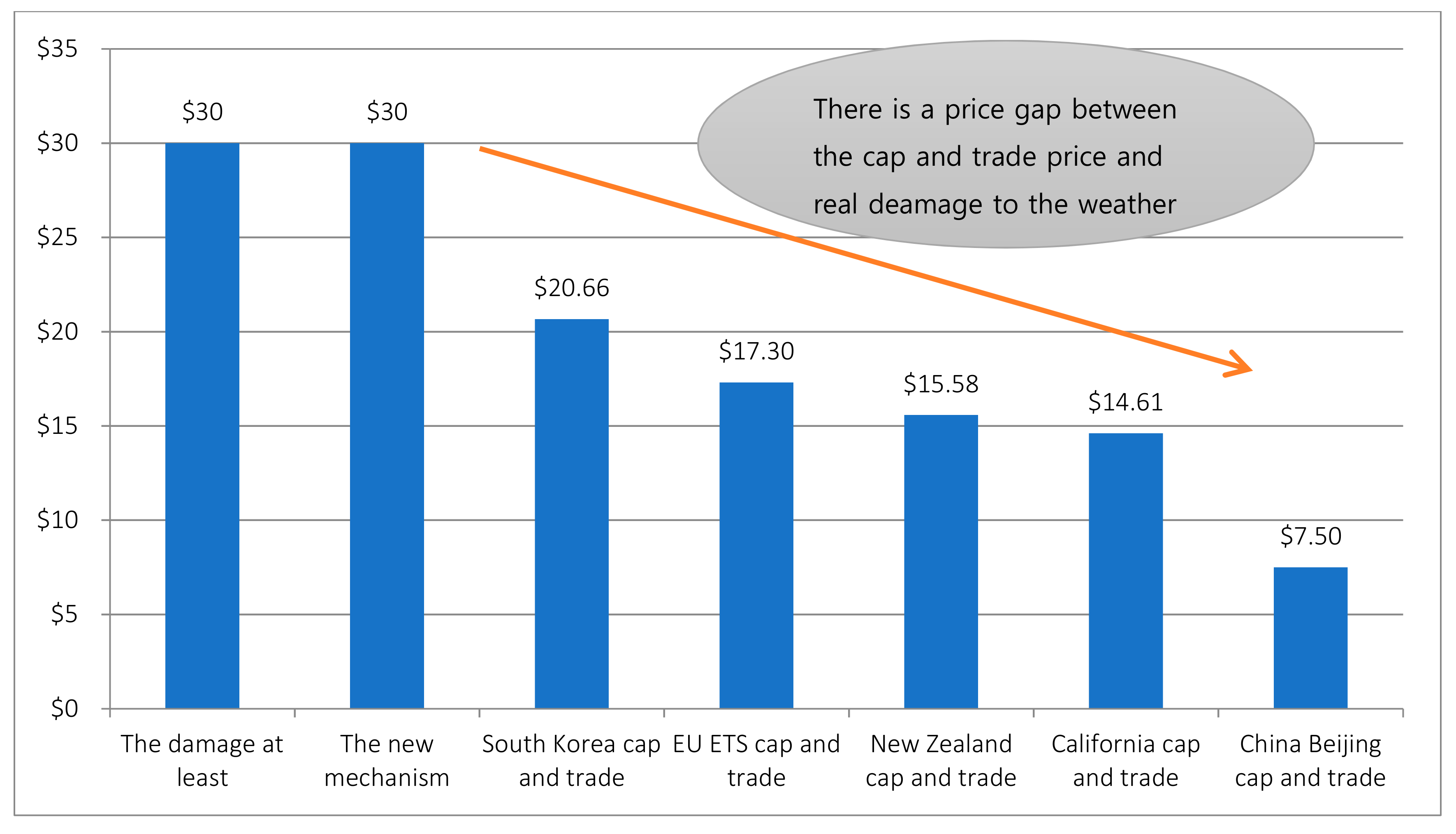
3.2.3. Global Carbon Pricing Mechanism

Some researchers assert that the current mechanism has limitations in controlling climate change, believing that a new global carbon pricing mechanism will be necessary once the Paris Agreement is implemented.

Cramton et al. [6] assert that there are two limitations to the current mechanism. First, it requires that all emitters in all countries trade permits in one unified market. The EU ETS has such a policy, but it only covers half of all emissions, and only exists because the EU has a single government.

Second, the current carbon price level is too low to offset the damage of GHG emissions. The cost of disposing of one tonne of GHG is at least USD 30 at present [6]. However, the current carbon price level is much lower (USD 17.3 in the EU ETS), as shown in Figure 1.

Cramton et al. [6] state that the global carbon price mechanism is an agreement between countries responsible for most of the world’s GHG emissions to price their own fossil-fuel emissions at least as high as the agreed-on global price.

It means that a future mechanism should include all countries and consider the world as a whole, rather than just the local externalities that a country causes. In addition, setting the lowest “conditional price” (according to GHG emissions) has caused damage to the overall climate. For example, if one country’s carbon price is USD 6 and the local externalities are USD 5, it benefits by USD 1. However, some GHGs, such as CO₂, do not cause local externalities, but instead have a global effect. Therefore, if the world externalities are USD 25, the country can benefit by USD 1, but harm the world climate by USD 24.

Setting the price according to global GHG damage seems rational, but whether it can be used in practice remains to be seen, because it may be too expensive for developing countries, hampering their industrial development. Cramton et al. [6] assert the importance of a global carbon pricing mechanism sharing a common commitment and offering a reciprocal deal that poorer countries can use and wealthier countries can trust.

Hence the emphasis on the role of green climate funds, which reduce the differentiation in responsibilities between richer and poorer countries. The climate fund formula is defined as ${\mathrm{G}}_{\mathrm{i}}=\mathrm{g}\times {\mathrm{X}}_{\mathrm{i}}\times \mathrm{P},$where g is a generosity parameter, ${\mathrm{X}}_{\mathrm{i}}$ is the excess emissions of country i, and P is the global price. Funds are transferred from rich to poor countries, which has positive effects for both. Previously, poorer countries set low carbon prices to protect their development. However, funds are transferred to poor countries first, which means they can pledge a higher carbon price P. In addition, it benefits the rich countries because the common carbon price eliminates free riding and lack of transparency. Furthermore, richer countries can collect more revenue than they pay in abatement. Cramton et al. [6] state that if one tonne of GHG costs USD 30 and GHGs are reduced from 1 billion tonnes to 0.8 billion tonnes, then 0.8 $\times$ USD 30 = USD 24 billion will be collected in revenue. However, the formula shows that C = P $\times \frac{\mathrm{A}}{2}$. Thus, the cost of abatement is USD 30 (price of carbon)$\times$ 0.2 ÷ 2 (the reduction in the amount of carbon ÷ 2) = USD 3 billion (eight times less than the revenue collected).

They [6] also compare the global carbon pricing mechanism with the cap and trade mechanism using China in 1999 as an example. The results show that the cost to China would have been more than 12 times greater under the cap and trade mechanism than under the global carbon pricing mechanism.

Finally, the most important part of the global carbon pricing mechanism is the common commitment and reciprocal trust.

4. Empirical Analysis

4.1. Data and Model

4.1.1. Variables and Data

This study uses several variables (see

Table 1. Variables and statistical data.

Variable Classification	Variable	Variable Description	Source of Data
Price	EUA (Allowance Price)	EUA Futures Price	www.investing.com
Energy	COAL (Coal Price)	Australian Thermal Coal Price	www.indexmundi.com
	BRENT (Oil Price)	Brent Futures Index	www.theice.com
	GAS (Natural Gas Price)	European Nature Gas Future Index
	ELEC (Electricity Price)	UK Power Future Index
Economic	IPI (Industrial Production)	European Industrial Production Index	www.ecb.europa.eu
	ESI (Economic Sentiment)	European Economic Sentiment Index	www.ec.europa.ev/eurostat
	Lending (Bank Lending)	Euro area Bank Lending Index	www.tradingeconomics.com
Temperature (new)	TEMPMAX (Temperature Maximum)	European Average Temperature Maximum Index	www.worldweatheronline.com
	TEMPMIN (Temperature Minimum)	European Average Temperature Minimum Index
	PRE (Precipitation)	European Average Precipitation Index
Related index	CER (Certified Emission Reduction)	CER Futures Price	www.marketwatch.com

), including those of previous studies and three new variables. Many studies have examined the determinants of the allowance price in the first two phases of the EU ETS. However, little is known about Phase 3. Therefore, we focus on Phase 3 (2013–2017), using monthly data for 12 variables. For the empirical analysis, we use EViews (EViews is a statistical package for Windows, used mainly for time-series-oriented econometric data) version 10. The aim of this study is to find the price determinants of EU allowances.

We use the EUA futures price for the price variable. There are several reasons for this choice. First, more people are trading in EUA futures than in the spot market. In 2016, the overall EU futures trade volume and value were 74% and 76%, respectively. The spot volume and value were only 2.6% and 2.7%, respectively [32]. Second, according to a 2006 EU research paper, there was an oversupply on the spot price and the futures price is more stable ([25] state that EUA futures have less volatility than spot data do) [25].

The energy variables are the Australian thermal coal price, Brent futures index, European natural gas futures index, and UK power futures index. Here, index data from the end of the month are used.

The economic variables are the industrial production index, European economic sentiment index, and European bank lending rate index. Again, index data from the end of the month are used.

For the temperature variables, we use the European average maximum and minimum temperatures, and average precipitation index. Lee and Pak [25] use average temperature and precipitation data for France, Germany, Spain, and the United Kingdom. The data come from Tendances Carbone (Tendances Carbone is an institute for climate economics that publishes monthly data on EU CO₂ prices). Cho [26] uses average temperature and precipitation data for Cambridge in the United Kingdom and Hamburg in Germany. Hong et al. [27] use the average temperature and precipitation of the largest cities of the EU ETS. Similarly, we choose the cities with the largest populations; Germany (Berlin), France (Paris), the United Kingdom (London), Spain (Madrid), and Italy (Rome) [33,34]. In addition, Sandbag [34] finds that these five countries are the largest emitters supporting our selection.

For the related variable we use the CER futures price. Allowances are traded in local cap and trade schemes, whereas CERs are traded on the global CDM market [22]. However, CERs have potential links to several local cap and trade schemes [16,20,22].

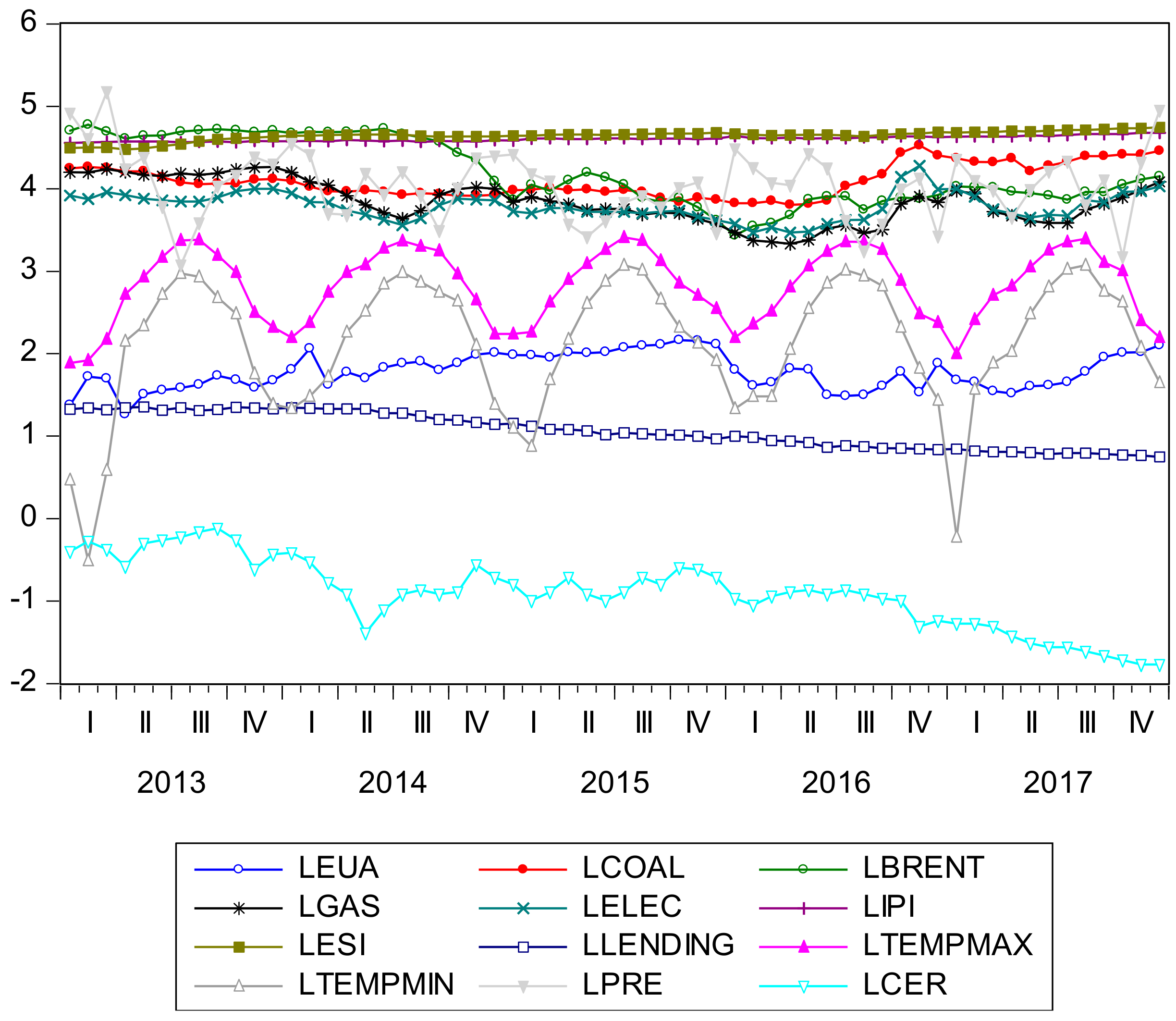
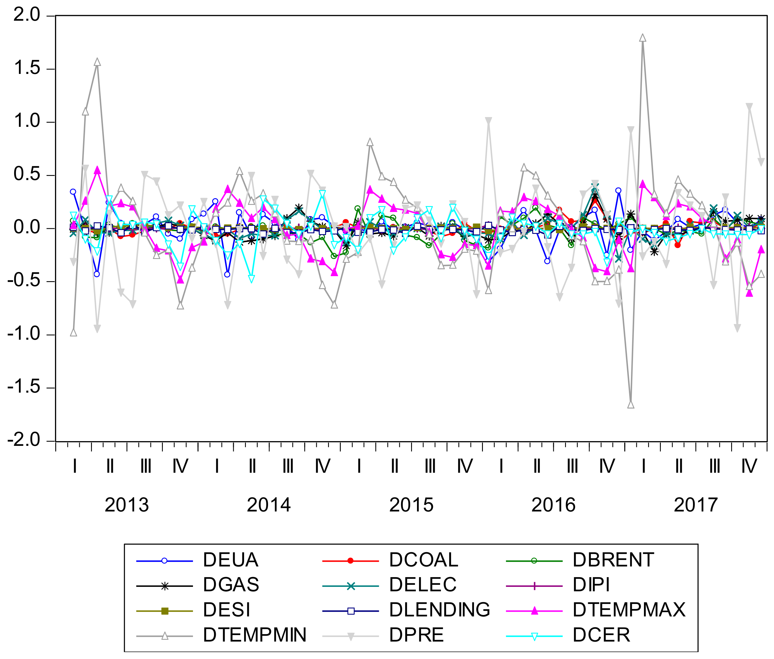
4.1.2. Data Statistics

The basic statistics provide the basis for the later discussion on the price determinants of European allowances. In addition, we use a descriptive analysis, natural log graph, discrete log graph, and correlations to show the background of the data.

However, we first present a macroeconomics time-series model. There are two approaches to explain this model. The first is the econometric approach, which sets the model based on the theoretical relationship between the dependent and independent variables. The basic theory behind it is the dynamic stochastic general equilibrium (DSGE) model and is defined as follows:

$${\mathrm{Y}}_{\mathrm{t}}={\mathsf{\beta }}_0+{\mathsf{\beta }}_1{\mathrm{X}}_{1\mathrm{t}}+{\mathsf{\beta }}_2{\mathrm{X}}_{2\mathrm{t}}+\cdots +{\mathsf{\beta }}_{\mathrm{k}}{\mathrm{X}}_{\mathrm{kt}}+{\mathsf{\epsilon }}_{\mathrm{t}}.$$

The second approach is the time-series approach, where we set the model based on the variables time flow characteristics. Therefore, we use variables that include past information and predict future movements. The basic theory behind it is the structural vector auto regressive (SVAR) model, defined as follows:

$${\mathrm{Y}}_{\mathrm{t}}=\mathsf{\delta }+{\mathsf{\alpha }}_1{\mathrm{Y}}_{\mathrm{t}-1}+{\mathsf{\alpha }}_2{\mathrm{Y}}_{\mathrm{t}-2}+\cdots +{\mathsf{\alpha }}_{\mathrm{p}}{\mathrm{Y}}_{\mathrm{t}-\mathrm{p}}+{\mathsf{\epsilon }}_{\mathrm{t}}.$$

The time-series approach has advantages and disadvantages. The disadvantage is that it only considers the times series in the variables, and so has weak explanatory power on the theoretical relationship between them. The advantage is that it is very useful and convenient for predicting target values [35].

Here, it is necessary to understand the natural log and discrete log, otherwise errors may occur. We use the natural log because it is time additive and follows a normal distribution. Therefore, in the time series, we can input the natural log to see how the value moves over time. However, even though it includes the time series, the data and variables are normally not stationary (i.e., they lack mean-reverting characteristics). The non-stationary condition is also time-varying and has a unit root. In addition, the variance and covariance are not finite constant. On the other hand, stationary data mean-reverting characteristics are not time-varying and do not have a unit root. Furthermore, the mean, variance, and covariance are finite constant [36]. Lee [35] states that if we use non-stationary time series variables without changing them to stationary time series by using the discrete log, then the t-value will increase with the sample size, despite having no correlation in reality. This problem is called a “spurious regression”. Most economic time series have spurious regressions and the non-stationary characteristic of a unit root. To avoid this problem, we input the discrete log and differentiate the data, changing it to a stationary time series, which means we can use the regression model. The ADF and PP tests can be used to find out if it has a unit root (non-stationary) or not (stationary).

For the descriptive analysis, we use the raw data (see

Table 2. The descriptive analysis of the raw data.

Variables	EUA	COAL	BRENT	GAS	ELEC	IPI	ESI	LENDING	TEMPMAX	TEMPMIN	PRE	CER
Mean	6.0983	61.2340	71.7890	48.2921	44.8217	100.0800	104.1367	2.9760	18.3167	10.6467	62.0748	0.4432
Median	5.9350	57.0600	57.4900	45.9720	43.2300	100.1000	105.0000	2.8150	18.1000	9.9000	58.8050	0.4100
Maximum	8.7100	92.4400	118.5800	71.0260	72.0400	107.5000	115.1000	3.8700	30.2000	21.60000	176.9700	0.890000
Minimum	3.540000	44.90000	31.01000	27.97500	32.06000	95.20000	88.20000	2.110000	6.600000	0.600000	21.69000	0.170000
Std. Dev.	1.314278	12.74857	28.33999	12.48789	7.680847	3.143721	6.044916	0.632164	7.373824	6.236510	28.20096	0.182659
Skewness	0.282000	0.692137	0.412412	0.289248	0.808002	0.516530	−1.072820	0.180262	0.099909	0.189441	1.654291	0.607750
Kurtosis	2.003380	2.274456	1.477453	1.964514	4.290711	2.451936	4.120893	1.461592	1.663493	1.751858	7.175078	2.708939
Jarque-Bera	3.278373	6.106573	7.496209	3.517219	10.69351	3.418962	14.65043	6.241694	4.565448	4.253525	70.94499	3.905387
Probability	0.194138	0.047204	0.0236	0.172284	0.004764	0.180960	0.000659	0.044120	0.102006	0.119223	0.00000	0.141891
Sum	365.9000	3674.040	4307.340	2897.526	2689.300	6004.800	6248.200	178.5600	1099.000	638.8000	3724.490	26.59000
Sum Sq.Dev.	101.9122	9589.034	47386.15	9200.898	3480.730	583.0960	2155.919	23.57824	3208.23	2249.749	46922.35	1.968498
Observations	60	60	60	60	60	60	60	60	60	60	60	60

). To interpret these data, we examine the skewness, which measures the degree of asymmetry of the series. ESI is negatively skewed, showing a long left tail, and PRE is positively skewed, showing a long right tail. Kurtosis measures the peakness or flatness of the distribution of the series. Here, PRE has a kurtosis value of 7.7175, which is more than 3, and so it has a peaked curve. We do not use the DSGE model to explain the theoretical relationships between the variables. Therefore, we do not explain the theoretical relationship using probability.

Second, Figure 2 and Figure 3 illustrate the natural log graphs and discrete log graphs, respectively. It seems reasonable to assume that Figure 2 reflects non-stationary data or variables that have a unit root. For the discrete log, the data change to stationary data, or variables that have no unit roots. This is because Figure 2 seems not to be mean reverting, whereas Figure 3 is. However, this is just an observation. The unit-root tests in Section 4.2 identify the stationarity clearly.

Third, as illustrated in

Table 3. Correlation analysis.

Variables	DEUA	DCOAL	DBRENT	DGAS	DELEC	DIPI	DESI	DLENDING	DTEMPMAX	DTEMPMIN	DPRE	DCER
DEUA	1
DCOAL	−0.0123	1
DBRENT	0.1828	0.0140	1
DGAS	−0.0002	0.4264	0.2904	1
DELEC	−0.0979	0.6142	0.1147	0.8226	1
DIPI	−0.0168	0.0369	−0.1650	0.1563	0.1632	1
DESI	0.4072	0.0211	0.1755	0.0616	0.0324	−0.1160	1
DLENDING	−0.0075	0.0602	−0.0684	−0.1223	−0.1191	0.0439	0.0113	1
DTEMPMAX	−0.0997	−0.2234	0.1764	−0.4053	−0.2891	−0.2111	−0.0841	−0.1060	1
DTEMPMIN	−0.1510	−0.1788	0.0287	−0.2968	−0.1577	−0.1014	−0.0954	−0.1267	0.8353	1
DPRE	0.0407	0.0776	−0.0762	0.1322	0.1289	0.2574	0.0133	0.1067	−0.4918	−0.3473	1
DCER	0.5234	−0.0848	0.0842	0.0151	−0.0550	−0.2785	0.1732	−0.1451	0.0999	−0.0002	−0.0464	1

, we use a correlation analysis for each variable. It does not give accurate and specific correlations or regressions, but is used to define a mathematical correlation between variables. To see the real correlation or relationship, a regression analysis should be used.

Table 3 shows that COAL, GAS, ELEC, IPI, LENDING, TEMPMAX, and TEMPMIN have a negative correlation with the EUA. Conversely, BRENT, ESI, PRE, and CER have a positive correlation. The biggest correlation with the EUA is that of CER (0.523). Normally, a value less than 0.2 means there is no correlation, 0.2–0.4 reflects a small correlation, 0.4–0.6 is a normal correlation, 0.6–0.8 is a high correlation, and more than 0.8 is a very high correlation. Therefore, most of the variables have little correlation or a normal correlation with the EUA.

4.1.3. VECM Model

In the time-series model, the basic theory is that of the SVAR model, which includes the widely used vector autoregression (VAR). The VAR model is a multivariate time-series model that combines time series and regression analysis features. Therefore, it is able to assume a correlation and casual relationship between many variables and is useful because it does not require economic theory. It simply explains the relationships between the variables as follows:

$${\mathrm{Y}}_{\mathrm{t}}={\mathsf{\alpha }}_1{\mathrm{Y}}_{\mathrm{t}-1}+{\mathsf{\alpha }}_2{\mathrm{Y}}_{\mathrm{t}-2}+\cdots +{\mathsf{\alpha }}_{\mathrm{p}}{\mathrm{Y}}_{\mathrm{t}-\mathrm{p}}+{\mathsf{\beta }\mathrm{X}}_{\mathrm{t}}+{\mathsf{\epsilon }}_{\mathrm{t}}.$$

The VAR model does not include a cointegration relationship, and regards cointegration as a setting error that creates a spurious regression. Therefore, in the VAR model, cointegration is also transformed using the discrete log. However, recent studies have indicated that it may be worth including the cointegration and not transforming it. Kim and Jang [36] state that if the variables have a cointegration relationship, but the researcher is only concerned about a spurious regression, transforming the data and using the VAR model may mean losing important information about the long-term relationships between the variables.

Cointegration is an important factor that should be explored. In financial time series, non-stationary time series often have a deterministic or stochastic trend. The basic meaning of cointegration in a time series is “a long-term equilibrium”, which is similar to a “trend”. This is because trends are long-term time series patterns. Therefore, if time-series variables or data have cointegration, then the variables share common trends. Thus, we can eliminate the stochastic trend and make it a real trend.

The VECM is a similar model, but it includes the cointegration relationship. It gradually adjusts variables that deviate from the long-term equilibrium using the error correction term (ECT) through a short-term adjustment process. Therefore, the difference between the VAR model and the VECM is the use of the ECT, which makes it possible to include the cointegration. Thus, it is justifiable to conclude that, for a non-stationary time series with cointegration, we should use the VECM rather than the VAR model. The basic VECM is defined as follows, where the variables on the right-hand side are all ECT, which becomes zero in the long term:

$$\Delta {\mathrm{Y}}_{1\mathrm{t}}={\mathsf{\alpha }}_1\left({\mathrm{Y}}_{2\mathrm{t}-1}-{\mathsf{\beta }\mathrm{Y}}_{1\mathrm{t}-1}\right)+{\mathsf{\epsilon }}_{1\mathrm{t}}$$

$$\Delta {\mathrm{Y}}_{2\mathrm{t}}={\mathsf{\alpha }}_2\left({\mathrm{Y}}_{2\mathrm{t}-1}-{\mathsf{\beta }\mathrm{Y}}_{1\mathrm{t}-1}\right)+{\mathsf{\epsilon }}_{2\mathrm{t}}.$$

Therefore, there are the two conditions to using the VECM. Firstly, if we input the natural log of non-stationary time series data, it should include cointegration. Secondly, if we first differentiate the non-stationary time series data, it should be changed to become stationary data.

The first condition is included because the VECM model should include the cointegration relationships, unless this results in the loss of long-term equilibrium information. The second condition ensures that we avoid the spurious regression problem by differentiating data with a cointegration relationship using the discrete log.

We use the VECM for two reasons. In Section 4.1.2 and in Figure 2 and Figure 3, we assumed the data were non-stationary time series when using the natural log. However, when we used the discrete log, the data changed to stationary data. This is evidence of the second condition of the VECM model.

This study is based on the work of Lee and Pak [25] and Cho [26], who use the VECM model to investigate the first two phases of the EU ETS. Since cointegration has a long-term equilibrium, it seems reasonable to assume that it will continue in the third phase.

However, we need to use unit-root tests and a cointegration test to verify whether the VECM is an appropriate choice (see Section 4.2.2 and Section 4.2.3.). Thus, if we input the discrete log data into the VECM and differentiate the data, but it does not seem stationary, or if we input the natural log of the non-stationary time series, but it does not show a cointegration relationship, then we should return to using the VAR model (the unit-root test and cointegration test confirm that the VECM model is appropriate).

The method of least squares is used for the VECM model because the maximum likelihood estimation method is usually used for the VAR model and requires that the data follow a normal distribution.

The VECM is set up based on Cho [26], who also uses monthly data to find the price determinants of EU ETS allowances using the VECM model. We also consider that some variables will be added, but not used. Equation (1) shows the VECM model regression equation. Here, $\Delta {\mathrm{Y}}_{\mathrm{t}}^{\mathrm{A}}$ is the EUA increase rate at t, $\Delta {\mathrm{Y}}_{\mathrm{t}}^{\mathrm{C}}$ is the COAL increase rate at t, $\Delta {\mathrm{Y}}_{\mathrm{t}}^{\mathrm{B}}$ is the Brent increase rate at t, $\Delta {\mathrm{Y}}_{\mathrm{t}}^{\mathrm{G}}$ is the Gas increase rate at t, $\Delta {\mathrm{Y}}_{\mathrm{t}}^{\mathrm{E}}$ is the ELEC increase rate at t, $\Delta {\mathrm{Y}}_{\mathrm{t}}^{\mathrm{I}}$ is the IPI increase rate at t, $\Delta {\mathrm{Y}}_{\mathrm{t}}^{\mathrm{S}}$ is the ESI increase rate at t, $\Delta {\mathrm{Y}}_{\mathrm{t}}^{\mathrm{L}}$ is the LENDING increase rate at t, $\Delta {\mathrm{Y}}_{\mathrm{t}}^{\mathrm{X}}$ is the TEMPMAX increase rate at t, $\Delta {\mathrm{Y}}_{\mathrm{t}}^{\mathrm{N}}$ is the TEMPMIN increase at t, $\Delta {\mathrm{Y}}_{\mathrm{t}}^{\mathrm{P}}$ is the PRE increase at t, and $\Delta {\mathrm{Y}}_{\mathrm{t}}^{\mathrm{R}}$ is the CER increase at t. The ECT is an adjustment function that considers the long-term equilibrium if cointegration exists. Because the ECT does not discard data, it does not regard cointegration as a setting error. Therefore, by using an adjustment function, it removes the short-term error and includes long-term equilibrium information. The error term$\mathsf{\epsilon }$is included because the statistic needs to handle the data limitations or noise. Therefore, it considers all errors as an error term as an important part of the VECM model. The impulse response function is used to determine how the dependent variables respond to the error term of each variable. The forecast error variance decomposition determines the relative influence of the other variables’ error terms on the dependent variables. The coefficient ${\mathsf{\alpha }}_{\mathrm{i}}$ measures the speed of adjustment of the ith endogenous variable toward the equilibrium. When used by itself, it usually represents the variables’ adjustment functions. However, when combined as an ECT, it represents the adjustment function for all variables, because the cointegration is a multi-variable trend:

$$\begin{gathered} \Delta {\mathrm{Y}}_{\mathrm{t}}^{\mathrm{j}}={\mathsf{\alpha }}_0^{\mathrm{j}}+{\mathsf{\alpha }}^{\mathrm{A}}{\mathrm{ECT}}_{\mathrm{t}-1}+{\displaystyle \sum }_{\mathrm{i}=1}^{\mathrm{p}}\Delta {\mathrm{Y}}_{\mathrm{t}-\mathrm{i}}^{\mathrm{A}}+{\displaystyle \sum }_{\mathrm{i}=1}^{\mathrm{p}}\Delta {\mathrm{Y}}_{\mathrm{t}-\mathrm{i}}^{\mathrm{C}}+{\displaystyle \sum }_{\mathrm{i}=1}^{\mathrm{p}}\Delta {\mathrm{Y}}_{\mathrm{t}-\mathrm{i}}^{\mathrm{B}}+{\displaystyle \sum }_{\mathrm{i}=1}^{\mathrm{p}}\Delta {\mathrm{Y}}_{\mathrm{t}-\mathrm{i}}^{\mathrm{G}}+ \\ {\displaystyle \sum }_{\mathrm{i}=1}^{\mathrm{p}}\Delta {\mathrm{Y}}_{\mathrm{t}-\mathrm{i}}^{\mathrm{E}}+{\displaystyle \sum }_{\mathrm{i}=1}^{\mathrm{p}}\Delta {\mathrm{Y}}_{\mathrm{t}-\mathrm{i}}^{\mathrm{I}}+{\displaystyle \sum }_{\mathrm{i}=1}^{\mathrm{p}}\Delta {\mathrm{Y}}_{\mathrm{t}-\mathrm{i}}^{\mathrm{S}}+{\displaystyle \sum }_{\mathrm{i}=1}^{\mathrm{p}}\Delta {\mathrm{Y}}_{\mathrm{t}-\mathrm{i}}^{\mathrm{L}}+{\displaystyle \sum }_{\mathrm{i}=1}^{\mathrm{p}}\Delta {\mathrm{Y}}_{\mathrm{t}-\mathrm{i}}^{\mathrm{X}}+{\displaystyle \sum }_{\mathrm{i}=1}^{\mathrm{p}}\Delta {\mathrm{Y}}_{\mathrm{t}-\mathrm{i}}^{\mathrm{N}}+ \\ {\displaystyle \sum }_{\mathrm{i}=1}^{\mathrm{p}}\Delta {\mathrm{Y}}_{\mathrm{t}-\mathrm{i}}^{\mathrm{P}}+{\displaystyle \sum }_{\mathrm{i}=1}^{\mathrm{p}}\Delta {\mathrm{Y}}_{\mathrm{t}-\mathrm{i}}^{\mathrm{R}}+{\mathsf{\epsilon }}_{\mathrm{t}}^{\mathrm{j}}, \mathrm{where} \mathrm{j} = \mathrm{A}, \mathrm{C}, \mathrm{B}, \mathrm{G}, \mathrm{E}, \mathrm{I}, \mathrm{S}, \mathrm{L}, \mathrm{X}, \mathrm{N}, \mathrm{P}, \mathrm{R}. \end{gathered}$$

(1)

The equation above shows the determinants of each variable through the VECM model equation. We set the EUA price as the dependent variable, and use past data on the EUA price and the other variables as explanatory variables. The equation shows the EUA price determinants and the determinants of the other variables. For example, $\Delta {\mathrm{Y}}_{\mathrm{t}}^{\mathrm{j}}$ denotes the current EUA price (at time t), ${\mathsf{\alpha }}_0^{\mathrm{j}}$ is the EUA price-adjustment function, and ${\mathsf{\alpha }}^{\mathrm{j}}{\mathrm{ECT}}_{\mathrm{t}-1}$ is the ECT of each variable. Then, ${\displaystyle \sum }_{\mathrm{i}=1}^{\mathrm{p}}\Delta {\mathrm{Y}}_{\mathrm{t}-\mathrm{i}}^{\mathrm{j}}$ shows the past data of the EUA price (at time t − i), ${\displaystyle \sum }_{\mathrm{i}=1}^{\mathrm{p}}\Delta {\mathrm{Y}}_{\mathrm{t}-\mathrm{i}}^{\mathrm{j}}$ shows the past data for the coal price (at time t − i), and so on. Lastly, ${\mathsf{\epsilon }}_{\mathrm{t}}^{\mathrm{j}}$is the error term for the EUA price (at time t).

The basic sequence of the research process is illustrated in

Table 4. Empirical results sequences preview.

Sequences	Issues	Analysis Methods	Using Variables
1	Check the correct Lag order	SIC	Natural log
2	Check the time series stationarity	Unit-root test & ADF, PP Test	Natural log & Discrete log
3	Check the cointegration	Johansen Cointegration	Natural log
4	Find out the causality	Granger Causality Test	Discrete log
5	Measure the correlation	VECM estimation & Impulse Response Function	Natural log
6	Compare the relative correlation size	Forecast Error Variance Decomposition	Natural log

. There are six steps. First, we use the SIC to find the right lag order. Here, the natural log variables are used. Second, we test for unit roots using the ADF and PP tests to find out if the variables are stationary or non-stationary. We use both the natural log and discrete log for the variables. Third, we use the Johansen cointegration test to find out if the variables contain cointegration. Here, we only use the natural log of the data. Fourth, we use the Granger causality test to find which variables have a causality relationship with the EUA price. This step uses the discrete log only. Fifth, we use the VECM estimation and the impulse response function to measure the accurate relationship between the EUA price and the other variables, using the natural log. Finally, we use the forecast error variance decomposition to compare the size of the correlation between the EUA price and the other variables. As in the fifth step, we use the natural log only. Note that the fifth and sixth steps should use the discrete log for the data, because a time-series regression requires stationary data. However, EViews employs the natural log owing to its systematically changing functions.

This process enables us to investigate which variables affect the EUA price in Phase 3 of the EU ETS, as well as to verify the findings of previous studies.

4.2. Empirical Results

4.2.1. Lag-Order Selection Criteria

The lag length is an important part of the autoregressive (AR) process because it shows how far back we need to go to ensure a stable size for the test and to minimize lost power.

The VAR and VECM models choose the lag length in the same way as in the AR process, namely, using information criteria. Here, the lower the values of the information criteria, the more appropriate the lag is.

Two criteria are commonly used: Akaike’s information criterion (AIC) and the SIC. Cho [26] uses the AIC to find an appropriate lag length. However, in a small sample, the AIC contains bias in the measurement of the actual time difference. Therefore, we use the SIC to find the right lag length [37]. The formula for the SIC is as follows:

$$\mathrm{SIC}\left(\mathrm{p}\right)=\ln \left|{\mathsf{\Omega }}_{\mathrm{p}}\right|+\frac{\ln \left(\mathrm{T}\right)}{\mathrm{T}}{\mathrm{pK}}^2.$$

In this function, T denotes the number of observations, K is the number of dependent variables, ${\mathsf{\Omega }}_{\mathrm{p}}$ is the time difference, and p is the result of the variance and covariance process.

Next, we need to decide whether to use the natural log or discrete log for the variables. As discussed, the natural log has a time additive characteristic in non-stationary data. The discrete log uses the natural log (non-stationary data) and transforms the data to make it a stationary time series. In this case to choose the right lag length, the data should be time additive (not transformed). Therefore, we use the natural log and the SIC to find an appropriate lag length.

The results are shown in

Table 5. Lag-order selection criteria.

Lag	LogL	LR	FPE	AIC	SC	HQ
0	518.4073	N/A	3.12 × 10−23	−17.76868	−17.33856	−17.60152
1	1093.468	887.8132	9.28 × 10−30	−32.89362	−27.30211 *	−30.72057
2	1280.879	210.4257	3.94 × 10−30	−34.41679	−23.66389	−30.23785
3	1531.401	175.8054 *	8.70 × 10−31 *	−38.15443 *	−22.24014	−31.96959 *

* indicates lag order selected by the criterion.

. The lowest SIC value occurs for a lag of 1 (−27.30211). Therefore, this is the lag length employed here.

4.2.2. Unit-Root Test

The unit-root test is based on proving the null hypothesis ${\mathrm{H}}_0:\mathsf{\delta }=0$, which means there is a unit root. The alternative hypothesis is ${\mathrm{H}}_0:\mathrm{p}<1{ \mathrm{or} \mathrm{H}}_1:\mathsf{\delta }<0$, which shows there is no unit root. Therefore, if $\mathsf{\delta }$ is greater than or equal to zero, there is a unit root. In addition, the unit-root test is a one-tail test. It does not include the relationship between the variables. Instead, it simply determines whether a unit root exists.

There are two methods for testing the stationarity of a time series: the ADF and PP unit-root tests. The three equations for the ADF test are as follows:

$$\Delta {\mathrm{Y}}_{\mathrm{t}}={\mathsf{\delta }\mathrm{Y}}_{\mathrm{t}-1}+{\mathsf{\alpha }}_1\Delta {\mathrm{Y}}_{\mathrm{t}-1}+\cdots +{\mathsf{\alpha }}_{\mathrm{p}}\Delta {\mathrm{Y}}_{\mathrm{t}-\mathrm{p}}+{\mathsf{\epsilon }}_{\mathrm{t}}$$

$$\Delta {\mathrm{Y}}_{\mathrm{t}}=\mathrm{Y}+{\mathsf{\delta }\mathrm{Y}}_{\mathrm{t}-1}+{\mathsf{\alpha }}_1\Delta {\mathrm{Y}}_{\mathrm{t}-1}+\cdots +{\mathsf{\alpha }}_{\mathrm{p}}\Delta {\mathrm{Y}}_{\mathrm{t}-\mathrm{p}}+{\mathsf{\epsilon }}_{\mathrm{t}}$$

$$\Delta {\mathrm{Y}}_{\mathrm{t}}=\mathrm{Y}+\mathsf{\beta }\mathrm{t}+{\mathsf{\delta }\mathrm{Y}}_{\mathrm{t}-1}+{\mathsf{\alpha }}_1\Delta {\mathrm{Y}}_{\mathrm{t}-1}+\cdots +{\mathsf{\alpha }}_{\mathrm{p}}\Delta {\mathrm{Y}}_{\mathrm{t}-\mathrm{p}}+{\mathsf{\epsilon }}_{\mathrm{t}}.$$

The difference between the two tests is that, in the PP test, the $\mathsf{\tau }$ statistics are adjusted. Here, we use both.

The results are shown in

Table 6. Unit-root test results—Natural log (L).

	ADF		PP
	p-Value	t-Statistic	p-Value	t-Statistic
LEUA	0.0356	−3.055988	0.0422	−2.984378
LCOAL	0.6827	−1.167349	0.7379	−1.027621
LBRENT	0.5959	−1.359506	0.5579	−1.437604
LGAS	0.2579	−2.068355	0.3568	−1.842875
LELEC	0.0599	−2.833176	0.1257	−2.479064
LIPI	0.9961	0.9997	0.103632	0.9634
LESI	0.2928	−1.984367	0.3421	−1.874023
LLENDING	0.9035	−0.389219	0.9718	0.221042
LTEMPMAX	0.00111	−3.529973	0.0139	−3.425476
LTEMPMIN	0.0000	−5.841264	0.00136	−3.433459
LPRE	0.0001	−5.030188	0.0004	−4.622699
LCER	0.7961	−0.853044	0.8835	−0.499416

and

Table 7. Unit-root test results—Discrete log (D).

	ADF		PP
	p-Value	t-Statistic	p-Value	t-Statistic
DEUA	0.0000	−9.758254	0.0000	−10.71395
DCOAL	0.0000	−5.584956	0.0000	−5.597697
DBRENT	0.0000	−5.961247	0.0000	−5.992281
DGAS	0.0001	−5.04162	0.0001	−4.976623
DELEC	0.0000	−5.86215	0.0000	−5.86215
DIPI	0.0000	−8.654458	0.0000	−12.33428
DESI	0.0001	−4.953879	0.0001	−4.952978
DLENDING	0.0343	−3.073978	0.0000	−9.62994
DTEMPMAX	0.0000	−8.081471	0.003	−3.972452
DTEMPMIN	0.0000	−6.295002	0.0000	−6.431096
DPRE	0.0000	−9.445539	0.0000	−13.173262
DCER	0.0000	−7.758334	0.0000	−8.75748

. Table 6 shows that the natural log input data are non-stationary, because most of the variables have p-values below the 5% level. In contrast, Table 7 shows that the discrete log input data are stationary because the variables all reject the null hypothesis of a unit root. Therefore, this result satisfies the second condition of the VECM model (that the data are non-stationary, but if differentiated using the discrete log, they become stationary).

4.2.3. Cointegration Test

Before discussing the hypotheses and the results, we need to revisit the meaning of cointegration. This is because we found several errors in previous studies where the researchers applied the theory incorrectly. Unfortunately, because this study is based on Lee and Pak [25] and Cho [26], it contains the same errors.

The purpose of the cointegration test is to find cointegration in non-stationary time series. In addition, it differs from the unit-root test because the latter is a one-tailed test, whereas the cointegration test is two-tailed test. As discussed in Section 4.1.3, time series data usually contain non-stationary data, where the variables have a stochastic trend with each other. In addition, the cointegration test can determine whether the data have a long-term equilibrium and share common long-term trends. Therefore, if the variables contain cointegration, the stochastic trends have changed to a real trend, in which case, the cointegration test should use the non-stationary time series that adds time (natural log). This is because if differentiated data are used and transformed, then despite the cointegration, we cannot be sure that they originally contained cointegration, in which case, the result of using the discrete log may differ from that using the original data.

However, after finding a unit root, some researchers use the discrete log and change the data to a stationary time series to avoid spurious regressions, using the stationary data in the cointegration test. For example, in Lee and Pak [25] and Cho [26], the researchers stated that they could not find any cointegration when using the natural log. However, after using the discrete log, they did find cointegration, and so used the VECM model. This is a serious error because the stationary data are not natural data (they are transformed by the discrete log). Needless to say, the results then become problematic. Therefore, in a cointegration test, the natural log of the variables must be used, not the discrete log. This is because the purpose of the test is to find common trends in the non-stationary time series variables, and so we cannot transform the data.

The basic model of the cointegration test is defined as below. In this equation, the null hypothesis is ${\mathrm{H}}_0:\mathsf{\alpha }=\mathsf{\beta }=\mathrm{Y}=0$. If the null hypothesis is rejected, then it is appropriate to conclude that the variables contain cointegration:

$$\Delta {\mathrm{Y}}_{\mathrm{t}}=\mathsf{\alpha }+\mathsf{\beta }\mathrm{t}+{\mathrm{Yy}}_{\mathrm{t}-1}+{\displaystyle \sum }_{\mathrm{i}=1\to \mathrm{t}}{\mathsf{\delta }}_{\mathrm{i}}\Delta {\mathrm{y}}_{\mathrm{t}-1}+{\mathsf{\epsilon }}_{\mathrm{t}}.$$

The Johansen cointegration test is the most recognized test. Kim and Jang [37] state that it is easy to understand it as an expanded version of the ADF test, where it expands the one-tailed test to a two-tailed test. The basic model of the Johansen cointegration test is defined below, where the null hypothesis is ${\mathrm{H}}_0:\mathrm{rank}(П)\le \mathrm{r},{ \mathrm{H}}_1:\mathrm{rank}(П)\ge \mathrm{r}+1$:

$$\Delta {\mathrm{Y}}_{\mathrm{t}}={{\displaystyle \prod }}^{}{\mathrm{Y}}_{\mathrm{t}-1}+{\mathrm{A}}_1^{*}\Delta {\mathrm{Y}}_{\mathrm{t}-1}+{\mathrm{A}}_2^{*}\Delta {\mathrm{Y}}_{\mathrm{t}-2}+\cdots {\mathrm{A}}_{\mathrm{p}-1}^{*}\Delta {\mathrm{Y}}_{\mathrm{t}-\mathrm{p}+1}+{\mathsf{\epsilon }}_{\mathrm{t}}$$

$${ \mathrm{A}}_{\mathrm{j}}^{*}=-\left({\mathrm{A}}_{\mathrm{j}+1}+{\mathrm{A}}_{\mathrm{j}+2}+\cdots {\mathrm{A}}_{\mathrm{p}}\right)$$

$${{\displaystyle \prod }}^{}={\mathrm{A}}_1+{\mathrm{A}}_2+\cdots +{\mathrm{A}}_{\mathrm{p}}-{\mathrm{l}}_{\mathrm{n}}.$$

Table 8. Johansen cointegration test (trace results).

Unrestricted Cointegration Rank Test (Trace)
Hypothesized No. of CE(s)	Eigenvalue	Trace Statistic	0.05 Critical Value	Prob. **
None *	0.8763	504.6197	334.9837	0.0000
At most 1 *	0.7711	383.3907	285.1425	0.0000
At most 2 *	0.6785	297.8750	239.2354	0.0000
At most 3 *	0.6197	232.0668	197.3709	0.0003
At most 4 *	0.5279	175.9949	159.5297	0.0046
At most 5 *	0.4738	132.4601	125.6154	0.0179
At most 6	0.3973	95.22120	95.75366	0.0544
At most 7	0.3846	65.85029	69.81889	0.0995
At most 8	0.2759	37.69285	47.85613	0.3156
At most 9	0.1792	18.97090	29.79707	0.4950
At most 10	0.1216	7.519811	15.49471	0.5181
At most 11	5.19 × 10−5	0.003010	3.841466	0.9547

Trace test indicates 6 cointegrating eqn(s) at the 0.05 level; * denotes rejection of the hypothesis at the 0.05 level; ** MacKinnon-Haug-Michelis (1999) p-values.

and

Table 9. Johansen cointegration test (maximum eigenvalue).

Unrestricted Cointegration Rank Test (Maximum Eigenvalue)
Hypothesized No. of CE(s)	Eigenvalue	Trace Statistic	0.05 Critical Value	Prob. **
None *	0.8763	121.2290	76.5784	0.0000
At most 1 *	0.7711	85.5157	70.5351	0.0012
At most 2 *	0.6785	65.8082	64.5047	0.0373
At most 3	0.6197	56.0719	58.4335	0.0840
At most 4	0.5279	43.5349	52.3626	0.2978
At most 5	0.4738	37.2389	46.2314	0.3274
At most 6	0.3973	29.3709	40.0776	0.4659
At most 7	0.3846	28.1574	33.8769	0.2063
At most 8	0.2759	18.7220	27.5843	0.4363
At most 9	0.1792	11.4511	21.1316	0.6023
At most 10	0.1216	7.5168	14.2646	0.4299
At most 11	0.0001	0.0030	3.8415	0.9547

Trace test indicates 3 cointegrating eqn(s) at the 0.05 level; * denotes rejection of the hypothesis at the 0.05 level; ** MacKinnon-Haug-Michelis (1999) p-values.

show the results. In Table 8, the trace results of the Johansen cointegration test reject the null hypothesis of no cointegration. The results also reject the hypothesis of less than five cointegrating vectors (${\mathrm{H}}_0:\mathrm{r}\le 5$), with a p-value of less than 5%; thus, the variables have at least five cointegrating vectors. In Table 9, the maximum eigenvalue results reject the null hypothesis of no cointegration (in this case, it rejects the hypothesis of less than two cointegrating vectors, ${\mathrm{H}}_0:\mathrm{r}\le 2$, by less than 5%, which means the variables have at least two cointegrating vectors). These results are interesting because the trace cointegration result and the maximum eigenvalue cointegration result are different. Here, EViews allows us to choose only one case. However, both results reject the null hypothesis of no cointegration.

In this section, we have identified an error in previous studies related to the cointegration test, which brings their results into question. Second, we determined that the variables contain cointegration by using the Johansen cointegration test. Therefore, we choose to use the VECM model because both conditions for using the model are satisfied.

4.2.4. Granger Causality Test

In this section, we conduct regression analysis using the Granger Causality test, VECM estimation, impulse response function, and forecast error variance. The results will show the causality between the variables and the EUA price, and will enable us to compare the third phase of the EU ETS with the third phase in terms of the determinants of the price.

The basic logic of the Granger causality test is that when predicting Y, if using past data for Y and X is more valuable than using the past data of Y only, then X Granger-causes Y, and we can assume that X causes Y. Conversely, when predicting X, if using past data for both X and Y is more valuable than using the past data for X only, then Y Granger-causes X, and we can assume Y causes X. If both sides of the relationship exist, this is called interdependence.

The null hypothesis of the Granger causality test is that the first variable does not Granger-cause the second variable. If this is rejected, then the first variable causes the second variable. The model of the Granger causality test is given below. Note that we need to use a stationary time series because this is a regression test.

$${\mathrm{y}}_{\mathrm{t}}={\displaystyle \sum }_{\mathrm{i}=1\to \mathrm{p}}{\mathsf{\alpha }}_{\mathrm{i}}{\mathrm{X}}_{\mathrm{t}-\mathrm{i}}+{\displaystyle \sum }_{\mathrm{j}=1\to \mathrm{p}}{\mathsf{\beta }}_{\mathrm{j}}{\mathrm{y}}_{\mathrm{t}-\mathrm{j}}+{\mathsf{\epsilon }}_{1\mathrm{t}}$$

$${\mathrm{x}}_{\mathrm{t}}={\displaystyle \sum }_{\mathrm{i}=1\to \mathrm{n}}{\mathrm{Y}}_{\mathrm{i}}{\mathrm{X}}_{\mathrm{t}-\mathrm{i}}+{\displaystyle \sum }_{\mathrm{j}=1\to \mathrm{p}}{\mathsf{\delta }}_{\mathrm{j}}{\mathrm{y}}_{\mathrm{t}-\mathrm{j}}+{\mathsf{\epsilon }}_{2\mathrm{t}}.$$

Table 10. Granger causality test results *** 1% ** 5%.

	Y	DCOAL	DBRENT	DGAS	DELEC	DIPI	DESI	DLENDING	DTEMPMAX	DTEMPMIN	DPRE	DCER
X
DEUA		X ⇏ Y	X ⇏ Y	X ⇏ Y **	X ⇏ Y ***	X ⇏ Y	X ⇏ Y	X ⇏ Y	X ⇏ Y	X ⇏ Y	X ⇏ Y	X ⇏ Y
DEUA		Y ⇏ X	Y ⇏ X	Y ⇏ X	Y ⇏ X	Y ⇏ X	Y⇏X	Y ⇏ X	Y ⇏ X	Y ⇏ X	Y ⇏ X	Y ⇏ X

shows the Granger causality test results. The results show that DEUA ⇏ DELEC *** and DEUA ⇏ DGAS **. This implies that these variables reject the null hypothesis at the 1% and 5% levels, showing one-sided causality. In particular, EUA Granger-causes ELEC has the strongest one-sided causality. Furthermore, EUA Granger-causes GAS is also strong. We can interpret that EUA Granger-causes ELEC as follows Boersen and Scholtens [38]: if the EUA futures price increases or decreases, it causes a corresponding change in the fuel price (if the EUA price increases, then companies have to pay a higher allowance price, and so use less fuel. If the price decreases, then companies find it easier to pay the allowance price, and so use more fuel). As a result, the electricity price is determined by the cost of fuel inputs, and so has a causal relationship with the allowance price. We can interpret EUA Granger-causing GAS as in Lee [39]: if the EUA price and using high carbon-emission fuels (e.g., coal) is cheaper than buying natural gas, companies will not use natural gas, and will instead buy allowances and use coal or oil. Therefore, if the EUA price increases or decreases, companies will use more or less natural gas, respectively. Thus, the natural gas price has a causal relationship with the allowance price.

Table 11. Comparison between Granger causality test results *** 1% ** 5%.

	[24] Phase 1 and 2	[25] Phase 2	Present Study Phase 3
DEUA ⇒ X	DEUA2 ⇒ DCOAL2 ** DEUA2 ⇒ DPOWER2 **	DEUA ⇒ DCER **	DEUA ⇒ DGAS ** DEUA ⇒ DELEC ***
X ⇒ DEUA	DOIL1 ⇒ DEUA1 ** DGAS ⇒ DEUA *** DPOWER2 ⇒ DEUA2 **	DCER ⇒ DEUA **

shows the results of our Granger causality test, as well as those of Lee and Pak [25] and Cho [26]. Recall that we focus on Phase 3, whereas Lee and Pak [25] examine the first and second phases of the EU ETS, and Cho [26] emphasizes the second phase of the EU ETS. Comparing the results, we find a marked contrast between the second and third phase. First, Lee and Pak [25] state that EUA2 and POWER2 are interdependent. Cho [26] finds interdependence between EUA and CER. However, in the third phase, this interdependence has disappeared, because we find only one side causalities: for example, EUA Granger-causes ELEC, or EUA Granger-causes GAS. Second, in Lee and Pak [25], OIL2 and COAL2 show a causality relationship until the second phase, but in the third phase this relationship disappears. Furthermore, the CER causality in the second phase becomes weaker. Third, the one-sided causalities of EUA Granger-causing GAS and EUA Granger-causing ELEC in the third phase become much stronger than they were before.

4.2.5. Estimation of the VECM and the Impulse Response Function

In this section, we use the VECM to find the price determinants of the EUA. Here, we measure the accurate correlation between the EUA price and the other variables. In Section 4.2.6, we use the forecast error variance decomposition to compare the relative correlation sizes that influence the EUA.

Before discussing the EUA price determinants, we need to revisit the research error identified earlier because it applies here as well.

In a regression test, non-stationary data need to be changed to stationary data. However, if a system provides a manual, then the researcher should follow the instructions set out there. This is not a matter of theoretical knowledge, but a problem of system utilization. EViews and STATA are statistics tools that provide such manuals, which means researchers need to understand how to use them correctly. If the researcher prefers to use their theoretical knowledge, GAUSS, MATLAB, and PYTHON are better options as statistics tool. In EViews, when using the VECM or VAR models, the software automatically differentiates the data by inputting the discrete log. Therefore, if the data have already been differentiated, they will be differentiated twice, as occurred in Lee and Pak [25] and Cho [26], which affects the results. Thus, when using EViews, we need to input the natural log data.

Next, we discuss the correlation between the EUA price and the variables identified by the VECM estimation and the impulse response function. Here, we explain the VECM estimation. We use the impulse response function to measure the accuracy of the correlation. We do not employ the results of the VECM estimation directly, because they are difficult to interpret (note that [25,26] choose to interpret the VECM estimation). Consequently, the main results described here are based on the impulse response function. In spite of its results being difficult to interpret, the VECM is necessary in order to use the impulse response function and forecast error variance decomposition.

The overall VECM test uses the method of least squares, defined below. Here, ${\mathrm{y}}_{1\mathrm{t} }{ \mathrm{and} \mathrm{y}}_{2\mathrm{t}}$ denote the same variables, but that change over time. The results are shown in

Table 12. Estimation of VECM, *** 1%, ** 5%, and * 10% prob.

Error Correction	D(LEUA)	D(LCOAL)	D(LBRENT)	D(LGAS)	D(LELEC)	D(LIPI)	D(LESI)	D(LLENDING)	D(LTEMPMAX)	D(LTEMPMIN)	D(LPRE)	D(LCER)
CoinEq1	−0.091056 **	−0.02909	−0.038545	−0.018906	0.0161	0.006234 ***	−0.011087 ***	−0.005795	0.066666	0.421580 ***	0.276651 **	−0.037974
	(0.04532)	(0.01963)	(0.02785)	(0.02674)	(0.02885)	(0.00247)	(0.0279)	(0.00524)	(0.05011)	(0.10041)	(0.12648)	(0.04828)
	[−2.00912]	[−0.14822]	[−1.38377]	[−0.70699]	[0.55732]	[2.52391]	[−3.97473]	[−1.10685]	[1.33048]	[4.19860]	[2.18725]	[−0.78658]
D(LEUA(−1))	−0.246435	−0.019550	0.009934	0.197111 *	0.190458 *	−0.007794	0.005463	−0.021163	−0.167448	−0.825691 **	0.144223	−0.174448
	(0.18171)	(0.07869)	(0.11168)	(0.10722)	(0.11568)	(0.00990)	(0.01118)	(0.02099)	(0.20089)	(0.40257)	(0.50711)	(0.19356)
	[−1.35622]	[−0.24846]	[0.08895]	[1.83844]	[1.64635]	[−0.78698]	[0.48843]	[−1.00824]	[−0.83352]	[−2.05104]	[0.28440]	[−0.90127]
D(LCOAL(−1))	−0.013725	0.261666	−0.118222	0.012572	0.221321	0.048508 **	−0.038056	−0.050976	0.220812	−0.248014	−1.753526	−0.336411
	(0.42726)	(0.18502)	(0.26260)	(0.25211)	(0.27202)	(0.02329)	(0.02630)	(0.04936)	(0.47237)	(0.94660)	(1.19241)	(0.45513)
	[−0.03212]	[1.41425]	[−0.45020]	[0.04987]	[0.81363]	[2.08314]	[−1.44713]	[−1.03282]	[0.46745]	[−0.26201]	[−1.47057]	[−0.73916]
D(LBRENT(−1))	0.215441	0.140627	0.321829 *	0.069447	0.057995	−0.012390	0.008501	−0.058681 *	0.113594	0.445976	0.785138	0.038809
	(0.27340)	(0.11839)	(0.16803)	(0.16132)	(0.17406)	(0.01490)	(0.01683)	(0.03158)	(0.30226)	(0.60571)	(0.76300)	(0.29123)
	[0.78801]	[1.18780]	[1.91528]	[0.43050]	[0.33319]	[−0.83156]	[0.50519]	[−1.85804]	[0.37581]	[0.73628]	[1.02901]	[0.13326]
D(LGAS(−1))	−0.389961	−0.046329	−0.238205	0.343399	0.158321	−0.001003	0.07493	0.002106	0.429552	0.155370	−1.638213	0.475428
	(0.48769)	(0.21119)	(0.29974)	(0.28776)	(0.31049)	(0.02658)	(0.03002)	(0.05634)	(0.53919)	(1.08049)	(1.36106)	(0.51950)
	[−0.79960]	[−0.21937]	[−0.79471]	[1.19333]	[0.50990]	[−0.03774]	[0.24964]	[0.03738]	[0.79667]	[0.14380]	[−1.20363]	[0.91516]
D(LELEC(−1))	0.206852	0.049393	0.015659	0.013596	0.130542	0.000634	−0.004748	0.019405	−0.781744	1.394452	2.088369	−0.359369
	(0.47924)	(0.20753)	(0.29454)	(0.28278)	(0.30511)	(0.02612)	(0.02950)	(0.05536)	(0.52984)	(1.06175)	(1.33746)	(0.51049)
	[0.43163]	[0.23801]	[0.05316]	[0.04808]	[0.42785]	[0.02426]	[−0.16098]	[0.35053]	[−1.47544]	[1.31335]	[1.56144]	[−0.70396]
D(LIPI(−1))	−0.525554	0.924336	0.987121	−1.465294	−0.305560	−0.364519 ***	0.067914	0.697356 ***	3.700777	8.8110889 *	7.621193	−1.806517
	(2.40413)	(1.04108)	(1.47760)	(1.41856)	(1.53060)	(0.13103)	(0.14797)	(0.27772)	(2.65796)	(5.32635)	(6.70948)	(2.56093)
	[−0.21860]	[0.88786]	[0.66806]	[−1.03294]	[−0.19963]	[−2.78203]	[0.45897]	[2.51104]	[1.39233]	[1.65424]	[1.13588]	[−0.70541]
D(LESI(−1))	−0.994048	−0.513154	0.387759	−0.572071	0.124768	0.285791 **	0.179288	0.725675 ***	−2.242645	2.401617	10.31127	−2.029063
	(2.30974)	(1.00021)	(1.41958)	(1.36287)	(1.47051)	(0.12588)	(0.14216)	(0.26681)	(2.55361)	(5.11723)	(6.44606)	(2.46038)
	[−0.43037]	[−0.51305]	[0.27315]	[−0.41976]	[0.08485]	[2.27031]	[1.26115]	[2.71979]	[−0.87823]	[0.46932]	[1.59962]	[−0.82469]
D(LLENDING(−1))	−0.244991	−0.336282	0.391066	−0.380389	−0.088921	0.003200	−0.033142	−0.275302 **	−0.15082	3.264887	4.254464	−1.280798
	(1.08889)	(0.47153)	(0.66924)	(0.64250)	(0.69325)	(0.05934)	(0.06702)	(0.12578)	(1.20386)	(2.41244)	(3.03889)	(1.15991)
	[−0.22499]	[−0.71317]	[0.58434]	[−0.59204]	[−0.12827]	[0.05392]	[−0.49450]	[−2.18868]	[−0.12475]	[1.35336]	[1.40001]	[−1.10422]
D(LTEMPMAX(−1))	0.211030	0.003397	0.144242	0.136085	0.061460	−0.019323	0.046989 ***	0.014126	0.904233 ***	1.236196	−1.799758 ***	0.125350
	(0.25144)	(0.10888)	(0.15453)	(0.14836)	(0.16008)	(0.01370)	(0.01548)	(0.02905)	(0.27798)	(0.55706)	(0.70171)	(0.26784)
	[0.83929]	[0.03120]	[0.93339]	[0.91725]	[0.38394]	[−1.41007]	[3.03631]	[0.48633]	[3.25282]	[2.21915]	[−2.56480]	[0.46801]
D(LTEMPMIN(−1))	−0.132595	0.007440	−0.036958	−0.058476	−0.007237	0.004188	−0.018677 ***	−0.003647	−0.103932	−0.116912	0.400062	−0.024429
	(0.09497)	(0.04113)	(0.05837)	(0.05604)	(0.06046)	(0.00518)	(0.00585)	(0.01097)	(0.10500)	(0.21041)	(0.26504)	(0.10116)
	[−1.39618]	[0.18092]	[−0.63318]	[−1.04353]	[−0.11970]	[0.80905]	[−3.19519]	[−0.33242]	[−0.98986]	[−0.55565]	[1.50943]	[−0.24148]
D(LPRE(−1))	−0.039022	0.020735	0.010080	0.025071	0.024911	−0.007271	0.001198	−0.009930	0.227571 ***	0.462331 ***	−0.537683 ***	0.033971
	(0.05427)	(0.02350)	(0.03335)	(0.03202)	(0.03455)	(0.00296)	(0.00334)	(0.00627)	(0.06000)	(0.12023)	(0.15146)	(0.05781)
	[−0.71904]	[0.88228]	[0.30221]	[0.78293]	[0.72099]	[−2.45833]	[0.35870]	[−1.58391]	[3.79288]	[3.84523]	[−3.55008]	[0.58764]
D(LCER(−1))	0.097043	0.020851	−0.102998	−0.051150	−0.012785	−0.0008846	−0.006234	0.013348	−0.211037	0.022758	0.200962	0.08337
	(0.17338)	(0.07508)	(0.10656)	(0.10230)	(0.11038)	(0.00945)	(0.01067)	(0.02003)	(0.19168)	(0.38411)	(0.48386)	(0.18468)
	[0.55973]	[0.27773]	[−0.96659]	[−0.5000]	[−0.15583]	[−0.08952]	[−0.58415]	[0.66648]	[−1.10098]	[0.05925]	[0.41553]	[0.04514]
C	0.016433	0.001411	−0.010603	−0.001009	−0.000152	0.001422	0.003159 **	−0.017318 ***	0.001768	0.051841	−0.003720	−0.020630
	(0.02498)	(0.01082)	(0.01536)	(0.01474)	(0.01591)	(0.00136)	(0.00154)	(0.00289)	(0.02762)	(0.05535)	(0.06972)	(0.02661)
	[0.65773]	[0.13043]	[−0.69049]	[−0.06842]	[−0.00956]	[1.04438]	[2.05402]	[−6.02149]	[0.06400]	[0.93659]	[−0.05335]	[−0.77518]

. The first value in the table is the estimated coefficient, the second is the standard error, and the third is the t-statistic.

$${\mathrm{y}}_{1\mathrm{t}}={\mathrm{v}}_1+{\mathsf{\alpha }}_{1,11}{\mathrm{y}}_{1\mathrm{t}-1}+{\mathsf{\alpha }}_{2,11}{\mathrm{y}}_{1\mathrm{t}-2}+{\mathsf{\alpha }}_{1,12}{\mathrm{y}}_{2\mathrm{t}-1}+{\mathsf{\alpha }}_{2,12}{\mathrm{y}}_{2\mathrm{t}-2}+{\mathsf{\mu }}_{1\mathrm{t}}$$

$${\mathrm{y}}_{2\mathrm{t}}={\mathrm{v}}_2+{\mathsf{\alpha }}_{1,21}{\mathrm{y}}_{1\mathrm{t}-1}+{\mathsf{\alpha }}_{2,21}{\mathrm{y}}_{1\mathrm{t}-2}+{\mathsf{\alpha }}_{1,22}{\mathrm{y}}_{2\mathrm{t}-1}+{\mathsf{\alpha }}_{2,22}{\mathrm{y}}_{2\mathrm{t}-2}+{\mathsf{\mu }}_{2\mathrm{t}}.$$

The basic model of the impulse response function is $\frac{\partial {\mathrm{y}}_{\mathrm{t}+\mathrm{s}}}{\partial {\mathrm{u}}_{\mathrm{t}}}$. When there is one unit of unexpected impact $\left({\mathsf{\mu }}_{\mathrm{t}}\right)$ on the error term at the present time point, the function measures the change in the economic variables (${\mathrm{y}}_{\mathrm{t}+\mathrm{s}})$ at the future time point (t + s). In addition, this movement depends on the time change (s = 0, 1, 2, 3, 4). The most commonly used impulse response function is the orthogonalized impulse response function or one standard deviation impulse response function. The function excludes the indirect effect of the unexpected impact caused by using the Cholesky decomposition. Thus, it only shows the direct effects of the unexpected impact, which makes it easier to interpret than the VECM estimation. The orthogonalized impulse response function measures the change in the economic variables (${\mathrm{y}}_{\mathrm{t}+\mathrm{s}})$ at a future time point (t + s) as a result of a one standard deviation impact on the new error term (${\mathrm{e}}_{\mathrm{t}})$. The equation is defined as follows:

$${\mathrm{y}}_{\mathrm{t}+\mathrm{s}}=\mathsf{\mu }+{\mathsf{\theta }}_0{\mathrm{e}}_{\mathrm{t}+\mathrm{s}}+{\mathsf{\theta }}_1{\mathrm{e}}_{\mathrm{t}+\mathrm{s}-1}+{\mathsf{\theta }}_2{\mathrm{e}}_{\mathrm{t}+\mathrm{s}-2}+{\mathsf{\theta }}_3{\mathrm{e}}_{\mathrm{t}+\mathrm{s}-3}+\cdots$$

If s = 0, the equation changes as follows:

$${\mathrm{y}}_{\mathrm{t}}=\mathsf{\mu }+{\mathsf{\theta }}_0{\mathrm{e}}_{\mathrm{t}}+{\mathsf{\theta }}_1{\mathrm{e}}_{\mathrm{t}-1}+{\mathsf{\theta }}_2{\mathrm{e}}_{\mathrm{t}-2}+{\mathsf{\theta }}_3{\mathrm{e}}_{\mathrm{t}-3}+\cdots$$

In addition, the impulse response function $\frac{\partial {\mathrm{y}}_{\mathrm{t}}}{\partial {\mathrm{u}}_{\mathrm{t}}}$ is ${\mathsf{\theta }}_0$. If s = 1, the equation changes to:

$${\mathrm{y}}_{\mathrm{t}+1}=\mathsf{\mu }+{\mathsf{\theta }}_0{\mathrm{e}}_{\mathrm{t}+1}+{\mathsf{\theta }}_1{\mathrm{e}}_{\mathrm{t}}+{\mathsf{\theta }}_2{\mathrm{e}}_{\mathrm{t}-1}+{\mathsf{\theta }}_3{\mathrm{e}}_{\mathrm{t}-2}+\cdots$$

Here, the impulse response function $\frac{\partial {\mathrm{y}}_{\mathrm{t}+1}}{\partial {\mathrm{u}}_{\mathrm{t}}}$ is ${\mathsf{\theta }}_1$. Therefore, the impulse response function depends on ${\mathsf{\theta }}_0$, ${\mathsf{\theta }}_1 \cdots$

Thus, a one standard deviation unexpected change to ${\mathrm{e}}_{1,\mathrm{t}}$ causes a response to ${\mathrm{y}}_{1,\mathrm{t}}$, and a change to ${\mathrm{e}}_{2,\mathrm{t}}$ yields a response in ${\mathrm{y}}_{1,\mathrm{t}}$, and so on. Therefore, we have $\left(\begin{array}{cc}\mathrm{EUA}& \mathrm{EUA}\\ \mathrm{COAL}& \mathrm{EUA}\end{array}\right)$, which shows that the impulse and response variable in row 1 is EUA, in row 2 COAL is the impulse variable and EUA is the response variable. Therefore, a one standard deviation increase in the EUA error term due to an unexpected impact causes a response in the EUA, as does a one standard deviation increase in the COAL error term.

The purpose of this study is to measure how the EUA price moves after a one standard deviation unexpected impact on each variable’s error term. The natural log data are used, with the period set to 10 months.

Table 13. Impulse response function table (EUA).

Period	LEUA	LCOAL	LBRENT	LGAS	LELEC	LIPI	LESI	LLENDING	LTEMPMAX	LTEMPMIN	LPRE	LCER
1	0.1503	0.000000	0.000000	0.000000	0.000000	0.000000	0.000000	0.000000	0.000000	0.000000	0.000000	0.000000
2	0.1128	0.010228	0.002909	−0.001906	0.026027	−0.004590	−0.002514	0.001016	0.009587	−0.004708	0.004781	0.018265
3	0.1226	0.018332	−0.002673	0.004038	0.026091	0.012923	0.005688	0.012636	0.007304	0.002375	0.017556	0.016493
4	0.1223	0.033115	0.010419	0.016110	0.038394	0.014467	0.012947	0.015878	0.007499	−0.000733	0.015161	0.018367
5	0.1313	0.030091	0.012082	0.013477	0.036213	0.013069	0.017890	0.011770	0.012878	−0.003199	0.014196	0.014978
6	0.1287	0.026963	0.011923	0.009453	0.034111	0.015323	0.015660	0.013488	0.015306	−0.005569	0.018222	0.014144
7	0.1270	0.026395	0.011802	0.008399	0.034236	0.019598	0.016426	0.016343	0.015853	−0.004163	0.019346	0.013657
8	0.1266	0.027624	0.012692	0.008637	0.035270	0.019641	0.018476	0.016527	0.016388	−0.004329	0.018364	0.013380
9	0.1275	0.026430	0.012614	0.007577	0.034368	0.019317	0.018954	0.015631	0.017332	−0.005146	0.018306	0.012775
10	0.1268	0.025286	0.012297	0.006434	0.033549	0.019673	0.018376	0.015859	0.017733	−0.005345	0.018802	0.012502

Cholesky Ordering: LEUA LCOAL LBRENT LGAS LELEC LIPI LESI LLENDING LTEMPMAX LTEMPMIN LPRE LCER.

shows the price determinants of the EUA and the change in the EUA price if each variable increases by one standard deviation in its error term due to an unexpected impact. The highest response occurs when the past price of the EUA increases by one standard deviation (12.68%). For the other variables, the EUA price shows the highest response to a change in the electricity price error term (3.35%). The responses to the other variables are as follows: COAL (2.52%), IPI (1.96%), PRE (1.88%), ESI (1.83%), MAXTEMP (1.77%), LENDING (1.58%), CER (1.25%), BRENT (1.22%), GAS (0.64%), TEMPMIN (−0.53%). Thus, ELEC has the greatest impact, other than EUA itself, followed by COAL. Values less than one are shown for TEMPMIN and GAS, supporting the findings of Boersen and Scholtens [38], Mansanet-Bataller et al. [11], and Alberola et al. [12]. Boersen and Scholtens [38] find that the price of electricity is determined by the cost of fuel inputs, and that these costs are affected by the allowance price. In addition, Mansanet-Bataller et al. [11] and Alberola et al. [12] find that the energy sources are the most important factors in the determination of the allowance price.

4.2.6. Forecast Error Variance Decomposition

A forecast error variance decomposition compares the individual correlations between several variables and a single variable. Therefore, it measures how much each error term influences the economic variable by measuring the variance weight on each. The equation for the forecast error variance decomposition is defined below. The VECM model forecast error variance is based on the VAR model equation:

$$\mathrm{VAR}({\mathrm{y}}_{1,\mathrm{t}+\mathrm{s}}-{\displaystyle \widehat{{\mathrm{y}}_{1,\mathrm{t}+\mathrm{s}|\mathrm{t}})}}={\displaystyle \sum }_1\left(\mathrm{s}\right)({({\mathsf{\theta }}_{11}^{\left(0\right)})}^2+\cdots +\left({\mathsf{\theta }}_{11}^{\left(\mathrm{s}-1\right)}{)}^2\right)+({({\mathsf{\theta }}_{12}^{\left(0\right)})}^2+\cdots +\left({\mathsf{\theta }}_{12}^{\left(\mathrm{s}-1\right)}{)}^2\right).$$

The percentage change in the economic variable $({\mathrm{y}}_{1\mathrm{t}})$ as a result of the first error term’s variance $({\mathrm{e}}_{1\mathrm{t}}$) is defined as follows:

$${\mathrm{VD}}_{11}\left(\mathrm{s}\right)= \frac{{({\mathsf{\theta }}_{11}^{\left(0\right)})}^2+\cdots +{({\mathsf{\theta }}_{11}^{\left(\mathrm{s}-1\right)})}^2}{{{\displaystyle \sum }}_1\left(\mathrm{s}\right)}.$$

Similarly, the second error term’s variance $({\mathrm{e}}_{2\mathrm{t}}$) affects the same economic variable $\left({\mathrm{y}}_{1\mathrm{t}}\right)$ as follows:

$${\mathrm{VD}}_{12}\left(\mathrm{s}\right)= \frac{{({\mathsf{\theta }}_{11}^{\left(0\right)})}^2+\cdots +{({\mathsf{\theta }}_{11}^{\left(\mathrm{s}-1\right)})}^2}{{{\displaystyle \sum }}_1\left(\mathrm{s}\right)}.$$

The purpose of using a forecast error variance decomposition is to find the relative influence of each variable on the EUA price. For the impulse and response variables, it is more accurate and meaningful to include the EUA price on both sides to determine whether its past values affect the current values.

Table 14. Forecast error variance decomposition result.

Period	S.E.	LEUA	LCOAL	LBRENT	LGAS	LELEC	LIPI	LESI	LLENDING	LTEMPMAX	LTEMPMIN	LPRE	LCER
1	0.1503	100.0000	0.000000	0.000000	0.000000	0.000000	0.000000	0.000000	0.000000	0.000000	0.000000	0.000000	0.000000
2	0.1913	96.46838	0.285707	0.023113	0.009919	1.850122	0.057548	0.017256	0.002819	0.251019	0.060551	0.062420	0.911150
3	0.2317	93.79530	0.820688	0.029065	0.037129	2.529380	0.350265	0.072021	0.299315	0.270514	0.051795	0.616592	1.127934
4	0.269910	89.67312	2.110147	0.170439	0.383602	3.887620	0.545444	0.283179	0.566682	0.276573	0.038912	0.769933	1.294348
5	0.3064	87.96303	2.602275	0.287777	0.491200	4.414179	0.605276	0.560715	0.587390	0.391314	0.041101	0.812219	1.243519
6	0.337677	86.94991	2.779839	0.361569	0.482733	4.654338	0.704204	0.676660	0.643117	0.527607	0.061038	0.959832	1.199152
7	0.366054	86.03723	2.885482	0.411630	0.463437	4.835419	0.885898	0.777170	0.746598	0.636531	0.064872	1.096103	1.159628
8	0.392519	85.23020	3.004783	0.462543	0.451465	5.012767	1.020837	0.897458	0.826593	0.727903	0.068580	1.172152	1.124716
9	0.417391	84.70036	3.058336	0.500389	0.432217	5.111164	1.116989	0.999908	0.871272	0.816175	0.075850	1.228984	1.088350
10	0.440558	84.31624	3.074561	0.527060	0.409280	5.167639	1.202009	1.071493	0.911626	0.894608	0.082803	1.285254	1.057423

Cholesky Ordering: LEUA LCOAL LBRENT LGAS LELEC LIPI LESI LLENDING LTEMPMAX LTEMPMIN LPRE LCER.

shows the results. The past EUA price has the most influence on the current EUA price (84.31%), followed by ELEC (5.16%). The least influential factor is the GAS index.

These results show the relative effects on the EUA price, but also allow us to compare these with the findings of previous research. Gi and Jang [24] use a VECM model and a forecast error variance decomposition to compare the relative influence of the variables on the EUA spot price. They focus on Phases 1 and 2. They find that the EUA spot price is most affected by the electricity price, followed by the oil, coal, and natural gas prices. In contrast, we find that the coal price has a greater effect on the EUA price than the oil price does. Thus, we can conclude that the determinants of the EUA price have changed over time.

5. Conclusions

In this study, we have attempted to establish three main goals. First, we use the Granger causality test to find which variables have a causal relationship with the EUA price. Then, we use an impulse response function to measure the correlations between the variables and EUA price. Third, we use a forecast error variance decomposition to compare the relative influence of the variables on the EUA price.

The results show the price determinants of the EUA in the third phase of the EU ETS (2013–2017). The findings are as follows. First, the Granger causality test shows that the EUA price has a one-sided causal effect on the electricity price and the natural gas price. Changes in the EUA futures price lead to a change in the carbon emission fuel price, which affects the electricity price. Thus, the EUA price has a causal effect on the electricity price.

In addition, if it is cheaper to purchase allowances and to use high carbon-emission fuels than it is to purchase natural gas, companies will not use natural gas. Therefore, an increase or decrease in the EUA price causes companies to use more or less natural gas, respectively. Thus, the EUA price has a causal effect on the natural gas price.

Compared with previous studies that use Granger causality results, we find that the causal relationship between CER and EUA has disappeared. In addition, there is no two-sided causality effect in the third phase, but there is a one-sided effect of EUA on the gas price, and its effect on the electricity price has become stronger.

Second, we used an impulse response function to measure the correlations between several variables and the EUA price. The results show that in Phase 3, all variables have a positive relationship with the EUA price, except the minimum temperature. This provides plausible evidence that extremely cold weather means power generators have to produce more heat than forecast, which uses more fuel, causing the allowance demand and price to increase.

The impulse response function shows the precise correlations with the EUA price. When an unexpected impact occurs, causing a one standard deviation increase in the error term of the variables, the past EUA price shows the highest response (12.68%). For the other variables, the EUA price shows the highest response to a change in the electricity price error term (3.35%), followed by coal.

Third, using a forecast error variance decomposition, we compared the relative correlations between the variables and the EUA price. The greatest effect on the EUA price was that of the past EUA price (84.31%), followed by the electricity price, with the natural gas price last. Thus, we can conclude that the electricity price has the greatest effect on the EUA price, and that the natural gas price has the least effect. Furthermore, a comparison with the findings of previous studies shows that the relative strengths of these determinants have changed over time.

This study contributes to the recent literature [7,8,9,40,41] in three ways. First, we review past studies, reveal errors in their results, and examine how to use VECM modeling correctly. We also include extreme temperatures rather than using average temperatures, in response to limitations identified in past studies. Furthermore, we employ a new variable (bank lending rate). There is a lack of research on the third phase of the EU ETS, which we address here. Therefore, our results offer directions for future research, as well as a way to determine whether the findings of previous studies are still meaningful for the third phase of the EU ETS.

Second, by identifying the determinants of the allowance price, policymakers in countries such as Korea and China can consider which variables to use when setting an ET allowance amount. Our findings also highlight the importance of the carbon price.

Third, economic investors can use the results to recognize which factors have to be considered when predicting the allowance price.

However, there are several limitations to this study. First, other economic variables should be taken into account. These include the economic growth rate, exchange rate, and macroeconomic risk factors such as the Dow Jones Euro Stoxx 50 index, Reuters/Jefferies Commodity Research Bureau (CRB) futures index, and European Union-related financial data, such as the DAX30 and CAC40. Second, we focus on five countries that have the biggest carbon emissions in the EU ETS, and use temperature and precipitation data for the capital city in each country. However, there may be better measures for these variables.

References

1. International Carbon Action Partnership. ETS Brief#1, What Is Emission Trading? International Carbon Action Partnership: London, UK, 2015. [Google Scholar]
2. International Carbon Action Partnership. Emission Trading Worldwide; International Carbon Action Partnership (ICAP) Status Report; International Carbon Action Partnership: London, UK, 2018. [Google Scholar]
3. International Carbon Action Partnership. ETS Brief#3, Emissions Trading at a Glance; International Carbon Action Partnership: London, UK, 2015. [Google Scholar]
4. European Commission. EU ETS Handbook; European Commission: Brussels, Belgium, 2015. [Google Scholar]
5. Melum, F. (Ed.) Carbon Market Monitor Decreased Uncertainty as Carbon Market Reforms Conclude; Thomson Reuters: Toronto, ON, Canada, 2018. [Google Scholar]
6. Cramton, P.; Mackey, D.J.; Ockenfels, A.; Stoft, S. Global Carbon Pricing; MIT Press: Cambridge, MA, USA, 2017. [Google Scholar]
7. Dai, F.; Xiong, L.; Ma, D. How to set the allowance benchmarking for cement industry in China’s carbon market: Marginal analysis and the case of the Hubei emission trading pilot. Sustainability 2017, 9, 322. [Google Scholar] [CrossRef]
8. Dong, J.; Ma, Y.; Sun, H. From pilot to the national emissions trading scheme in China: International practice and domestic experiences. Sustainability 2016, 8, 522. [Google Scholar] [CrossRef]
9. Ye, B.; Jiang, J.; Miao, L.; Li, J.; Peng, Y. Innovative carbon allowance allocation policy for the Shenzhen emission trading scheme in China. Sustainability 2015, 8, 3. [Google Scholar] [CrossRef]
10. Christiansen, A.; Arvanitakis, A.; Tangen, K.; Hasselknippe, H. Price determinants in the EU emission trading scheme. Clim. Policy 2005, 5, 15–30. [Google Scholar] [CrossRef]
11. Mansanet-Bataller, M.; Pardo, A.; Valor, E. CO₂ prices, energy and weather. Energy J. 2007, 28, 67–86. [Google Scholar] [CrossRef]
12. Alberola, E.; Chevallier, J.; Cheze, B. Price drivers and structural breaks in European carbon prices 2005–2007. Energy Policy 2008, 36, 787–797. [Google Scholar] [CrossRef]
13. Bunn, D.; Fezzi, C. Interaction of European Carbon Trading and Energy Prices. Fondazione Eni Enrico Mattei Working Paper 123. Available online: http://www.feem.it/Feem/Pub/Publications/WPapers/default.htm (accessed on 15 February 2018).
14. Tan, X.-P.; Wang, X.-Y. Dependence changes between the carbon price and its fundamentals: A quantile regression approach. Appl. Energy 2017, 190, 306–325. [Google Scholar] [CrossRef]
15. Hong, K.-H.; Jung, H.-J.; Park, M.-J. Predicting European carbon emission price movements. Carbon Manag. 2017, 8, 33–44. [Google Scholar] [CrossRef]
16. Chevallier, J. Macroeconomics, finance, commodities: Interactions with carbon markets in a data-rich model. Econ. Model. 2011, 28, 557–567. [Google Scholar] [CrossRef]
17. Oberndorfer, U. EU Emission allowances and the stock market: Evidence from the electricity industry. Ecol. Econ. 2009, 68, 1116–1126. [Google Scholar] [CrossRef]
18. Lin, Q.-L.; Kim, T.K. A causality of the CO2 price and the stock prices of steel corporations. Korean Energy Econ. Rev. 2010, 9, 1–23. [Google Scholar]
19. Moreno, B.; Silva, P. How do Spanish polluting sectors’ stock market returns react to European Union allowances prices? A panel data approach. Energy 2016, 103, 240–250. [Google Scholar] [CrossRef]
20. Koch, N.; Fuss, S.; Grosjean, G.; Edenhofer, O. Causes of the EU ETS price drop: Recession, CDM, renewable policies or a bit of everything? New evidence. Energ. Policy 2014, 73, 676–685. [Google Scholar] [CrossRef]
21. Benz, E.; Truck, S. Modeling the price dynamics of CO2 emission allowances. Energy Econ. 2009, 31, 4–15. [Google Scholar] [CrossRef]
22. Barrieu, P.; Fehr, M. Integrated EUA and CER Price Modeling and Application for Spread Option Pricing; Centre for Climate Change Economics and Policy Working Paper; Centre for Climate Change Economics and Policy: London, UK, 2011. [Google Scholar]
23. Hintermann, B. Allowance price drivers in the first phase of EU ETS. J. Environ. Econ. Manag. 2010, 59, 43–56. [Google Scholar] [CrossRef] [Green Version]
24. Bu, G.-D.; Jeong, K.-H. The analysis of EU carbon trading and energy prices using vector error correction model. J. Korean Data Inf. Sci. Soc. 2011, 22, 401–412. [Google Scholar]
25. Lee, E.-J.; Pak, M.-S. A study on the price determinants of the emission allowance in the European market: Phase 1 and 2. J. Int. Trade Econ. 2014, 10, 427–452. [Google Scholar]
26. Cho, K.-J. Price determinants of European Union allowances. J. Int. Trade Econ. 2014, 10, 949–967. [Google Scholar]
27. Hong, S.-M.; Paterson, G.; Mumovic, D.; Steadman, P. Improved benchmarking comparability for energy consumption in schools. Build. Res. Inf. 2014, 42, 47–61. [Google Scholar] [CrossRef]
28. Republic of Korea, Ministry of Environment. After Kyoto Protocol the New Climate Regime; Paris Agreement Guidelines; Republic of Korea, Ministry of Environment: Seoul, Korea, 2016.
29. International Carbon Action Partnership. Global Emission Trading Trend; ICAP Newsletter: London, UK, 2018; p. 17. [Google Scholar]
30. International Carbon Action Partnership. ETS Brief#5, From Carbon Market to Climate Finance: Emission Trading Revenue; International Carbon Action Partnership: London, UK, 2016. [Google Scholar]
31. International Carbon Action Partnership. ETS Brief#6, Allocation: How Emissions Permits Are Distributed; International Carbon Action Partnership: London, UK, 2017. [Google Scholar]
32. Ha, A.-J. Global emissions trading market: Current status and its implications. Korea Deriv. Res. C 2016, 5, 7–57. [Google Scholar]
33. O’Sen, N. Largest City in Europe. The World Atlas. Available online: https://www.worldatlas.com/articles/largest-cities-in-europe-by-population.html (accessed on 16 January 2018).
34. Sandbag. State of the EU Emissions Trading System; EU: Brussels, Belgium, 2017. [Google Scholar]
35. Lee, G.-S. Economic Information Processing; KonKuk Universtiy: Seoul, Korea, 2013; pp. 1–12. Available online: http://www.kocw.or.kr/home/search/kemView.do?kemId=865736 (accessed on 28 January 2018).
36. Kim, M.-J.; Jang, K.-H. Time Series Analysis; Book, Inc.: Kyeongmun, Korea, 2002. [Google Scholar]
37. Kim, K.-S. Structural Vector AutoRegression Model for Economic Forecasts Using EVIEWS; Jian Kim Fine Tech Press: Seoul, Korea, 2015. [Google Scholar]
38. Boersen, A.; Scholtens, B. The relationship between European electricity markets and emission allowance futures prices in phase II of the EU (European Union) emission trading scheme. Energy 2014, 74, 585–594. [Google Scholar] [CrossRef]
39. Lee, J.-W. EU-ETS carbon capture pricing factors: Focusing on short and mid term EU-ETS. Econ. Rev. 2008, 10, 4–28. [Google Scholar]
40. Yang, B.; Liu, C.; Gou, Z.; Man, J.; Su, Y. How Will Policies of China’s CO2 ETS Affect its Carbon Price: Evidence from Chinese Pilot Regions. Sustainability 2018, 10, 605. [Google Scholar] [CrossRef]
41. Choi, Y.; Lee, H.S. Are emissions trading policies sustainable? A study of the petrochemical industry in Korea. Sustainability 2016, 8, 1110. [Google Scholar] [CrossRef]
Figure 1. The gap between the cap and trade system price and the real cost of climate damage. The carbon price of EU and California is based on an auction price, whereas others are based on a market price. South Korea [19 April 2018], EU [19 April 2018], New Zealand [20 April 2018], California [02.20.2018], China Beijing [19 April 2018]. Source: ICAP Newsletter 8 May 2018 [31].
Sustainability 10 04009 g001
Figure 2. Natural log input graphs (L in front of variables).
Sustainability 10 04009 g002
Figure 3. Discrete log input graphs (D in front of the variables).
Sustainability 10 04009 g003