Abstract
The decline of the labor share of income over the last few decades has been documented for many developed economies. A declining labor share is associated with rising income inequality, which raises obvious economic and social concerns. Although several explanations for this fact have been provided in the literature, they usually rely on elastic substitution between private capital and labor, which is generally not supported by the empirical literature. We argue in this paper that the fall in the labor share is potentially associated with the decline in public investment ratios, which have also been observed in most developed economies in the last few decades. We use a calibrated small-scale macroeconomic model to show how a negative public investment shock can have a sizeable negative effect on the labor share. Two assumptions are key in this result: that public capital directly augments private capital in production and that the elasticity of substitution between private capital and labor is smaller than one. We argue that both assumptions are plausible in practice. Our results suggest that, to promote long-run sustainable and inclusive growth, governments should increase the fraction of output devoted to public investment.
1. Introduction
International organizations such as the International Monetary Fund [1], the United Nations [2], and the World Bank [3] have emphasized the issue of economic equity not only as an end in itself but also as a necessary condition for sustainable growth. Under this perspective, economic growth must be inclusive to be sustainable. The empirical evidence generally supports this view: economic growth tends to be negatively correlated with economic inequality [4]. However, the evidence also suggests that economic inequality is rapidly increasing in advanced economies, while remaining high in less developed economies [1,5,6,7]. This observation has fueled, in the last few years, the debate on the causes of and remedies to economic inequality, both in academic and policy circles.
One particular manifestation of the rise in income inequality is the decline in the labor share of income, which has been widely documented in advanced economies [1,7,8]. According to the International Monetary Fund [7], for instance, labor shares in advanced economies fell on average by about four percent s in the last four decades. One prominent explanation for this fact relies on technology change and the declining price of investment goods [8,9]. If private capital and labor are sufficiently substitutable between each other—meaning an elasticity of substitution larger than one—a decrease in the price of capital goods induces firms to substitute from labor to capital, which decreases the labor share. A difficulty of this theory, however, is that the overwhelming majority of empirical studies find substitution elasticities that are much smaller than one [10,11,12,13,14].
The present paper contributes to this literature by proposing an explanation of the labor share decline that is fully consistent with low elasticities of substitution between private capital and labor. We postulate that the decline in labor shares in the last few decades may be associated with the fall in public investment ratios experienced by most advanced economies over the same period. This hypothesis is consistent with a recent empirical study [15] finding that spending on road infrastructure is positively correlated with the labor share in the Chinese manufacturing sector. According to the International Monetary Fund [16], for instance, the public investment ratio of an average advanced economy fell from more than four percent to about three percent of Gross Domestic Product (GDP) since 1970. As a result, the average stock of public capital declined by more than five percent of GDP over the same period. We formally investigate the relation between public investment and the labor share using a small-scale general equilibrium macroeconomic model of a small open economy. We calibrate this model to an average economy in the euro area and numerically simulate the dynamic effects of a permanent reduction in public investment. We formally demonstrate how this policy can lead to a sizeable decline in the labor share of income.
Necessary to our main results are two assumptions concerning the production technology: (1) factor-biased public capital that directly augments private capital; and (2) a small, lower than one, elasticity of substitution between private capital and labor. We argue that the former assumption is economically plausible, at least for core components of infrastructure capital (e.g., roads, highways, and energy systems) that directly complement the private stock of capital. The assumption of inelastic substitution between private capital and labor, on the other hand, is generally supported by the empirical evidence. Unlike some of the former studies on the dynamics of the labor share, therefore, our model can dispense with a larger-than-unity elasticity of substitution. Under these assumptions, a decrease in the stock of public capital raises the marginal product of private capital and its market value, which drives the labor share down. The predictions of our model are thus consistent with explanations of the labor share decline based on a fall in Tobin’s q [17], and also with studies documenting more pronounced labor share declines in the manufacturing sector [18].
Our results underscore the important role of public investment in simultaneously promoting economic efficiency and economic equity. As a fundamental element of economic sustainability, economic equity requires the appropriate design of social programs and the adequate provision of public goods [3,19,20,21,22] (The infrastructure needs are also shaped by the distribution of income and wealth. Spatial and temporal patterns of urban mobility, for example, have been shown to partly depend on socio-economic status [23]). This paper emphasizes public investment as a critical element to be considered when designing government programs aimed at promoting social sustainability by reducing economic inequality. In particular, our results suggest that governments could reverse the negative trend in the labor income share by devoting a larger share of GDP to public investment.
This paper is structured as follows. Section 2 provides an overview of the relevant literature on inequality and the labor share, on the one hand, and public investment, on the other hand. Section 3 describes the main structure of the macroeconomic model. Section 4 discusses the strategy to solve and calibrate the model. Section 5 then focuses on the quantitative response of the labor income share to a negative public investment shock, paying also attention to the macroeconomic drivers of this effect. The main results of the paper are discussed in Section 6. Finally, Section 7 concludes the paper.
2. Literature Review
2.1. Economic Inequality and Labor Share
Wealth and income inequality has traditionally been a topic of great importance in socio-economic analysis. Early detailed treatments of the subject were published by Sen [24] and Aghion and Williamson [25]. Keister [26] and Piketty and Saez [27] focused on the U.S. experience and document an increase in wealth and income inequality in the last decades of the twentieth century. The topic experienced a renewed interest after the work of Piketty [5], who attributed the rising standards of inequality in Europe and the U.S. to the dynamics of the difference between the rate of return to capital and the rate of economic growth. Similar analyses documenting the recent trends in economic inequality were provided by Piketty and Saez [6], Piketty and Zucman [28], Ostry, Berg, and Tsangarides [4], and the IMF [1]. Macroeconomic approaches to economic inequality were developed, among others, by Cagetti and De Nardi [29], Benhabib, Bisin, and Zhu [30], and Berman, Ben-Jacob and Shapira [31].
One particular manifestation of economic inequality is the uneven split of income between capital owners and wage earners. Not surprisingly, the share of income paid to the labor factor has declined in tandem with the increasing standards of economic inequality. The declining trend in the labor share in advanced economies over the last several decades is documented in several studies [1,7,8]. Alvarez-Cuadrado, Long, and Poschke [18] further documented that this trend is particularly pronounced in the manufacturing sector. Several explanations have been proposed for the decline in the labor share. Harrison [32] explained this fact with the phenomenon of globalization and the resulting increase in international trade. Karabarbounis and Neiman [8] attributed a major role to technological innovation, which has made production more capital intensive by lowering the price of capital goods. Consistent with the idea of a growing capital intensity in production, Gonzalez and Trivin [17] showed how the labor share may have been negatively affected by a global rise in Tobin’s q. Autor et al. [33] also attributed the cause of the labor share decline to technological change, by increasing market concentration around a small number of superstar firms. Finally, a few studies [34,35] emphasize the lowering levels of unionization and the weakening bargaining power of trade unions as factors causing the labor share to decline.
2.2. Public Investment
The literature on the effects of public investment is also wide and varied. One empirical strand of this literature, sparked by and large by the seminal work of Aschauer [36], attempts at uncovering the productivity effects of public capital by estimating a production function for the private production sector. Aschauer’s and subsequent studies based on U.S. time-series data tend to find relatively large output elasticities of public capital, often close to 0.4. However, these estimates have been questioned by studies taking a regional perspective, which often find close to zero or even negative effects of public capital on regional output [37,38]. For instance, a recent study by Rokicki and Stępniak [39] finds little evidence that transportation infrastructure improves regional productivity in Poland. The discrepancy may be partly due to the difficulty in measuring the interregional spillover effects of public capital [40]; according to Pereira and Andraz [41], for instance, spillover effects account for about 80% of the aggregate effects of public capital. Several qualitative surveys and meta-analyses [42,43] of this literature put the value of the output elasticity of public capital at about 0.1, which is positive and economically significant but much lower than suggested by the early literature. (A recent study by Facchini and Seghezza [44] questions the importance of public expenditures—except those devoted to the protection of property rights—on economic growth. However, this study does not feature spending on public infrastructure capital.) A slightly different approach, based on growth regressions for a panel of EU-28 countries, reveals positive effects from several forms of transportation infrastructure on output per capita [45].
Another strand of the literature on public capital uses dynamic macroeconomic models to study the effects of public investment shocks. Baxter and King [46] and Turnovsky and Fisher [47] examined the dynamic effects of productive and unproductive government spending in the context of a neoclassical model of a closed economy, whereas Bom and Ligthart [48] studied the dynamic effects of public investment shocks in a model of a small open economy with overlapping generations. These studies highlight the importance of the size of the public capital externality and the wealth effects on labor supply in shaping the macroeconomic responses to public investment shocks. Moreover, a few recent studies have shown how implementation delays and time-to-build constraints can substantially change the effectiveness of public investment as an instrument of fiscal stimulus [49,50] (A related stream of literature, initiated by Barro [51], studies the effects of public investment in models where the accumulation of public capital generates endogenous growth).
A central question in the public capital literature concerns the reaction of private investment to public investment shocks. This relationship was studied by Fisher and Turnovsky [52] using a closed-economy model, who found that congestion effects may cause public investment to crowd-out private investment. Bom [53] studied this relationship in an overlapping generations model of a small open economy, where the private investment response critically depends on the degree of substitution between private capital and labor. Overall, the empirical evidence on the relation between public and private capital is quite mixed. Using data for the euro area, Dreger and Reimers [54] found that public investment stimulates private investment in the long run. Eden and Kraay [55] also found large crowding-in effects in a panel of 39 countries. Afonso and St.Aubyn [56] and Cavallo and Daude [57], on the other hand, reported mostly crowding-out effects of public investment.
Because public investment entails a trade-off between the positive externalities of public capital and the negative distortions implied by taxes, some studies have also focused on its welfare effects. Bom and Ligthart [48] used a model of a small open economy to obtain an optimal (welfare-maximizing) public investment ratio of about 6% of GDP. Using a closed-economy model, Chatterjee, Gibson, and Rioja [58] found that the welfare-maximizing ratio is lower than their calibration value of 4% when the transitional dynamics to the public investment shock are taken into account. Given the durable nature of public capital goods, the question also arises as to how public investment affects the welfare of different generations. Heijdra and Meijdam [59] showed that public investment can benefit old living generations and future generations through financial wealth and human wealth gains, respectively, but may harm most young living generations. Bom [60] showed that, unless the government finances a public investment increase by debt, all existing generations are likely to be worse-off, mainly through financial wealth losses. Key in these results is, again, the size of the public capital spillover effect.
Finally, and more directly related to the present paper, one strand of the literature has looked at the effects of public investment on economic inequality. Several empirical studies at the macro level show, using cross-country regressions, that spending on public infrastructure is associated with lower economic inequality, as measured by the Gini coefficient [61,62,63]. Using data at the county level for China, however, Banerjee, Duflo, and Qian [64] found that transportation infrastructure may have increased income inequality. At a macro-theoretical level, Chatterjee and Turnovsky [65] showed how public investment may lower income inequality in the short run but exacerbate it in the long run. Turnovsky [66] analyzed the role of public investment in the growth-inequality trade-off, and found that it crucially depends on whether the model adopts a representative-consumer framework or an agent-heterogeneity framework with idiosyncratic productivity shocks. While these contributions focus on a broad definition of income and wealth inequality, we are aware of only one study [15] providing empirical evidence that public investment in road infrastructure has increased the labor share in China’s manufacturing sector. Our paper contributes to this literature by formally investigating, using a general equilibrium dynamic macroeconomic model, the theoretical relation between public investment and the labor share.
3. Model
To study the impact of a negative public investment shock on the labor share of income, we build a simple general equilibrium macroeconomic model of a small open economy. The model is dynamic and set up in continuous time. We first describe in Section 3.1 how public capital affects the behavior of private firms in terms of inputs and output. Section 3.2 and Section 3.3 subsequently describe the behavior of the government and households. Finally, Section 3.4 discusses aggregation issues and the macroeconomic equilibrium. This section only describes the core elements of the model; detailed mathematical derivations are provided in the Supplementary Material: Technical Appendix to this paper.
3.1. Production Sector
The private production sector consists of many identical firms producing a homogeneous good under perfect competition. To produce goods, firms need two private inputs, private capital and labor, and a publicly-provided input, public capital. Firms choose the required amounts of private capital and labor to achieve the desired production level, taking as given the existing level of public capital provided by the government. The production technology available to firms features a constant elasticity of substitution (CES) [53], which is written as
where Y, K, and L denote the levels of output, private capital, and labor, respectively. (Note that, to simplify the notation, we have dropped the time indices; we follow this procedure throughout the paper, except when confusion could arise.) The parameter , which we assume to be strictly positive, denotes the elasticity of substitution between private capital and labor. In technical terms, , where and denote the marginal products of private capital and labor. The terms and represent factor-augmenting technical change to private capital and labor, respectively. We assume that public capital affects private production precisely through these terms: and , where denotes the stock of public capital, and are scaling parameters, and and denote the factor-augmentation elasticities of public capital (both of which are assumed to be positive). Public capital is assumed here to be a pure public good, provided to private firms free of charge and free of congestion.
Some features of the production function in Equation (1) are worth noting. First, it embeds the widely-used Cobb–Douglas technology for , in which case public capital augments private capital and labor in the same proportion (Hicks neutrality) [48]. However, the empirical evidence overwhelmingly suggests a value of lower than one [10,11,12,13,14], which raises the possibility of public capital being biased towards a particular factor. If , then public capital that disproportionately augments private capital (i.e., ) winds up biased towards labor; conversely, public capital that disproportionately augments labor (i.e., ) winds up biased towards private capital. Although we are unaware of direct empirical evidence on the type of factor augmentation of public capital, we argue that private capital augmentation is a particularly plausible scenario, especially for core public infrastructure components (such as transportation infrastructure, water and electricity systems, etc.). For example, a new or better highway may directly improve the efficiency of transportation vehicles.
Second, regardless of the value of , the production technology in Equation (1) features constant returns to scale across private inputs (K and L), and increasing returns to scale across all inputs (including the public input, ). Hence, public capital corresponds to an unpaid factor, whose benefits are entirely appropriated by the private sector. It also follows from constant returns to scale that , where and denote the marginal products of private capital and labor. Because we assume perfectly competitive factor markets, the capital shares of income and labor are then given by and , which sum up to one. The size of the public sector spillover is measured by the output elasticity of public capital, which we denote by . It can easily be shown that .
We assume that firms face convex costs to capital adjustment, meaning that some fraction of the investment flow is lost when firms build up the capital stock. The larger is the intended capital adjustment, the is larger this investment loss. We model this process of capital accumulation as
where , a is concave monotonic function (specified below in Section 4), I denotes the flow of private investment, and denotes the depreciation rate of private capital. At time t, the representative firm chooses the investment flow and labor to maximize the present discounted value of its future cash flow, which is given by
where w and r denote the wage rate paid to the labor factor and the interest rate paid to the capital factor, respectively. Note that, while w is endogenously determined in the domestic labor market (and thus potentially time-varying), r is exogenously determined in the world capital market (and thus fixed). Maximizing Equation (3) with respect to L and I subject to Equation (2) gives three first-order conditions. The first is a dynamic equation determining the evolution of Tobin’s q, which measures the market value of installed capital relative to its replacement cost. Changes in Tobin’s q arise from changes in the current or (expected) future marginal product of capital, given the capital adjustment costs. The second is a static equation determining labor by setting the wage rate to its marginal product, whereas the third is a static equation determining the flow of investment as a function of Tobin’s q:
where is the derivative of and is the inverse function of the former. The accumulation of private capital thus requires simultaneously solving the system of dynamic equations comprised by Equations (2) and (4), which we call the capital system, taking into account the static Equation (6). Because depends on L, however, the capital system is affected by developments on the labor market. The demand side of this market is given by Equation (5), whereas the supply side is determined in the household sector (see Section 3.3 and Section 3.4).
3.2. Public Sector
The public sector consists of a government that collects tax revenues (T) to spend on consumption goods () and investment goods (), and service the preexisting stock of public debt (, where r is the interest rate and B denotes the outstanding stock of public debt). To keep the government sector as simple as possible, we abstract from tax distortions by assuming that taxes are lump sum. Hence, the budget constraint of the government is simply
As discussed in Section 4, the policy experiment simulated in this paper involves a permanent decrease in compensated by an equal decrease in T, while keeping and B constant. Hence, we can think of this policy as a shift of resources from the public to the private sector, which are uniformly distributed across households. The flow of public investment accumulates into the stock of public capital via a public capital accumulation function, which is akin to that of private capital:
where , similar to in Equation (2), is a convex monotonic function (specified in Section 4) and denotes the depreciation rate of public capital.
3.3. Households
The household sector of the model consists of infinitely-many overlapping generations of finitely-lived households. At each instant of time, all living households face a probability of passing away. We assume that new households are born at the same rate , so that the fraction of households that pass away is continuously replaced by newborns, which keeps the size of the population constant. We normalize this size to one. Deriving utility from the consumption of goods (C) and disutility from labor (L), households continuously decide whether to allocate one unit of time to either labor or leisure. Public capital could be allowed to enter the utility function, as it is usually also available for private households to use. To keep the model as simple as possible and highlight the productivity effects of public capital, however, we abstract from these utility effects. At time t, the instantaneous utility of a household born at time is given by a geometric average of consumption and leisure:
where measures the weight of consumption in the household’s utility. We adopt the Blanchard-Yaari’s formulation of finite lives [67,68], where households fully insure against the mortality risk via an actuarially-fair annuity market. This means that, although mortality is unpredictable, households behave as if it was certain. In this framework, simply adds to the pure rate of time preference, which we denote by , in discounting the future. Note that the standard infinity-lived representative agent framework obtains for . We adopt this overlapping generations household structure merely as a technical device to obtain an endogenously-determined steady state. It has been shown that this assumption implies similar model properties than other stationarity-inducing devices [69]. Assuming intertemporal logarithmic utility, households choose consumption and labor to maximize
subject to the household budget constraint
where denotes individual financial wealth. Note that the effective rate of return on financial wealth is , since the mortality insurance pays the extra premium that corresponds to the probability of death. Denoting the joint market value of consumption and leisure of an individual of cohort v by —which we denote by “full consumption”—the first-order conditions of the household’s problem consist of a dynamic Euler equation for , and two static equations determining and as a function of :
3.4. Aggregation and Macroeconomic Equilibrium
To determine the macroeconomic equilibrium of the model, one must first aggregate the many existing overlapping generations, indexed by the birth date v. Since the death probability is and the total population is normalized to one, the size of each generation is given by . Aggregating the individual variables in the household sector thus amounts to integrating them across the birth dates of all living cohorts, from to t. It turns out that the aggregate versions of the static Equations (9), (13) and (14) are obtained by simply dropping the cohort index v. However, the dynamic Equations (11) and (12) assume a slightly different form at the aggregate level [53]:
Together, the dynamic Equations (15) and (16) form a consumption-saving system, which connects with the capital system (see Section 3.1) via the endogenous L.
The model features flexible prices in the goods and labor markets. Equilibrium in the goods market thus requires that
where denotes net exports. The accumulation of net exports gives rise to the stock of net foreign assets (F), that is, . In turn, equilibrium in the financial markets require that , where denotes the stock market value of private firms. The macroeconomic equilibrium is thus defined as the set of quantities and prices for which, given the chosen levels of spending and taxes by the government, firms maximize Equation (3), households maximize Equation (9), and all markets clear. Such an equilibrium is simultaneously determined by the dynamic Equations (2), (4), (15) and (16), together with the static Equations (1) and (5)–(7), the aggregate versions of Equations (13), (14) and (17).
4. Solution and Calibration
We study the effects of a permanent decrease in public investment, , through the corresponding decline in the stock of public capital, . Defining an initial steady-state equilibrium as one in which , we first solve for the main macroeconomic aggregates in this initial state. We then log-linearize all equations around the initial steady-state values. That is, for a generic value Z with the initial value , we define its log-linearized version as . Finally, we solve the resulting log-linearized system analytically; that is, we find the impulse responses of the main variables as a function of the public investment shock (provided in the Supplementary Material: Technical Appendix). The model is generally saddle-path stable—for the range of parameters used in the calibration (see below)—possessing two stable (negative) roots and two unstable (positive) roots. Hence, upon the public investment shock, the economy transitions from the initial steady state to a new steady state, where it finally rests.
To assess not only the qualitative but also the quantitative effects of the public investment shock, the model is calibrated with plausible parameter values taken from the relevant literature and also from the data for the euro area countries. Because the calibration is performed on the log-linearized model, we need numerical values of the shares of the GDP components (i.e., , , , , and ) and also of the GDP ratios of private capital (), public capital (), public debt (), and net foreign assets (). We also need the parameter values of the depreciation rates of private and public capital ( and ). Using the AMECO database [70] for the euro area, we find the values reported in the top panel of Table 1. The reported values refer to the averages over the period 1995–2015. The data for the stocks of public capital come from the International Monetary Fund [71].

Table 1.
Parameter values in the baseline calibration.
The calibration proceeds by picking baseline values of those parameters that cannot be directly pinned down by the data, these being the birth/death rate (), the leisure–labor ratio (), the output elasticity of public capital (), and the elasticity of substitution between private capital and labor (). We choose values for these parameters based on the literature. These values are reported in the middle panel of Table 1. The birth/death rate is set at 0.018, reflecting an average lifespan of 55 years for an adult active in the labor force [48]. For the leisure–labor ratio, which in this model is equivalent to the Frisch-elasticity of labor supply, we follow [72] and set its value to 1. The value of the output elasticity of public capital ( = 0.13) is based on a systematic review of the literature [43] and corresponds to the core components of public capital. Finally, based on [10], the elasticity of substitution between private capital and labor takes on the value of 0.5. Because of the lack of consensus regarding the values of , , and , we check the robustness of our results to alternative values of these parameters (see Section 5).
The remaining parameters are implied by the steady-state conditions and reported in the lower panel of Table 1. We follow BL [48] in specifying the accumulation function of private capital in Equation (2) as , where is an adjustment cost parameter (implied by the ratio and the depreciation rate ). Similarly, the accumulation function of public capital in Equation (8) is , where is implied by the ratio and the depreciation rate . The steady-state conditions also pin down the interest rate (r), the labor and capital income shares ( and ), the rate of time preference (), and the utility weight of consumption () at the values reported at the bottom of Table 1 (see the Supplementary Material: Technical Appendix).
The baseline calibration assumes that public capital directly augments private capital; that is, we set and allow to be positive. Because we are not familiar with empirical studies pinning down the value of , this value is instead implied by and the steady-state conditions as . The same procedure is followed later when considering the alternative scenario of labor-augmenting public capital, where we set and . Note that the scaling parameters and in the definitions of and drop in the process of log-linearization, so that the log-linearized production function (Equation (1)) is fully specified by , , and the type of factor-augmentation.
5. Results
The policy experiment consists of a permanent ten percent decrease in public investment. Figure 1 illustrates this policy shock, which occurs at time . Figure 1a shows the permanent reduction in the flow of public investment spending, whereas Figure 1b shows the corresponding effect on the stock of public capital. The vertical axes of both figures measure the percent changes relative to the initial steady state. While the public investment flow is reduced once and for all by ten percent, the stock of public capital adjusts only gradually over time, approaching the same ten-percent reduction in the long run (Note that Equation (8) implies long-run proportionality between public investment and the public capital stock). For the variables in Figure 1a, the effects are measured in percent deviations from the initial steady state; the effect on the labor share in Figure 1b is measured as the percent difference to its initial steady-state value.
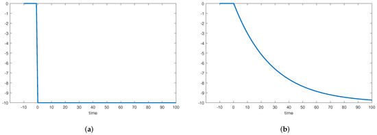
Figure 1.
The policy experiment. A permanent decrease in public investment spending at time : (a) the flow of public investment spending (), measured in percent deviations from the initial steady state; and (b) the stock of public capital (), measured in percent deviations from the initial steady state.
Figure 2 displays the macroeconomic effects of the reduction in public investment for the baseline calibration. Figure 2a shows the effects on four macroeconomic variables: labor (L; solid line), private capital (K; dashed line), output (Y; dotted line), and gross wages (w; dashed-dotted line). These four variables are key to understand the effect on the labor share of income (i.e., ), which is displayed in Figure 2b.
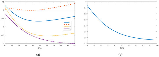
Figure 2.
The dynamic effects of a decrease in public investment spending in the baseline case of Solow-neutral public capital: (a) effects on labor employment (L), capital (K), output (Y), and the gross wage rate (w), measured in percent deviations from the initial steady state; and (b) effect on the labor share of income, measured as the percent difference to the initial steady state.
Let us start by noting in Figure 2a the continuous fall in gross wages in response to the decline in public investment. This effect simply reflects the gradual erosion of the stock of public capital, which harms the productivity of labor. Labor employment is positively affected by the public investment shock but starts falling immediately after and eventually drops below its initial level. The positive effect on labor is due to a negative wealth effect on households, who anticipate the future drop in gross and net wages (taxes also drop but not as much), whereas the subsequent decline owes to time substitution from labor to leisure due to the fall in wages. Private capital responds in a complex manner, expanding initially and in the long run, but falling somewhere during transition. These complex dynamics reflect the interplay between the direct effect of public investment (which increases the productivity of capital relative to that of labor) and the indirect effect through the decrease in labor employment (which lowers the productivity of capital). The response of output is qualitatively similar to that of labor, its main input, but quantitatively stronger due to the fall in public capital. Because the combined decline in labor employment and wages exceed that of output, the labor share of income in Figure 2b also falls over time. The impact drop in the labor share is about 0.1 percent, which increases to more than 0.6 percent in the long run.
We now turn to the alternative technological specification whereby public capital affects factor productivities. In particular, we set (so that ) and allow . We refer to this type of labor-augmenting public capital as “Harrod neutral”. Figure 3 shows the macroeconomic effects of the negative public investment shock in the case of Harrod neutrality. Despite the fact that public capital augments labor directly, the responses of labor employment and wages in Figure 3a are virtually unchanged when compared with Figure 2. The main difference lies in the response of private capital, which falls dramatically. To understand this effect, notice that, under a small (lower than one) elasticity of substitution between private capital and labor, a decrease in Harrod-neutral public capital decreases disproportionately the productivity of private capital. Hence, it is the capital factor that carries out most of the adjustment in response to the negative public investment shock. Because of the strong decline in private capital, the negative effect on output is also more pronounced in this case. As shown in Figure 3b, the response of the labor share is very different both qualitatively and quantitatively from the baseline case, being negative (i.e., below the initial value) in the first few periods after the shock, but positive (i.e., above the initial value) for the most part.
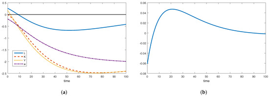
Figure 3.
The dynamic effects of a decrease in public investment spending in the alternative case of Harrod-neutral public capital: (a) effects on labor employment (L), capital (K), output (Y), and the gross wage rate (w), measured in percent deviations from the initial steady state; and (b) effect on the labor share of income, measured as the percent difference to the initial steady state.
Finally, Figure 4 shows the response of the labor share for alternative values of key parameters of the model. Figure 4a changes the leisure-labor ratio ()—which governs the labor supply elasticity—from the baseline value of 1 to the alternative values of 0.25 (inelastic supply) and 2 (elastic supply). Although the macroeconomic responses to public investment shocks are usually sensitive to this parameter [48], this is not the case with the labor share. Figure 4b varies the output elasticity of public capital () from 0.13 to 0.05 (relatively less productive public capital) and 0.20 (relatively more productive public capital). The effects on the labor share are just quantitative, with more (less) productive public capital leading to a more (less) pronounced fall in the labor share.
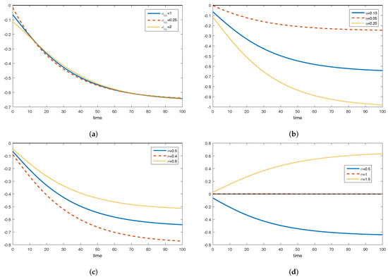
Figure 4.
Sensitivity of the dynamic response of the labor income share to alternative values of key parameters: (a) alternative values of the leisure–labor ratio (); (b) alternative values of the output elasticity of public capital (); (c) alternative values of the elasticity of substitution () (within values smaller than unity); and (d) alternative values of the elasticity of substitution () (unity and larger).
Figure 4c,d presents the sensitiveness of the labor share response to alternative values of the elasticity of substitution between private capital and labor (). Figure 4c considers small deviations of from the baseline value of 0.5 to the alternative values of 0.4 and 0.6. It shows that, although the negative response remains, the quantitative implications are rather sensitive to small changes in the elasticity of substitution between production factors: the lower the elasticity, the more pronounced the decline in the labor share. Figure 4d takes a broader perspective by comparing the baseline value of 0.5 to the values of 1 and 1.5. Not surprisingly, the labor share does not change when ; in this case, the technology is Cobb–Douglas and the income shares of both factors (private capital and labor) are fixed. However, if the elasticity of substitution is larger than unity, then the labor share increases with the public investment cut. This is because, in this case, a reduction in public capital increases the productivity of labor relative to the productivity of private capital.
6. Discussion
Our baseline results show that a permanent reduction in public investment lowers the labor share. The magnitude of this effect is not negligible: a 50% cut in public investment (e.g., from 4% to 2% of GDP), for example, would imply a decrease in the labor share of about three percent (e.g., from 66% to 63% of GDP) in the long run. These results suggest that the decline in public capital over the last decades in most of the developed world may have played an important role in the decline of the labor share of income. This is consistent with the recent empirical finding that investment in road infrastructure is positively correlated with the labor share in the Chinese manufacturing sector [15]. Our results do not imply, however, that public capital is the only, or even the most important, factor behind the decline of the labor share. Factors such as the rising levels of international trade brought about by globalization [32] or the decreasing power of labor unions [35], for instance, may have also contributed to this decline.
Two assumptions are key in our results: (1) factor-biased public capital that directly augments private capital; and (2) a lower than one elasticity of substitution between private capital and labor. Together, these assumptions imply that a public capital reduction actually increases the market value of private capital by increasing its marginal product relative to that of labor, which ultimately depresses the labor share of income. Hence, this effect operates through an increase in Tobin’s q, which is consistent with two recent findings: a rising Tobin’s q is associated with a decreased labor share [17] and the labor share decline is more pronounced in the more capital-intensive manufacturing sector [18]. If we keep the elasticity of substitution below one but instead assume that public capital directly augments labor, then a reduction in public capital mostly increases the labor share, at least in the medium and long run. Keeping public capital as capital-augmenting but allowing the substitution elasticity to be larger than unity also turns positive the labor share response. Changes in the values of other parameters affect the results only quantitatively and do not alter the main finding of this paper.
We find these assumptions plausible. The vast majority of studies that estimate the elasticity of substitution find values below unity [10,11,12,13,14]. It can actually be seen as a strength of this paper that our explanation of the decline of the labor share can, unlike other explanations, dispense with above-unity elasticities. We are not aware of any empirical evidence indicating the type of factor-augmentation induced by public capital, but biased factor-augmentation towards private capital is definitely plausible, at least for core components of public infrastructure (e.g., roads, airports, water and energy systems, etc). On the other hand, some non-core components of public investment, such as spending on R&D or spending on education and health infrastructure (e.g., schools and hospitals), are more likely to directly augment the labor factor. More research is needed to understand the factor-augmentation role of public capital.
Although it is tempting to conclude from our results that reductions in public investment imply higher income and wealth inequality, one must be cautious in establishing such generalizations. Our model emphasizes the role of factor-biased public capital in shaping the dynamics of income shares of capital and labor in a scenario of low factor substitutability. Although the distribution of income shares is related to income inequality, so is, for instance, the distribution of wages within wage earners and the distribution of wealth within capital holders. However, our model does not feature heterogeneity of capital endowments and labor productivity across households— at least for households within the same cohort—which are undeniably important for the distribution of wealth and income. For instance, using a model with capital heterogeneity, Chatterjee and Turnovsky [65] argued theoretically that public capital spending may increase wealth inequality. Turnovsky [66] also found that the implications of public infrastructure for income inequality crucially depends on whether heterogeneity of capital and productivity is taken into account. Overall, however, the available evidence seem to suggest that public investment is conducive to lower income inequality [61,62,63,73].
7. Conclusions
Income inequality has risen all over the industrialized world over the last few decades. A particular manifestation of income inequality is the well-documented decline in the share of income paid to the labor factor. Besides the obvious social concerns brought about by an unfair distribution of the economic gains, economic inequality also hinders future economic growth. To find policy solutions, understanding the causes of these inequality trends is of paramount importance.
Several explanations for the decline in the labor share have been proposed recently, often hinging on the questionable assumption that the elasticity of substitution between capital and labor is above one. This paper argues that the fall in public investment ratios and public capital stocks, which has been documented for most developed economies over the last few decades, may have contributed to the decline in the labor share. Using a small-scale macroeconomic model, we show that a permanent negative shock to public investment exerts a non-negligible negative effect on the labor share. This result requires a smaller than one elasticity of substitution and factor-biased public capital that directly augments private capital. We argue that both assumptions are practically plausible.
Public investment ratios have currently reached alarmingly low levels. International organizations such as the Organization for Economic Cooperation and Development [74] and the IMF [16] have warned that a widening “infrastructure gap” is likely to restrain sustainable long-run growth. Our results suggest that these low levels of public investment spending are also likely to contribute to income inequality via a smaller share of income devoted to the labor factor. Increasing the share of income devoted to public investment could thus boost not only economic efficiency but also economic equity. On the efficiency side, the spillover effects of public investment enhance total factor productivity and promote long-run growth [75]. Given the current infrastructure gap, these productivity gains could be substantial. On the equity side, a larger public investment ratio would not only contribute to a large share of income received by wage earners, but also improve social cohesion through more and better social infrastructure. A study by Dercon [76], for instance, shows how fundamental public infrastructure can be to move households out of poverty.
As with all studies, however, this one has limitations, which motivate future research. Perhaps the major limitation of the present study is the neglect of agent heterogeneity in terms of labor productivity and capital endowments. In our model, financial wealth varies between but not within generations, whereas labor productivity does not vary at all. While this allows focusing directly on factor shares of income, it precludes more general considerations about the effects of public investment on income and wealth inequality. We therefore believe that one fruitful avenue of research would be to study the role of public investment to income inequality in an extended model of factor-biased public capital with heterogeneous agents. Another promising line of research would be to simulate/estimate the “inequality multiplier” of public investment, broken down by investment type, which would inform the government about the types of public investment that are more or less conducive to economic equity. We intend to pursue these lines of research in the future.
Supplementary Materials
The following are available online at http://www.mdpi.com/2071-1050/10/11/3895/s1, Technical Appendix.
Author Contributions
Conceptualization, P.R.D.B. and A.G.; Methodology, P.R.D.B.; Software, P.R.D.B.; Formal Analysis, P.R.D.B.; Investigation, P.R.D.B.; Writing—Original Draft Preparation, P.R.D.B. and A.G.; Writing—Review and Editing, P.R.D.B. and A.G.; and Funding Acquisition, A.G.
Funding
This research was funded by University–Company call of the Basque Government, project number UE2016-10.
Conflicts of Interest
The authors declare no conflict of interest.
References
- IMF. Fostering Inclusive Growth; Staff Note Prepared for G-20 Leaders’ Summit, Hamburg, Germany, 7–8 July 2017; International Monetary Fund: Washington, DC, USA, 2017. [Google Scholar]
- UNDP. UNDP’s Strategy for Inclusive and Sustainable Growth; United Nations Development Programme: New York, NY, USA, 2017. [Google Scholar]
- World Bank. World Development Report 2017: Governance and the Law; International Bank for Reconstruction and Development, The World Bank: Washington, DC, USA, 2017. [Google Scholar]
- Ostry, J.D.; Berg, A.; Tsangarides, C.G. Redistribution, Inequality, and Growth; IMF Staff Discussion Note 14/02; International Monetary Fund: Washington, DC, USA, 2014. [Google Scholar]
- Piketty, T. Capital in the Twenty-First Century; Harvard University Press: Cambridge, MA, USA, 2017; ISBN 978-0-674-43000-6. [Google Scholar]
- Piketty, T.; Saez, E. Inequality in the long run. Science 2014, 344, 838–843. [Google Scholar] [CrossRef] [PubMed]
- Dao, M.C.; Das, M.; Koczan, Z.; Weicheng, L. Understanding the downward trend in labor income shares. In World Economic Outlook: Gaining Momentum? International Monetary Fund: Washington, DC, USA, 2017; pp. 121–172. ISBN 978-1-47559-214-6. [Google Scholar]
- Karabarbounis, L.; Neiman, B. The global decline of the labor share. Q. J. Econ. 2014, 129, 61–103. [Google Scholar] [CrossRef]
- Villar-Rodriguez, E.; Osaba-Icedo, E.; Del-Ser-Lorente, J. Quantum computing: Six key factors to understand the future of computation. DYNA 2018, 93, 238–341. [Google Scholar] [CrossRef]
- Chirinko, R.S. σ: The long and short of it. J. Macroecon. 2008, 30, 671–686. [Google Scholar] [CrossRef]
- Young, A.T.U.S. elasticities of substitution and factor augmentation at the industry level. Macroecon. Dyn. 2013, 17, 861–897. [Google Scholar] [CrossRef]
- Herrendorf, B.; Herrington, C.; Valentinyi, A. Sectoral technology and structural transformation. Am. Econ. J. Macroecon. 2015, 7, 104–133. [Google Scholar] [CrossRef]
- León-Ledesma, M.A.; McAdam, P.; Willman, A. Production technology estimates and balanced growth. Oxf. Bull. Econ. Stat. 2015, 77, 40–65. [Google Scholar] [CrossRef]
- Chirinko, R.S.; Mallick, D. The substitution elasticity, factor shares, and the low-frequency panel model. Am. Econ. J. Macroecon. 2017, 9, 225–253. [Google Scholar] [CrossRef]
- Zhang, X.; Wan, G.; Wang, X. Road infrastructure and the share of labor income: Evidence from China’s manufacturing sector. Econ. Syst. 2017, 41, 513–523. [Google Scholar] [CrossRef]
- Abiad, A.; Almansour, A.; Furceri, D.; Mulas-Granados, C.; Topalova, P. Is it time for an infrastructure push? The macroeconomic effects of public investment. In World Economic Outlook: Legacies, Clouds, Uncertainties; International Monetary Fund: Washington, DC, USA, 2014; pp. 1–40. ISBN 978-1-48438-0-666. [Google Scholar]
- Gonzalez, I.; Trivín, P. Finance and the global decline of the labour share. Int. Lab. Organ. 2016, 43, 17–68. [Google Scholar]
- Alvarez-Cuadrado, F.; Van Long, N.; Poschke, M. Capital-labor substitution, structural change and the labor income share. J. Econ. Dyn. Control 2018, 87, 206–231. [Google Scholar] [CrossRef]
- Stanton, E.A. The tragedy of maldistribution: Climate, sustainability, and equity. Sustainability 2012, 4, 394–411. [Google Scholar] [CrossRef]
- Rogers, S.H.; Gardner, K.H.; Carlson, C.H. Social capital and walkability as social aspects of sustainability. Sustainability 2013, 5, 3473–3483. [Google Scholar] [CrossRef]
- Tirado, A.A.; Morales, M.R.; Lobato-Calleros, O. Additional indicators to promote social sustainability within government programs: equity and efficiency. Sustainability 2015, 7, 9251–9267. [Google Scholar] [CrossRef]
- Socol, C.; Marinas, M.; Socol, A.G.; Armeanu, D. Fiscal adjustment programs versus socially sustainable competitiveness in EU countries. Sustainability 2018, 10, 3390. [Google Scholar] [CrossRef]
- Lotero, L.; Hurtado, R.G.; Floría, L.M.; Gómez-Gardeñes, J. Rich do not rise early: Spatio-temporal patterns in the mobility networks of different socio-economic classes. R. Soc. Open Sci. 2016, 3, 150654. [Google Scholar] [CrossRef] [PubMed]
- Sen, A. On Economic Inequality; Clarendon Press: Oxford, UK, 1973; ISBN 978-01-98-28193-1. [Google Scholar]
- Aghion, P.; Williamson, J.G. Growth, Inequality, and Globalization: Theory, History, and Policy; Cambridge University Press: Cambridge, UK, 1998; ISBN 978-05-21-65910-9. [Google Scholar]
- Keister, L.A. Wealth in America: Trends in Wealth Inequality; Cambridge University Press: Cambridge, UK, 2000; ISBN 978-05-21-62751-1. [Google Scholar]
- Piketty, T.; Saez, E. Income inequality in the United States, 1913–1998. Q. J. Econ. 2003, 118, 1–39. [Google Scholar] [CrossRef]
- Piketty, T.; Zucman, G. Wealth and inheritance in the long run. In Handbook of Income Distribution; Atkinson, A.B., Bourguignon, F., Eds.; Elsevier B.V.: Amsterdam, The Netherlands, 2015; ISBN 978-0-444-59430-3. [Google Scholar]
- Cagetti, M.; De Nardi, M. Wealth inequality: Data and models. Macroecon. Dyn. 2008, 12, 285–313. [Google Scholar] [CrossRef]
- Benhabib, J.; Bisin, A.; Zhu, S. The distribution of wealth and fiscal policy in economies with finitely lived agents. Econometrica 2011, 79, 123–157. [Google Scholar] [CrossRef]
- Berman, Y.; Ben-Jacob, E.; Shapira, Y. The dynamics of wealth inequality and the effect of income distribution. PLoS ONE 2016, 11, e0154196. [Google Scholar] [CrossRef] [PubMed]
- Harrison, A.E. Has Globalization Eroded Labor’s Share? Some Cross-Country Evidence; University of California at Berkeley and NBER: Berkeley, CA, USA, 2002. [Google Scholar]
- Autor, D.; Dorn, D.; Katz, L.F.; Patterson, C.; Van Reenen, J. The Fall of the Labor Share and the Rise of Superstar Firms; IZA DP No. 10756; IZA Institute of Labor Economics: Bonn, Germany, 2017. [Google Scholar]
- Fichtenbaum, R. The impact of unions on labor’s share of income: A time-series analysis. Rev. Polit. Econ. 2009, 21, 567–588. [Google Scholar] [CrossRef]
- Abdih, Y.; Danninger, S. What Explains the Decline of the U.S. Labor Share of Income? An Analysis of State and Industry Level Data; IMF Working Paper WP/17/167; International Monetary Fund: Washington, DC, USA, 2017. [Google Scholar]
- Aschauer, D. Is public expenditure productive? J. Monet. Econ. 1980, 23, 177–200. [Google Scholar] [CrossRef]
- Evans, P.; Karras, G. Is government capital productive? Evidence from a panel of seven countries. J. Macroecon. 1994, 16, 271–279. [Google Scholar] [CrossRef]
- Holtz-Eakin, D. Public-sector capital and the productivity puzzle. Rev. Econ. Stat. 1994, 76, 12–21. [Google Scholar] [CrossRef]
- Rokicki, B.; Stępniak, M. Major transport infrastructure investment and regional economic development—An accessibility-based approach. J. Transp. Geogr. 2018, 72, 36–49. [Google Scholar] [CrossRef]
- Munnell, A.H. Policy watch: Infrastructure investment and economic growth. J. Econ. Perspect. 1992, 6, 189–198. [Google Scholar] [CrossRef]
- Pereira, A.M.; Andraz, J.M. Public highway spending and state spillovers in the USA. Appl. Econ. Lett. 2004, 11, 785–788. [Google Scholar] [CrossRef]
- Romp, W.; de Haan, J. Public capital and economic growth: A critical survey. Perspektiven der Wirtschaftspolitik 2007, 8, 6–52. [Google Scholar] [CrossRef]
- Bom, P.R.D.; Ligthart, J.E. What have we learned from three decades of research on the productivity of public capital? J. Econ. Surv. 2014, 28, 889–916. [Google Scholar] [CrossRef]
- Facchini, F.; Seghezza, E. Public spending structure, minimal state and economic growth in France (1870–2010). Econ. Model. 2018, 72, 151–164. [Google Scholar] [CrossRef]
- Gherghina, S.C.; Onofrei, M.; Vintilă, G.; Armeanu, D.S. Empirical evidence from EU-28 countries on resilient transport infrastructure systems and sustainable economic growth. Sustainability 2018, 10, 2900. [Google Scholar] [CrossRef]
- Baxter, M.; King, R.G. Fiscal Policy in General Equilibrium. Am. Econ. Rev. 1993, 83, 315–334. [Google Scholar]
- Turnovsky, S.J.; Fisher, W.H. The composition of government expenditure and its consequences for macroeconomic performance. J. Econ. Dyn. Control 1995, 19, 747–786. [Google Scholar] [CrossRef]
- Bom, P.R.D.; Ligthart, J.E. Public infrastructure investment, output dynamics, and balanced budget fiscal rules. J. Econ. Dyn. Control 2014, 40, 334–354. [Google Scholar] [CrossRef]
- Leeper, E.R.; Walker, T.B.; Yang, S.-C. Government investment and fiscal stimulus. J. Monet. Econ. 2010, 57, 1000–1012. [Google Scholar] [CrossRef]
- Bouakez, H.; Guillard, M.; Roulleau-Pasdeloup, J. Public investment, time to build, and the zero lower bound. Rev. Econ. Dyn. 2017, 23, 60–79. [Google Scholar] [CrossRef]
- Barro, R.J. Government spending in a simple model of endogeneous growth. J. Polit. Econ. 1990, 98, S103–S125. [Google Scholar] [CrossRef]
- Fisher, W.H.; Turnovsky, S.J. Public Investment, congestion, and private capital accumulation. Econ. J. 1998, 108, 399–413. [Google Scholar] [CrossRef]
- Bom, P.R.D. Factor-biased public capital and private capital crowding out. J. Macroecon. 2017, 52, 100–117. [Google Scholar] [CrossRef]
- Dreger, C.; Reimers, H.-E. Does public investment stimulate private investment? Evidence for the euro area. Econ. Model. 2016, 58, 154–158. [Google Scholar] [CrossRef]
- Eden, M.; Kraay, A. “Crowding in” and the Returns to Government Investment in Low-Income Countries; Policy Research Working Paper No. 6781; The World Bank: Washington, DC, USA, 2014. [Google Scholar]
- Afonso, A.; St. Aubyn, M. Macroeconomic rates of return of public and private investment: Crowding-in and crowding-out effects. Manch. Sch. 2009, 77, 21–39. [Google Scholar] [CrossRef]
- Cavallo, E.; Daude, C. Public investment in developing countries: A blessing or a curse? J. Comp. Econ. 2011, 39, 61–85. [Google Scholar] [CrossRef]
- Chatterjee, S.; Gibson, J.; Rioja, F. Public investment, debt, and welfare: A quantitative analysis. J. Macroecon. 2018, 56, 204–217. [Google Scholar] [CrossRef]
- Heijdra, B.J.; Meijdam, L. Public investment and intergenerational distribution. J. Econ. Dyn. Control 2002, 26, 707–735. [Google Scholar] [CrossRef]
- Bom, P.R.D. Fiscal rules and the intergenerational welfare effects of public investment. Econ. Model. 2018, in press. [Google Scholar] [CrossRef]
- Lopez, H. Macroeconomics and Inequality; The World Bank Research Workshop, Macroeconomic Challenges in Low Income Countries; The World Bank: Washington, DC, USA, 2003. [Google Scholar]
- Calderón, C.; Chong, A. Volume and quality of infrastructure and the distribution of income: An empirical investigation. Rev. Income Wealth 2004, 50, 87–106. [Google Scholar] [CrossRef]
- Calderón, C.; Servén, L. The Effects of Infrastructure Development on Growth and Income Distribution; Policy Research Working Paper No. 3400; The World Bank: Washington, DC, USA, 2004. [Google Scholar]
- Banerjee, A.; Duflo, E.; Qian, N. On the Road: Access to Transportation Infrastructure and Economic Growth in China; NBER Working Paper No. 17897; NBER: Cambridge, MA, USA, 2012. [Google Scholar]
- Chatterjee, S.; Turnovsky, S.J. Infrastructure and inequality. Eur. Econ. Rev. 2012, 56, 1730–1745. [Google Scholar] [CrossRef]
- Turnovsky, S.J. Economic growth and inequality: The role of public investment. J. Econ. Dyn. Control 2015, 61, 204–221. [Google Scholar] [CrossRef]
- Blanchard, O.J. Debt, deficits, and finite horizons. J. Polit. Econ. 1985, 93, 223–247. [Google Scholar] [CrossRef]
- Yaari, M.E. Uncertain lifetime, life insurance, and the theory of the consumer. Rev. Econ. Stud. 1965, 32, 137–150. [Google Scholar] [CrossRef]
- Schmitt-Grohé, S.; Uribe, M. Closing small open economy models. J. Int. Econ. 2003, 61, 163–185. [Google Scholar] [CrossRef]
- AMECO Database. Available online: https://ec.europa.eu/info/business-economy-euro/indicators-statistics/economic-databases/macro-economic-database-ameco/ameco-database_en (accessed on 8 March 2016).
- Investment and Capital Stock (ICSD). Available online: https://data.world/imf/investment-and-capitalstock-i (accessed on 8 March 2016).
- Drautzburg, T.; Uhlig, H. Fiscal stimulus and distortionary taxation. Rev. Econ. Dyn. 2015, 18, 894–920. [Google Scholar] [CrossRef]
- Calderón, C.; Servén, L. Infrastructure, Growth, and Inequality: An Overview; Policy Research Working Paper No. 7034; The World Bank: Washington, DC, USA, 2014. [Google Scholar]
- OECD. Strategic Transport Infrastructure Needs to 2030; OECD Publishing: Paris, France, 2012; ISBN 978-92-64-16862-6. [Google Scholar]
- ILO. Reducing Decent Work Deficits in Periods of Low Growth; What Works Research Brief No. 6; International Labour Organization: Geneva, Switzerland, 2017. [Google Scholar]
- Dercon, S. Risk, poverty and vulnerability in Africa. J. Afr. Econ. 2005, 14, 483–488. [Google Scholar] [CrossRef]
© 2018 by the authors. Licensee MDPI, Basel, Switzerland. This article is an open access article distributed under the terms and conditions of the Creative Commons Attribution (CC BY) license (http://creativecommons.org/licenses/by/4.0/).