Deep Decarbonisation from a Biophysical Perspective: GHG Emissions of a Renewable Electricity Transformation in the EU


Abstract
1. Introduction
2. Background
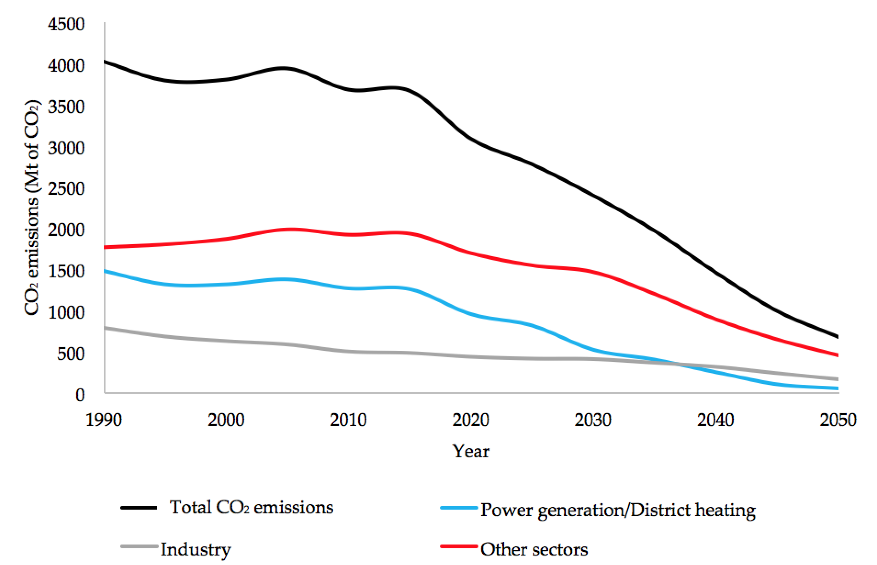
2.1. Decarbonisation in EU Policy
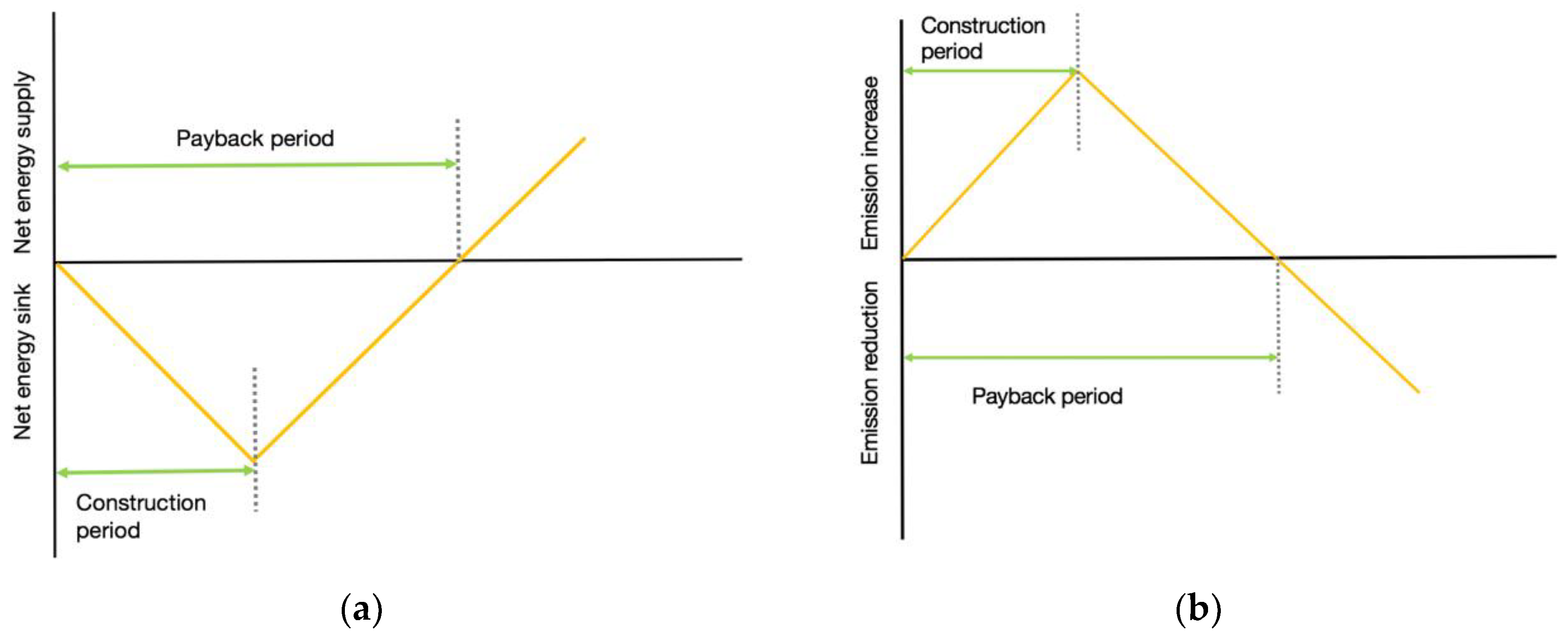
2.2. Energy and GHG Payback Time
3. Alternative Decarbonisation Pathways
3.1. Modelling Assumptions
3.1.1. Grid Flexibility
3.1.2. GHG Emissions of Renewable Infrastructure, Storage and Fossil Plants
3.2. Modelling Equations
- GHG_stn are the GHG emissions, in tons of CO2 equivalent, emitted at year n due to the cultivation, fabrication and construction (CFC) of infrastructure;
- GWPV and GWwind are the amounts of extra solar PV and wind power capacity installed each year;
- GWhPHS and GWhBES are the amounts of extra storage capacity, PHS and BES, added each year;
- GHG_opn are the varying infrastructure emissions at each year n, depending, in turn, on the electricity mix and expressed in tons of CO2 equivalent/GW for renewable infrastructure and tons of CO2 equivalent/GWh for renewable infrastructure;
- GWhn is the electricity generation at year n by each technology.
4. Results and Discussion
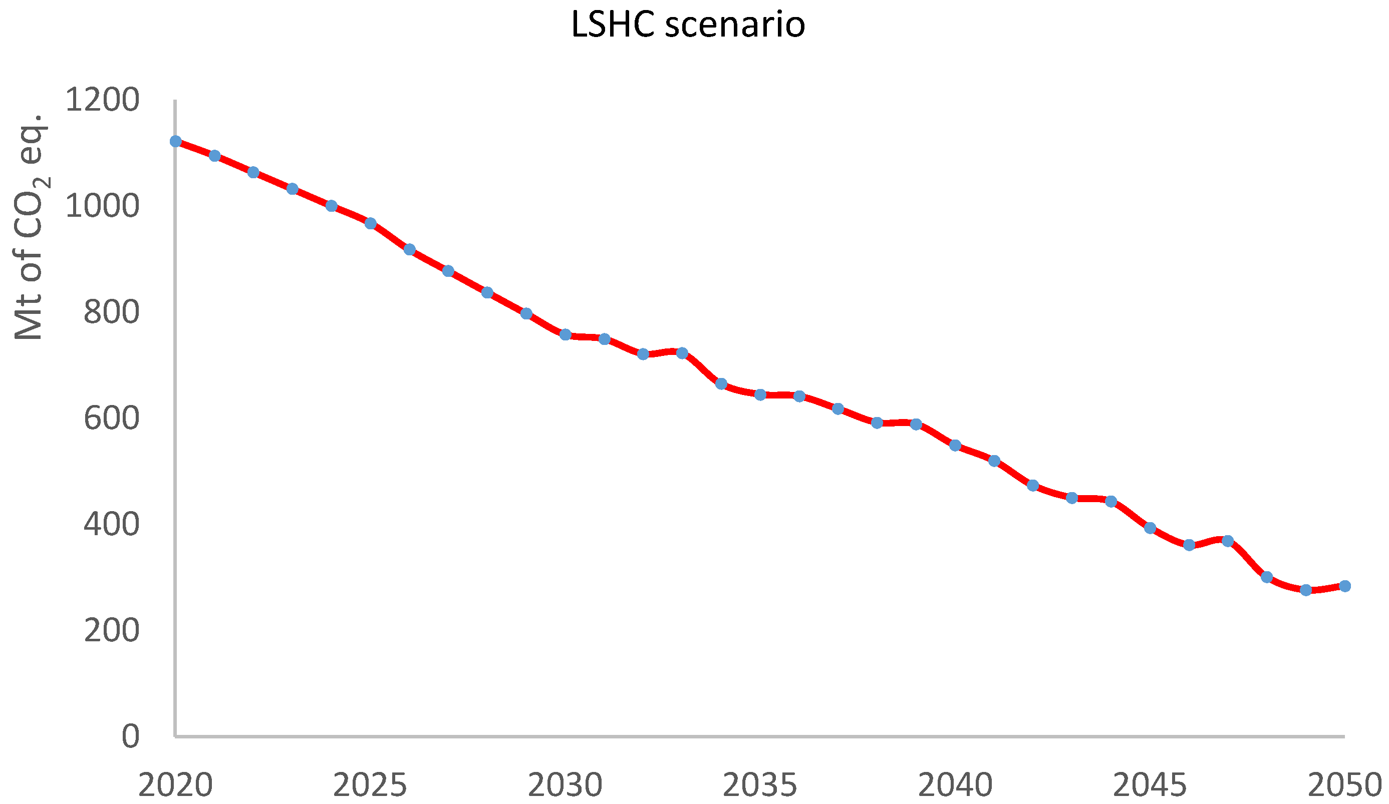
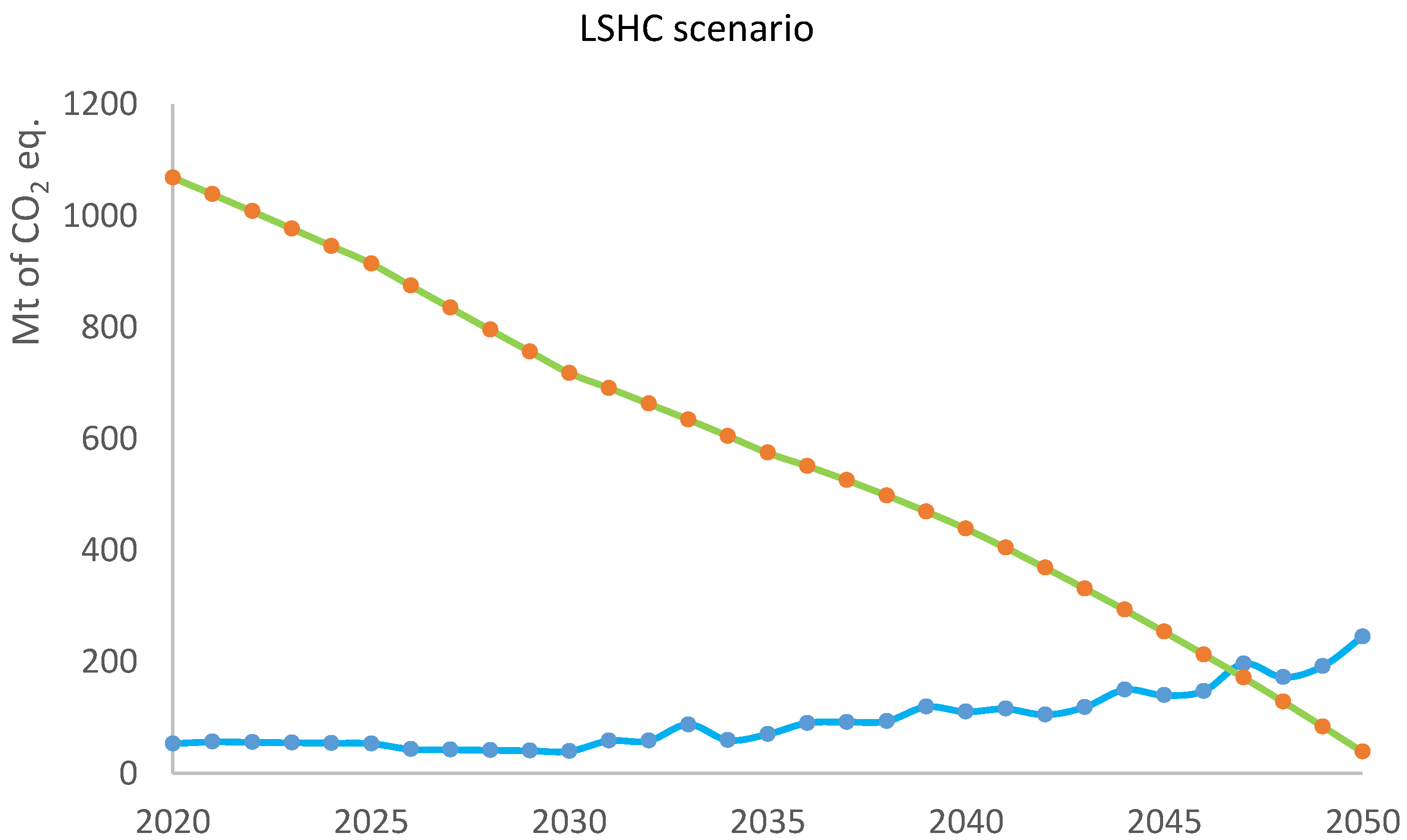
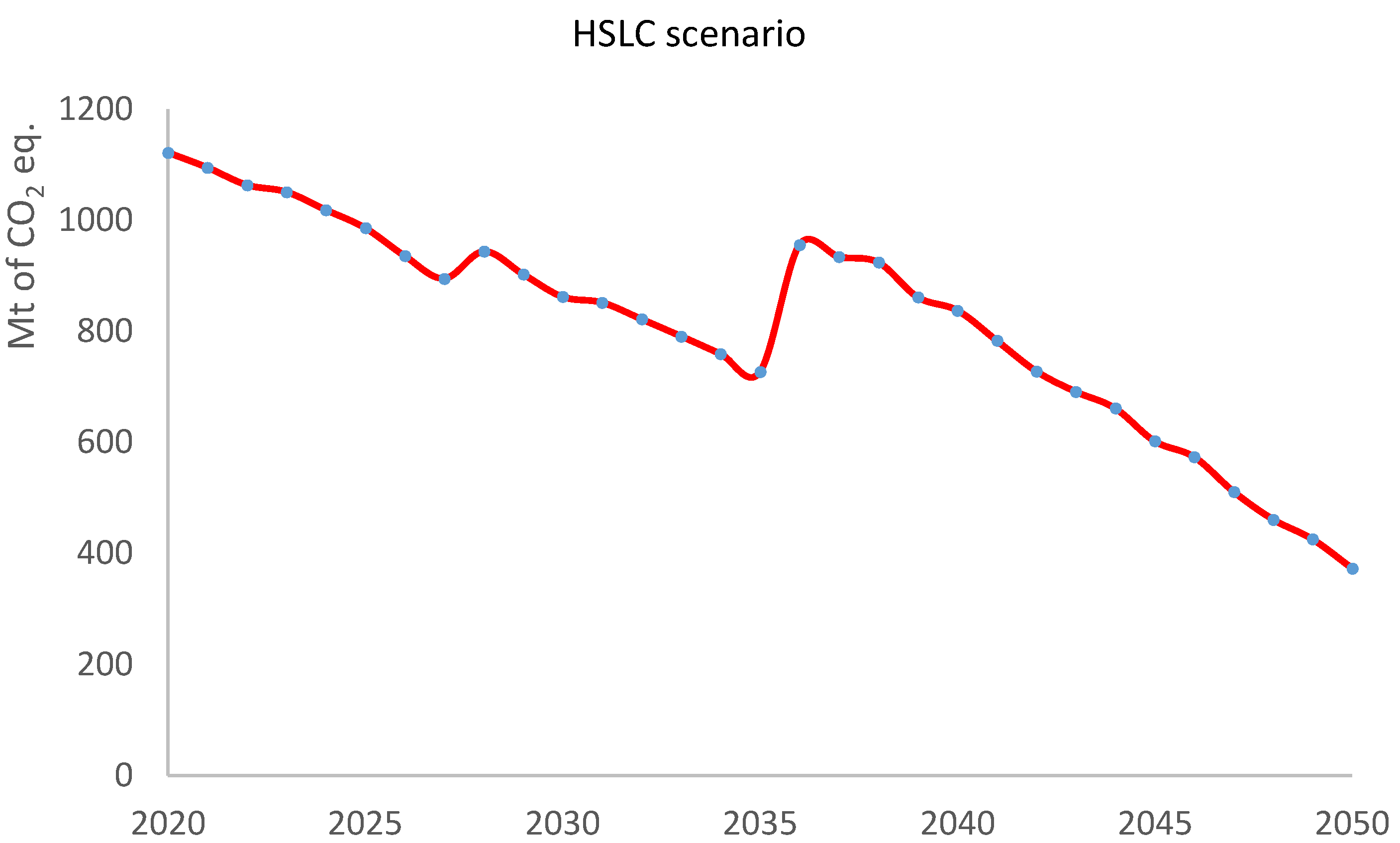
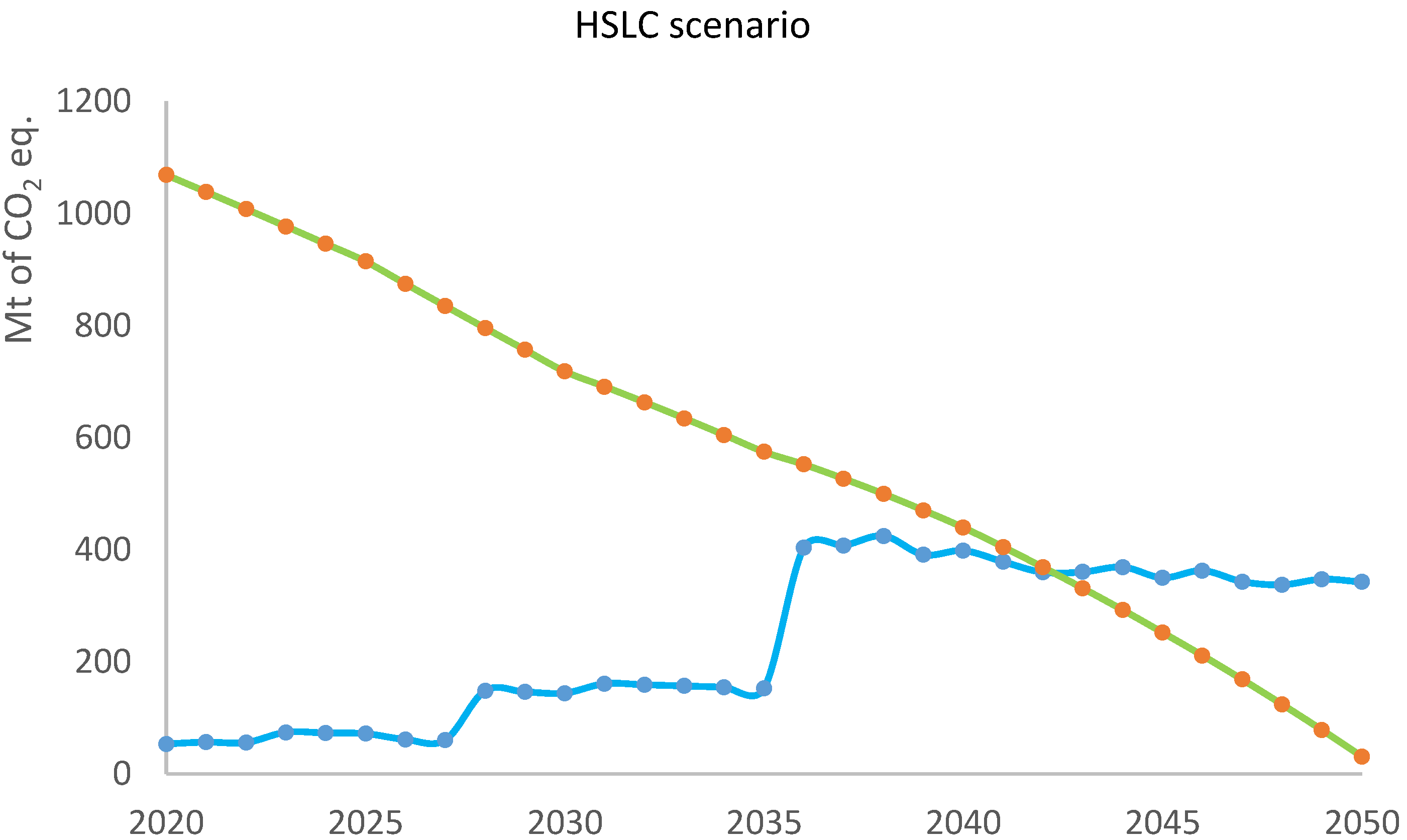
4.1. GHG Emission Curves and Cumulative Emissions
- Emission curves at a yearly resolution, useful to comment on the temporal behaviour of emissions and their possible non-linear evolution;
- Cumulative emissions up to the year 2050, i.e., the sum of the yearly emissions, which can be related to carbon budgets;
- Yearly emissions at the target year 2050, currently the only view used to inform EU decision-making processes (with different targets set for different years).
4.2. Analysis of Variational Ranges in the Results
4.3. Discussion
5. Conclusions
Author Contributions
Funding
Acknowledgments
Conflicts of Interest
References
- Smil, V. Energy Transitions: History, Requirements, Prospects; Praeger: Santa Barbara, CA, USA, 2010; ISBN 9780313381775. [Google Scholar]
- Cottrell, F. Energy and Society: The Relation between Energy, Social Changes, and Economic Development; McGraw-Hill: New York, NY, USA, 1955. [Google Scholar]
- Giampietro, M.; Mayumi, K.; Sorman, A. The Metabolic Pattern of Societies: Where Economists Fall Short; Routledge: London, UK, 2011. [Google Scholar]
- European Commission. European Energy Security Strategy; European Commission: Brussels, Belgium, 2014. [Google Scholar]
- Vahtra, P. Energy security in Europe in the aftermath of 2009 Russia-Ukraine gas crisis. In EU-Russia Gas Connection: Pipes, Politics and Problems; Pan European Institute: Turku, Finland, 2009; pp. 159–165. [Google Scholar]
- European Commission. Proposal for a Directive of the European Parliament and of the Council on the Promotion of the Use of Energy from Renewable Sources (Recast); European Commission: Brussels, Belgium, 2017; Volume 0382 (COD), pp. 1–116. [Google Scholar]
- Scholz, R.; Beckmann, M.; Pieper, C.; Muster, M.; Weber, R. Considerations on providing the energy needs using exclusively renewable sources: Energiewende in Germany. Renew. Sustain. Energy Rev. 2014, 35, 109–125. [Google Scholar] [CrossRef]
- Georgescu-Roegen, N. The Entropy Law and the Economic Process; Harvard University Press: Boston, MA, USA, 1971. [Google Scholar]
- Giampietro, M.; Mayumi, K.; Ramos-Martin, J. Multi-scale integrated analysis of societal and ecosystem metabolism (MuSIASEM): Theoretical concepts and basic rationale. Energy 2009, 34, 313–322. [Google Scholar] [CrossRef]
- European Commission. Energy Roadmap 2050; European Commission: Brussels, Belgium, 2012. [Google Scholar]
- European Commission. EU Reference Scenario 2016: Energy, Transport and GHG Emissions Trends to 2050; European Commission: Brussels, Belgium, 2016; ISBN 978-92-79-52373-1. [Google Scholar]
- Kondziella, H.; Bruckner, T. Flexibility requirements of renewable energy based electricity systems—A review of research results and methodologies. Renew. Sustain. Energy Rev. 2016, 53, 10–22. [Google Scholar] [CrossRef]
- Eurostat. Greenhouse Gas Emission Statistics—Emission Inventories; Eurostat: Luxembourg, 2018. [Google Scholar]
- 2050 Low-Carbon Economy|Climate Action. Available online: https://ec.europa.eu/clima/policies/strategies/2050_en (accessed on 26 March 2018).
- European Commission. European Council Conclusions on Jobs, Growth and Competitiveness, as Well as Some of the Other Items (Paris Agreement and Digital Europe); European Commission: Brussels, Belgium, 2018. [Google Scholar]
- European Commission. Clean Energy for All Europeans. In Communication from Commission to European Parliament Council European Economy Society Committee of Committee Regions; European Commission: Brussels, Belgium, 2016; Volume COM (2016). [Google Scholar]
- Bruckner, T.; Bashmakov, I.A.; Mulugetta, Y.; Chum, H.; De la Vega Navarro, A.; Edmonds, J.; Faaij, A.; Fungtammasan, B.; Garg, A.; Hertwich, E.; et al. In Proceedings of the Energy systems. Climate Change 2014 Mitigation Climate Change Contrib. Work Group III to Fifth Assessment Rep. Intergovernmental Panel Climate Change, Copenhagen, Denmark, 1 November 2014. [Google Scholar]
- European Commission. Modelling Tools for EU Analysis. Available online: https://ec.europa.eu/clima/policies/strategies/analysis/models_en (accessed on 7 February 2018).
- Steinke, F.; Wolfrum, P.; Hoffmann, C. Grid vs. storage in a 100% renewable Europe. Renew. Energy 2013, 50, 826–832. [Google Scholar] [CrossRef]
- Esteban, M.; Zhang, Q.; Utama, A. Estimation of the energy storage requirement of a future 100% renewable energy system in Japan. Energy Policy 2012, 47, 22–31. [Google Scholar] [CrossRef]
- Denholm, P.; Hand, M. Grid flexibility and storage required to achieve very high penetration of variable renewable electricity. Energy Policy 2011, 39, 1817–1830. [Google Scholar] [CrossRef]
- Denholm, P.; Margolis, R. Energy Storage Requirements for Achieving 50% Solar Photovoltaic Energy Penetration in California; National Renewable Energy Laboratory: Golden, CO, USA, 2016. [Google Scholar]
- Murphy, D.J.; Hall, C.A.S. Energy return on investment, peak oil, and the end of economic growth. Ann. N. Y. Acad. Sci. 2011, 1219, 52–72. [Google Scholar] [CrossRef] [PubMed]
- Court, V.; Fizaine, F. Long-Term Estimates of the Energy-Return-on-Investment (EROI) of Coal, Oil, and Gas Global Productions. Ecol. Econ. 2017, 138, 145–159. [Google Scholar] [CrossRef]
- Giampietro, M.; Mayumi, K.; Ramos-Martin, J. Can Biofuels Replace Fossil Energy Fuels? A Multi-Scale Integrated Analysis Based on the Concept of Societal and Ecosystem Metabolism: Part 1. Int. J. Transdiscip. Res. 2006, 1, 51–87. [Google Scholar]
- Mann, S.; de Wild, M.J. The energy payback time of advanced crystalline silicon PV modules in 2020: A prospective study. Prog. Photovolt. 2014, 22, 1180–1194. [Google Scholar] [CrossRef]
- Fthenakis, V.; Alsema, E. Photovoltaics energy payback times, greenhouse gas emissions and external costs: 2004–early 2005 status. Prog. Photovolt. Res. Appl. 2006, 14, 275–280. [Google Scholar] [CrossRef]
- Gibbs, H.K.; Johnston, M.; Foley, J.A.; Holloway, T.; Monfreda, C.; Ramankutty, N.; Zaks, D. Carbon payback times for crop-based biofuel expansion in the tropics: The effects of changing yield and technology. Environ. Res. Lett. 2008, 3, 034001. [Google Scholar] [CrossRef]
- Mello, F.; Cerri, C.; Davies, C. Payback time for soil carbon and sugar-cane ethanol. Nat. Clim. Chang. 2014, 4, 605–609. [Google Scholar] [CrossRef]
- Barnhart, C.J.; Benson, S.M. On the importance of reducing the energetic and material demands of electrical energy storage. Energy Environ. Sci. 2013, 6, 1083. [Google Scholar] [CrossRef]
- Denholm, P.; Ela, E.; Kirby, B.; Milligan, M. The Role of Energy Storage with Renewable Electricity Generation; National Renewable Energy Laboratory: Golden, CO, USA, 2010; pp. 1–53. [Google Scholar]
- Nugent, D.; Sovacool, B.K. Assessing the lifecycle greenhouse gas emissions from solar PV and wind energy: A critical meta-survey. Energy Policy 2014, 65, 229–244. [Google Scholar] [CrossRef]
- Cilliers, P. Complexity and Postmodernism: Understanding Complex Systems; Taylor & Francis: Abingdon-on-Thames, UK, 2002. [Google Scholar]
- European Commission. Energy Modelling. Available online: https://ec.europa.eu/energy/en/data-analysis/energy-modelling (accessed on 22 July 2018).
- Renner, A.; Giampietro, M. The Regulation of Alternatives in the Electric Grid: Nice Try Guys, But Let’s Move On. In International Conference on Sustainable Energy and Environment Sensing (SEES); University of Cambridge: Cambridge, UK, 2018. [Google Scholar]
- Kuhn, P. Iteratives Modell zur Optimierung von Speicherausbau und-Betrieb in Einem Stromsystem mit Zunehmend Fluktuierender Erzeugung; University of Munchen: Munchen, Germany, 2012. [Google Scholar]
- Kougias, I.; Szabó, S. Pumped hydroelectric storage utilization assessment: Forerunner of renewable energy integration or Trojan horse? Energy 2017, 140, 318–329. [Google Scholar] [CrossRef]
- Gimeno-Gutiérrez, M.; Lacal-Arántegui, R. Assessment of the European Potential for Pumped Hydropower Energy Storage: A GIS-Based Assessment of Pumped Hydropower Storage Potential; European Commission: Brussels, Belgium, 2013; ISBN 9789279295119. [Google Scholar]
- Denholm, P.; Kulcinski, G.L. Life cycle energy requirements and greenhouse gas emissions from large scale energy storage systems. Energy Convers. Manag. 2004, 45, 2153–2172. [Google Scholar] [CrossRef]
- Romare, M.; Dahllöf, L. The Life Cycle Energy Consumption and Greenhouse Gas Emissions from Lithium-Ion Batteries a Study with Focus on Current Technology and Batteries for Light-Duty Vehicles; Swedish Environmental Research Institute: Stockholm, Sweden, 2017. [Google Scholar]
- Moro, A.; Lonza, L. Electricity carbon intensity in European Member States: Impacts on GHG emissions of electric vehicles. Transp. Res. Part D Transp. Environ. 2017. [Google Scholar] [CrossRef]
- Guezuraga, B.; Zauner, R.; Pölz, W. Life cycle assessment of two different 2 MW class wind turbines. Renew. Energy 2012, 37, 37–44. [Google Scholar] [CrossRef]
- Oebels, K.B.; Pacca, S. Life cycle assessment of an onshore wind farm located at the northeastern coast of Brazil. Renew. Energy 2013, 53, 60–70. [Google Scholar] [CrossRef]
- Pehnt, M. Dynamic life cycle assessment (LCA) of renewable energy technologies. Renew. Energy 2006, 31, 55–71. [Google Scholar] [CrossRef]
- Reich, N.H.; Alsema, E.A.; van Sark, W.G.J.; Turkenburg, W.C.; Sinke, W.C. Greenhouse gas emissions associated with photovoltaic electricity from crystalline silicon modules under various energy supply options. Prog. Photovolt. Res. Appl. 2011, 19, 603–613. [Google Scholar] [CrossRef]
- Meyer-Ohlendorf, N.; Voß, P.; Velten, E.; Görlach, B. EU Greenhouse Gas Emission Budget: Implications for EU Climate Policies; European Commission: Brussels, Belgium, 2018. [Google Scholar]
- Aneke, M.; Wang, M. Energy storage technologies and real life applications—A state of the art review. Appl. Energy 2016, 179, 350–377. [Google Scholar] [CrossRef]
- Jackson, T. Negotiating Sustainable Consumption: A Review of the Consumption Debate and its Policy Implications. Energy Environ. 2004, 15, 1027–1051. [Google Scholar] [CrossRef]
- Sorman, A.H. Metabolism, Societal. In Degrowth: A Vocabulary for a New Era; Routledge: London, UK, 2014; Volume 160. [Google Scholar]


| Variable | 2020 | 2030 | 2040 | 2050 |
|---|---|---|---|---|
| Gross electricity consumption (GWh) | 3,665,400 | 3,666,000 | 4,357,600 | 5,140,600 |
| Daily electricity consumption (GWh) | 10,042 | 10,043 | 11,939 | 14,084 |
| Hydropower (%) | 10 | 10 | 9 | 7 |
| Nuclear (%) | 24 | 16 | 8 | 3 |
| Fossil plants (%) | 40 | 27 | 14 | 0 |
| Wind power (%) | 14 | 29 | 46 | 62 |
| Solar power (%) | 6 | 12 | 20 | 27 |
| Other renewables (%) | 5 | 5 | 5 | 0 |
| Variable | Alternative Pathway | 2020 | 2030 | 2040 | 2050 |
|---|---|---|---|---|---|
| Gross electricity consumption (GWh) | LSHC | 3,665,400 | 3,666,000 | 4,357,600 | 5,140,600 |
| HSLC | 3,665,400 | 3,666,000 | 4,357,600 | 5,140,600 | |
| Gross production from wind power (GWh) | LSHC | 505,270 | 1,057,690 | 2,228,440 | 5,110,500 |
| HSLC | 505,270 | 1,057,690 | 2,049,370 | 3,194,070 | |
| Gross production from solar PV (GWh) | LSHC | 216,540 | 453,300 | 955,040 | 2,190,220 |
| HSLC | 216,540 | 453,300 | 878,300 | 1,587,910 | |
| Curtailment rate (%) | LSHC | 0 | 0 | 10 | 60 |
| HSLC | 0 | 0 | 0 | 20 | |
| Storage capacity (GWh) | LSHC | 600 | 600 | 600 | 600 |
| HSLC | 600 | 14,570 | 51,100 | 87,630 | |
| Wind power UF (%) | LSHC | 24 | 24 | 21 | 15 |
| HSLC | 24 | 24 | 23 | 21 | |
| Solar PV UF (%) | LSHC | 13 | 13 | 12 | 8 |
| HSLC | 13 | 13 | 13 | 11 | |
| Wind power capacity (GW) | LSHC | 240 | 500 | 1060 | 2430 |
| HSLC | 240 | 500 | 980 | 1760 | |
| Solar PV capacity (GW) | LSHC | 190 | 400 | 840 | 1920 |
| HSLC | 190 | 400 | 770 | 1390 |
| (a) | ||
| Variable | Wind Power | Solar PV |
| Number of studies | 41 | 23 |
| Hub height (m) | 10–108 | N/A |
| Rotor diameter (m) | 2–116 | N/A |
| Technology | N/A | Ribbon-Si, Multi-Si, Mono-Si, CdTe |
| Irradiance (kWh/m2) | N/A | 1600–1800 |
| Mounting | N/A | roof, ground, single axis |
| Lifetime (years) | 20–30 | 15–30 |
| GHG cultivation and fabrication (mean) (g CO2 eq./kWh) | 42.98 | 33.67 |
| GHG construction (mean) (g CO2 eq./kWh) | 14.43 | 8.98 |
| GHG operation (mean) (g CO2 eq./kWh) | 14.36 | 6.15 |
| (b) | ||
| Variable | PHS | BES |
| Number of facilities | 9 | N/A |
| Completion date | 1978–1995 | N/A |
| Power (MW) | 31–2100 | 15 |
| Storage capacity (MWh) | 279–184,000 | 120 |
| Energy/power ratio (hours) | 13 | 8 |
| Variable | 2020 | 2030 | 2040 | 2050 |
|---|---|---|---|---|
| CFC, wind infrastructure (t CO2 eq./GW) | 906,700 | 766,020 | 617,000 | 470,000 |
| CFC, solar infrastructure (t CO2 eq./GW) | 1,418,000 | 1,199,000 | 965,000 | 735,000 |
| CFC, PHS (t CO2 eq./GWh.inst *) | 33,800 | 28,500 | 23,000 | 17,500 |
| CFC, BES (t CO2 eq./GWh.inst *) | 123,500 | 104,400 | 84,000 | 64,000 |
| Operation, wind turbines (t CO2 eq./GWh) | 5 | 5 | 5 | 5 |
| Operation, solar PV (t CO2 eq./GWh) | 6 | 6 | 6 | 6 |
| Operation, fossil plants (t CO2 eq./GWh) | 450 | 450 | 450 | 450 |
| Operation, PHS (t CO2 eq./GWh) | 1.8 | 1.8 | 1.8 | 1.8 |
| Operation, BES (t CO2 eq./GWh) | 3.5 | 3.5 | 3.5 | 3.5 |
| Category | Variable | Unit | 2020 | 2050 | ||
|---|---|---|---|---|---|---|
| Average | +/− | Average | +/− | |||
| Carbon intensity of technologies | CFC wind power | t CO2 eq./GW | 906,700 | 165,000 | 470,000 | 108,100 |
| CFC solar PV | t CO2 eq./GW | 1,418,000 | 985,000 | 735,000 | 514,500 | |
| CFC PHS | t CO2 eq./GWh | 33,800 | 4600 | 17,500 | 2800 | |
| CFC BES | t CO2 eq./GWh | 123,500 | 18,000 | 64,000 | 11,500 | |
| Operation wind power | t CO2 eq./GWh | 5 | 1 | 5 | 1 | |
| Operation solar PV | t CO2 eq./GWh | 6 | 1 | 6 | 1 | |
| Operation PHS | t CO2 eq./GWh | 2 | 1 | 2 | 1 | |
| Operation BES | t CO2 eq./GWh | 4 | 1 | 4 | 1 | |
| Storage | Total storage requirement | GWh | 0 | 0 | 98,600 | 32,500 |
| Efficiency of PHS and BES | % | 80 | 20 | 80 | 20 | |
| EU PHS potential | TWh | 30 | 15 | 30 | 15 | |
| Production and consumption patterns | Total electricity consumption | GWh | 3,665,380 | 146,615 | 5,140,565 | 668,273 |
| Curtailment rate (LSHC) | % | 0 | 0 | 60 | 15 | |
| Curtailment rate (HSLC) | % | 0 | 0 | 20 | 5 | |
| Variable | 2020 | 2050 | ||||||
|---|---|---|---|---|---|---|---|---|
| LSHC | HSLC | LSHC | HSLC | |||||
| Mt of CO2 eq. | % | Mt of CO2 eq. | % | Mt of CO2 eq. | % | Mt of CO2 eq. | % | |
| Solar PV infrastructure | 29.5 | 3 | 29.5 | 3 | 135.6 | 48 | 60 | 16 |
| Wind infrastructure | 23.8 | 2 | 23.8 | 2 | 109.6 | 39 | 48.5 | 13 |
| PHS infrastructure | 0 | 0 | 0 | 0 | 0 | 0 | 0 | 0 |
| BES infrastructure | 0 | 0 | 0 | 0 | 0 | 0 | 233.8 | 63 |
| Fossil operation | 1064.7 | 95 | 1064.7 | 95 | 0 | 0 | 0 | 0 |
| Solar operation | 1.3 | 0 | 1.3 | 0 | 13.1 | 5 | 9.5 | 3 |
| Wind operation | 2.5 | 0 | 2.5 | 0 | 25.6 | 9 | 18.5 | 5 |
| PHS operation | 0.1 | 0 | 0.1 | 0 | 0.1 | 0 | 0.7 | 0 |
| BES operation | 0 | 0 | 0 | 0 | 0 | 0 | 2.1 | 1 |
| Total | 1122 | 1122 | 284 | 373 | ||||
© 2018 by the authors. Licensee MDPI, Basel, Switzerland. This article is an open access article distributed under the terms and conditions of the Creative Commons Attribution (CC BY) license (http://creativecommons.org/licenses/by/4.0/).
Share and Cite
Di Felice, L.J.; Ripa, M.; Giampietro, M. Deep Decarbonisation from a Biophysical Perspective: GHG Emissions of a Renewable Electricity Transformation in the EU. Sustainability 2018, 10, 3685. https://doi.org/10.3390/su10103685
Di Felice LJ, Ripa M, Giampietro M. Deep Decarbonisation from a Biophysical Perspective: GHG Emissions of a Renewable Electricity Transformation in the EU. Sustainability. 2018; 10(10):3685. https://doi.org/10.3390/su10103685
Chicago/Turabian StyleDi Felice, Louisa Jane, Maddalena Ripa, and Mario Giampietro. 2018. "Deep Decarbonisation from a Biophysical Perspective: GHG Emissions of a Renewable Electricity Transformation in the EU" Sustainability 10, no. 10: 3685. https://doi.org/10.3390/su10103685
APA StyleDi Felice, L. J., Ripa, M., & Giampietro, M. (2018). Deep Decarbonisation from a Biophysical Perspective: GHG Emissions of a Renewable Electricity Transformation in the EU. Sustainability, 10(10), 3685. https://doi.org/10.3390/su10103685