Article

How to Detect Scale Effect of Ecosystem Services Supply? A Comprehensive Insight from Xilinhot in Inner Mongolia, China

1
Faculty of Geographical Science, Beijing Normal University, Beijing 100875, China
2
State Key Laboratory of Earth Surface Processes and Resource Ecology, Beijing Normal University, Beijing 100875, China
*
Author to whom correspondence should be addressed.
Sustainability 2018, 10(10), 3654; https://doi.org/10.3390/su10103654
Submission received: 16 September 2018 / Revised: 30 September 2018 / Accepted: 1 October 2018 / Published: 12 October 2018

Abstract

:
Spatial scale plays a crucial role in the assessment and management of ecosystem services (ES), yet explicit information for identifying and understanding the scale effect on ES supply remains limited. In an attempt to detect scale effect on ES supply from a comprehensive perspective, this study developed a framework for integrating scale effect in three aspects, including individual ES patterns, pairwise ES interactions, and ecosystem service bundles (ESB). The framework was tested in Xilinhot, a prairie landscape city of Inner Mongolia, at four different levels of spatial scale. The results indicated that, most ES showed a decreasing clustering at coarser scales in terms of spatial pattern. At the same time, coarser scales resulted in fewer trade-offs and stronger synergies between pairwise ES. The identification of ESB varied greatly with scale, and this change reflected in the composition of ES variables and spatial distribution of bundles. We attributed the scale effect of the above three aspects to differences in social-ecological factors and their driving mechanisms at different scales. This comprehensive framework could support local managers to coordinate the management of multiple ES at different scales.

1. Introduction

Ecosystem services (ES) are benefits that humans obtain directly or indirectly from ecosystems [1]. ES can promote human well-being, and therefore, have attracted much attention of the general public and governments worldwide [2]. Over the past 20 years, research has focused on quantifying, assessing, mapping, and managing ES [3,4]. However, many questions remains to be answered about the relationships among multi ES across heterogeneous landscapes [5,6].
In the current study, spatial extent is defined as the overall size of the study area, while spatial grain is defined as the individual unit of observation or analysis [7]. Differences in ecological patterns and processes, observed at different scales, are termed scale dependence or scale effect [8]. Some researchers firstly proposed that the scale dependence of ES should be determined by four aspects, including supplier, beneficiary, measurement, and management [9,10,11,12,13]. However, the scale issue is complex in the context ES assessments. Ecosystems have different hierarchical structures and the supply of ES depends on different social-ecological process. In addition, the unit scale of supply determines the output of ES. For example, crop resistance to pests, weeds, and disease can be provided at the genetic level, but the ES that vegetation provides in terms of regulating water flow is provided at the habitat and community levels [14]. ES at various scales interact in different ways, which produce different mutual benefits and mutual constraints. At the same time, the understanding and demand of ES by the stakeholders at different spatial scales have their own emphasis, while management decisions exert their own influences on the spatial distribution of ES [15,16]. In general, local residents are more concerned about primary services, such as food supply and aesthetic appreciation, which provide direct benefits [17,18]. Meanwhile, policy makers at regional levels [19,20,21], national [22,23] and global levels [24] tend to promote ES with long-term benefits to social welfare, such as climate regulation. As the spatial pattern of ES often manifest differently at multi-level spatial scales, it is important to identify these differences in order to promote the sustainable management of ecosystems [25,26].
A principal challenge is that ES do not vary independently of each other and may have highly non-linear relationships [27]. Usually, when people prefer to consume or maximize the benefits of one or more ES, they will affect the supply of other ES intentionally or unintentionally. Such relationship mechanisms among ES are generally defined as tradeoffs or synergies [25,28,29]. To the best of our knowledge, most ES studies have focused on the spatial distribution of ES supply or pairwise ES interactions on a single space scale. Specific regular grid unit [30,31] or administrative division unit [18,20,21,32,33,34] were widely applied as the research unit in these studies. However, ES assessments conducted at only a single scale may miss or distort the associations between ES [35]. For example, efforts to strengthen food production services at a local scale may affect water quality at broader scales, potentially threatening the quality of aquatic habitats [36]. Such trade-offs can only be observed when multiple scales are considered. Some researchers have attempted to focus on scale dependence by examining pairwise ES interactions. However, such attempts have been limited to the upscaling on the spatial scale of the same property (such as kilometer grid) [37,38,39], and several researchers even set up only two scale levels for simple comparison. Obviously, it is not yet possible to explain how trade-offs or synergies are related across different levels of scale. Besides this, multiple ES, usually more than three, can form bundles in the space due to their similar responses to social and ecological factors. The concept of Ecosystem Service Bundles (ESB) has been proposed with an operable framework to help in the search for general rules determining associations among multiple ES [28]. Thus, the scale dependence of ES supply is multi-dimensional, which can be embodied or detected in the spatial pattern of individual ES, pairwise ES interactions, and ecosystem service bundles. However, most researchers have overlooked the scale dependence of ESB due to method applicability or data reliability [35,38]. This research deficiency leads us to incomprehensive understanding of the scale effect on ES supply and hinders our ability to apply this knowledge to management decisions.
In this study, we thus chose to focus on the scale effect of ES supply and conducted a case study in Xilinhot, a pastoral city in Inner Mongolia steppe area of China. The landscape of this research area, dominated by the natural grassland ecosystem, is relatively homogeneous because local people carried out weak transformation to the original landscape. We did not put the research area in the urbanized area because some services supply in urban ecological systems are land-independent that do not compete with each other in the space [40], such as the industry sector (manufacture) and the tertiary sector (education). Usually, such ES are considered as not directly driven by the land use or land cover (LULC), which may bring troubles to spatially explicit quantization and mapping. This paper presents a framework to integrate and detect scale effect of ecosystem services spatial patterns and associations among them. Our analysis proceeded in the following three steps. Firstly, we mapped the actual or potential values of eight typical ecosystem services across LULC types. Next, we set up four level spatial scales, covering different grain sizes and properties, including (1) individual point (IP) scale; (2) landscape patch (LP) scale; (3) plant community (PC) scale; and (4) sub-watershed (SW) scale. Finally, we analyzed scale effects of ES supply from three aspects (1) individual ES patterns; (2) pairwise ES interactions; and (3) ecosystem service bundles. Our framework can help in obtaining a systematic understanding of on scale effect of ecosystem service supply, which may support the land use planning at local scale.

2. Materials and Methods
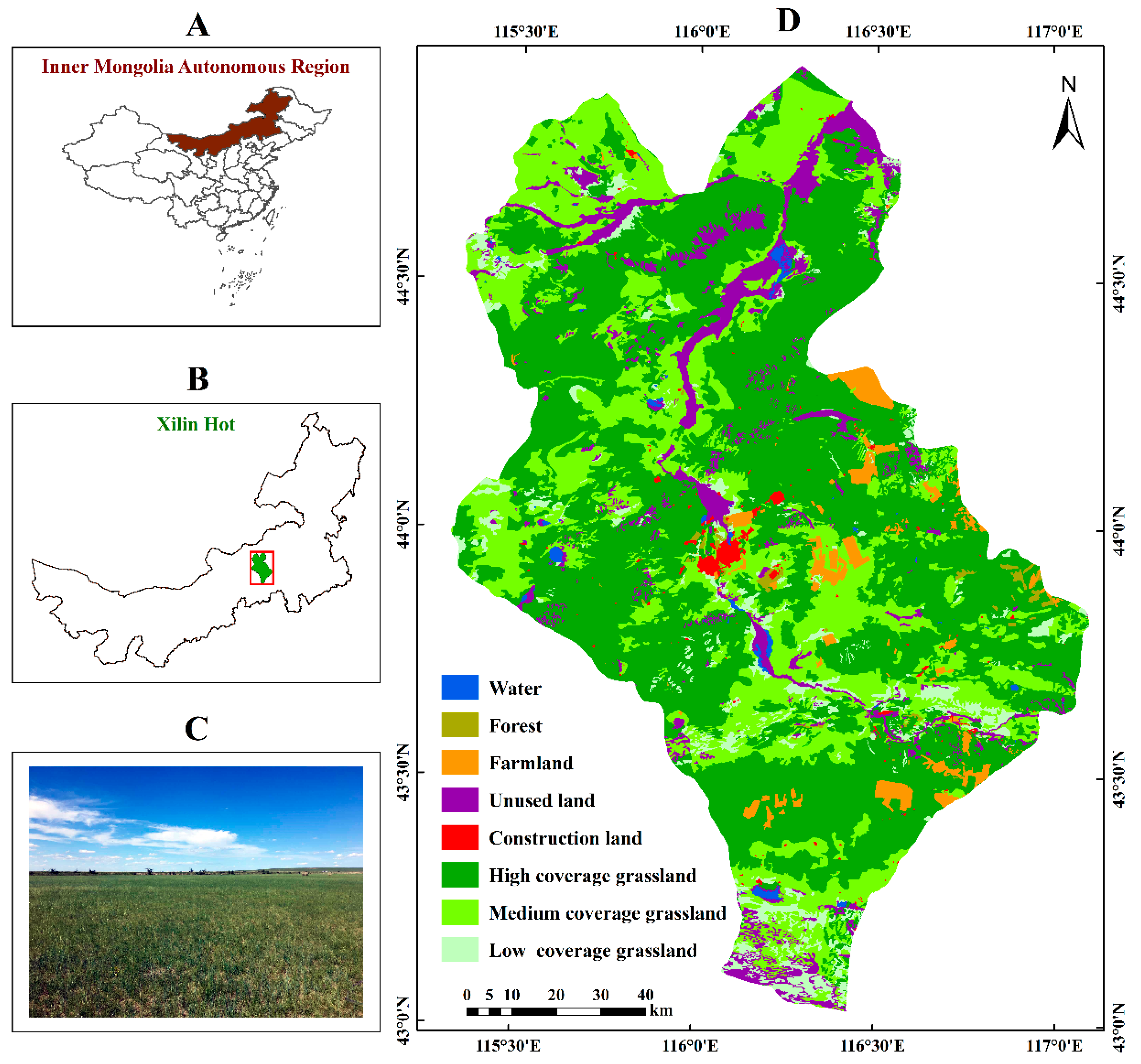
2.1. Study Area

Xilinhot is a prairie landscape city in central Inner Mongolia (43°02′–44°52′ N and 115°18′–117°06′ E) and covers a total area of 14,785 km2 (Figure 1A,B). The terrain is hilly in the South with gently undulating plains in the North and the average altitude is 988.5 m. The study area is located in the arid and semi-arid climate zone, which is characterized by cold temperatures, frequent drought, and strong wind [41]. The annual average temperature is stable at 0–3 °C, and July is the hottest month (21 °C). The average annual precipitation (PPT) is 295 mm, and much of the PPT occurs in July and August due to the large seasonal variability of this region. As the core area of XilinGol Grassland National Nature Reserve in China, the zonal soil is chestnut soil and the zonal vegetation is the temperate steppe dominated by xerophilous and bunch grass. The main constructive species and dominant species of steppe vegetation are Stipa grandis, S. kiriensis, Leymus chinensis, etc. Taking land use patterns of Xilinhot in 2010 as an example (Figure 1D), grasslands accounted for 88.63% of the total study area, followed by unused land (including sand land, bare land and saline land) (7.34%), farmland (2.43%), construction land (0.67%), open water (0.5%), and forests (including shrubs) (0.43%).

2.2. Quantification of ES and Data Sources

Specific features of the study region shaped our selection of the ES and ES assessment indicators used in this study. There is a fact that the study area is not only an important livestock production base in China, but also the priority implementation area of some ecological projects, including the Grain for Green Program (GFGP). During China’s 12th Five-Year Plan, a social and economic development initiative lasting from 2011–2015, ecological restoration policies implemented in Inner Mongolia prairie area focused on returning farmland to grasslands, implementing rotational grazing and zoning, and prohibiting over-grazing. The study area lies within the Northern part of the Beijing-Tianjin region, an area prone to soil erosion by water and wind, where the government launched a comprehensive watershed management project (Beijing-Tianjin Sandstorm Source Control Project) to prevent grassland degradation and desertification [42]. Therefore, our selection of ES was based on the following two considerations: (1) The indicators should be importance of the region’s social economy (e.g., animal husbandry is a pillar industry in the region); and (2) the indicators should represent the special status as a barrier of ecologic safety in Northern China.
In the end, we selected eight ES indicators, covering a range of provisioning services (grass production, livestock density, and water yield), regulating services (soil conservation, sand fixation, and carbon storage), maintenance services (habitat quality), and cultural services (landscape aesthetics) using the Millennium Ecosystem Assessment (MEA) classification systems (Table 1). In this paper, we mapped the physical quantity for each ES at 2010 to make sure we can analyze the ES supply under the same time node. In order to map each ES in the spatially explicit solution, we use an evaluation model or production function to quantify each ES based on high spatial resolution data. Table 1 provides quantitative methods and references for all services. The detailed description of the quantification of services is given in Supplementary Materials.
The main data used in this study were summarized in Table 2. Based on the ArcGIS (Version 10.3), using tools including reprojection, rasterization, and resampling, all data were unified by a projection coordinate system and a spatial resolution of (30 m in this study), thus we established the standardized spatial database of research area.

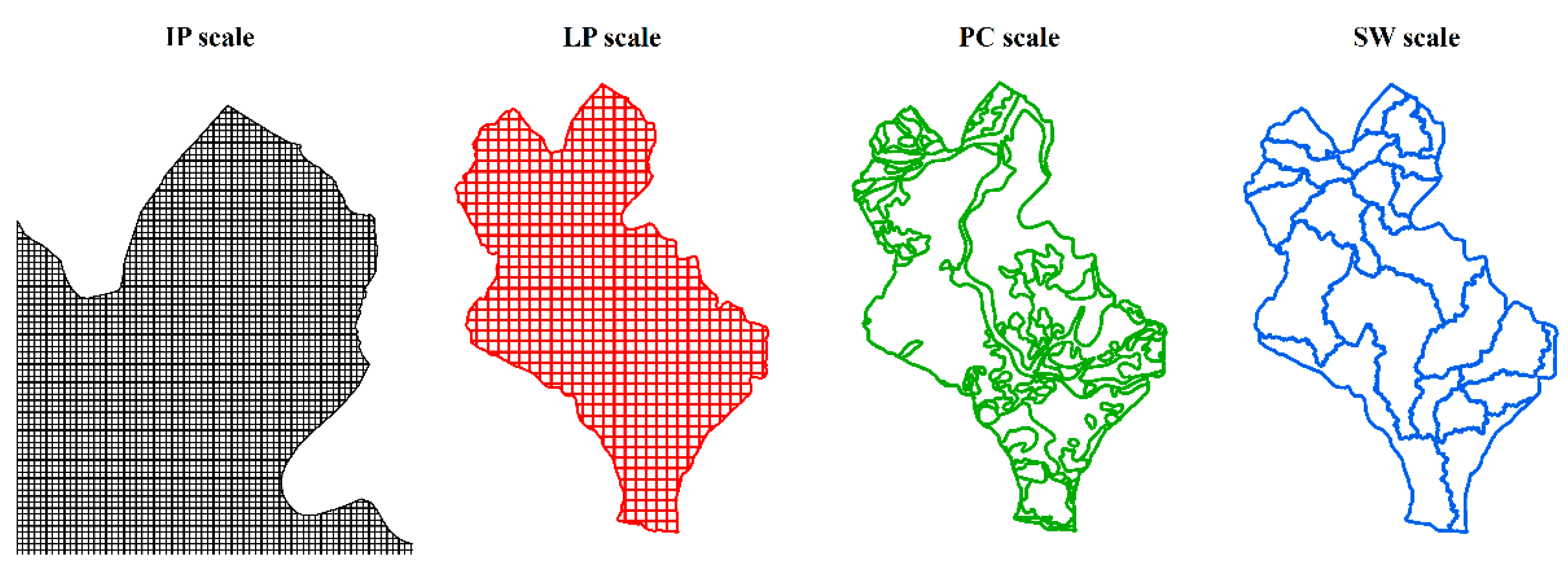
2.3. Setting Space Scales of Multiple Levels

We had the choice of multiple spatial scale here due to three considerations, including the extent limit of the study area, the spatial resolution of the model input data, and the relationship between the ES and the relevant scales. We finally chose four scales to represent different grain sizes and ecological hierarchies, and their spatial distribution was shown in Figure 2. The individual point (IP) scale (1 km grid) is the most commonly used scale in current research, representing the smallest observation and analysis scale in many ES mapping studies [34,35,39]. We chose a 1 km grid as the point scale because the original data of livestock density is based on a 1 km grid and the land use pattern of grassland is not as fragmented as in urban areas. The landscape patch (LP) scale (5 km grid) corresponds to the scale of plant microhabitats and this size is equivalent to the unit of pasture that each herdsman family can manage. The plant community (PC) scale is a completely natural, and is controlled by the biophysics properties of the dominant population. The sub-watershed (SW) scale represents a type of geomorphic scale and is currently the minimum scale used in ecological restoration projects for wind and water erosion in the study area [41,42,43]. We did not add a spatial level of administrative division scale, such as a village or township scale, because administrative boundaries may fluctuate throughout recent years.
Vector map layers at the IP scale (1 km grid) and LP scale (5 km grid) were both created using the Fishnet tool in ArcGIS. Vector range of the PC scale was represented by vegetation community regionalization data directly. The SW scale used the vector range of sub watershed, which was obtained by using the Soil and Water Assessment Tool (SWAT) based on DEM data. The conversion process of ES data from fine scale to coarse scale was based on the Zonal Statistics tool in ArcGIS, so we can extract the statistical values of all ES raster layers within the vector zones of four spatial scales. In addition, the average value method was used to extract raster values [44].

2.4. Data Analysis

After the mapping of the eight ES, we set the range of each ES raster data to a fixed scale (for example, 0–1 in this study) by the method of min–max normalization for the convenience of data management and analysis [20,21,45]. The spatial clustering of each ES was determined using both global and local Moran’s I with queen contiguity (i.e., common borders and corners) to visualize and compare spatial distribution patterns [39]. Correlation analysis was performed on each pair of services in R statistical software [46]. Due to the nonlinear and non-normal characteristics of geospatial data distribution, Spearman’s rank correlation analyses and corresponding significance tests were implemented using the “Hmisc” R package. Positive and negative correlations, respectively, represented the relationship of synergy and trade-off between pairwise ES. The absolute value of correlation coefficient changed from small to large, which represented the internal relationship between paired ES from weak to strong. We used the “psych” R package to conduct visualization treatments on the scatter distribution and correlation coefficient matrices for the data.
In order to identify ESB accurately, we have adopted two steps, including Principal Component Analysis (PCA) and Self-Organizing Map (SOM). As a precursor to cluster analysis, PCA is perfect for our dataset with multiple ES variables because an approximate linear relationship was commonly found between different ES variables in this study. Based on the principle of dimensionality reduction and ordination, this method can capture the variability in the dataset by transforming spatially correlated ES into uncorrelated several bundles of ES [47]. Subsequently, the main multivariate relationships among ES variables were quantified to assess whether multiple ES could co-exist in a certain ESB [48]. The load map of principal components provided guidance for more stable clustering solutions. We applied the SOM method to identify the ecosystem service bundles on account of its robustness to abnormal values and strong non-linearity mapping capacity [49]. Consequently, we used the “kohonen” R package to learn and train dataset to cluster locations of space cells objectively according to their similarity in multi-ES supply. In order to avoid the local optimal solution, we set the number of training to ten times the number of space cells, the initial learning rate and the final learning rate are 0.05 and 0.01, respectively. The algorithm of SOM was parametrized to build three to eight clusters at each scale, respectively, and we then used the Silhouette Width Index (SWI) to determine the optimal number of clusters [34]. The “starplot” R function was used to visualize the provision of ecosystem services by different clusters. The optimal clustering results will be mapped to vector data of different scales to visualize the spatial distribution pattern of the ecosystem service bundles.

3. Results

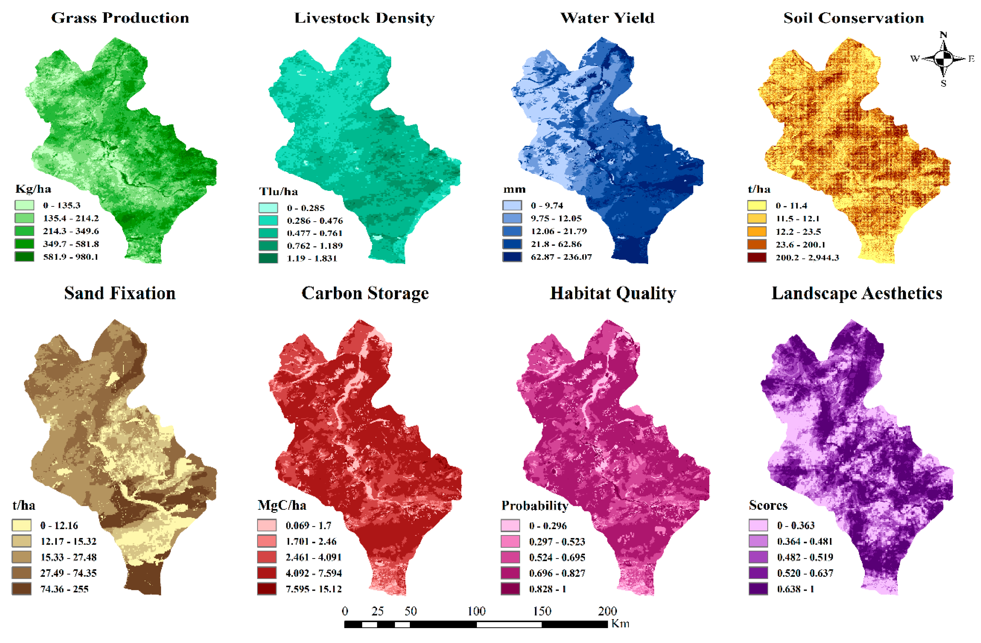
3.1. Spatial Distribution of Ecosystem Services Supply

While there are certain similarities in terms of the spatial characteristics of different ES (such as CS and HQ), each ES showed unique spatial characteristics in maps of ES supply distribution (Figure 3). For example, the spatial distribution of the GP supply increased from a low level in the West to a higher level in the East, while the spatial distribution of LD and WY gradually decreased from a high level in the Southeast to a lower level in the Northwest. In particular, the decrease in WY was the most obvious.

3.2. Individual Ecosystem Service Patterns

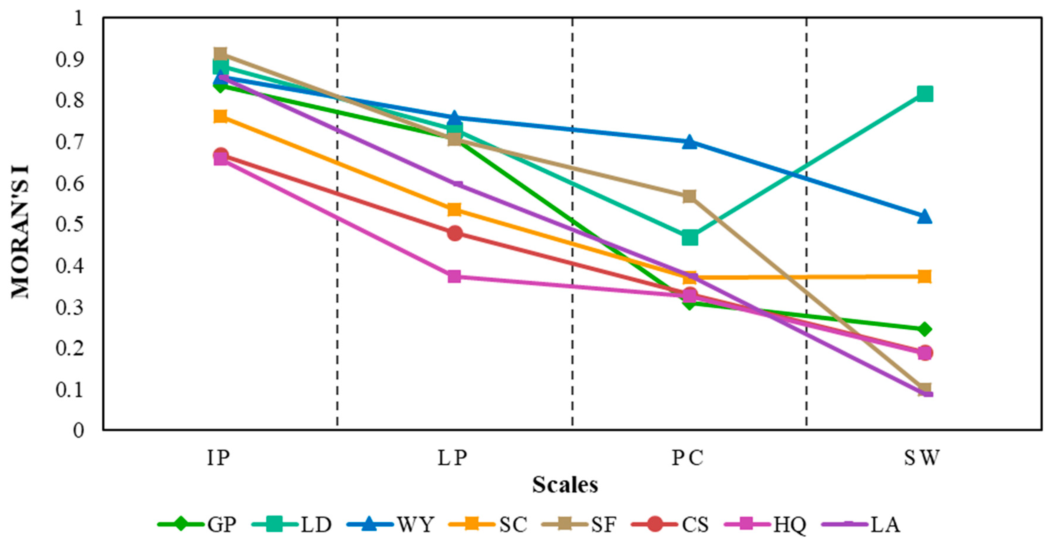
3.2.1. Global Moran’s I

Global Moran’s I results for all ES at each spatial scale were shown in Figure 4 and indicate that not all eight ES were spatially clustered across the four spatial scales (p < 0.01). Nearly all ES showed a pattern of decreasing clustering as the scale of observation increased. One exception was the LD service, which displayed an increase in clustering between the PC and SW scales. This is likely due to the clustering of water sources in only a few catchments or sub-watersheds and the high water requirements of large livestock, such as cattle, increased their density near water source sites in the research area [50]. These results support the hypothesis that certain ES may have similar spatial distributions at different spatial scales, and the cluster effect of ES supply may be caused by aggregate geographical endowment [28,51].

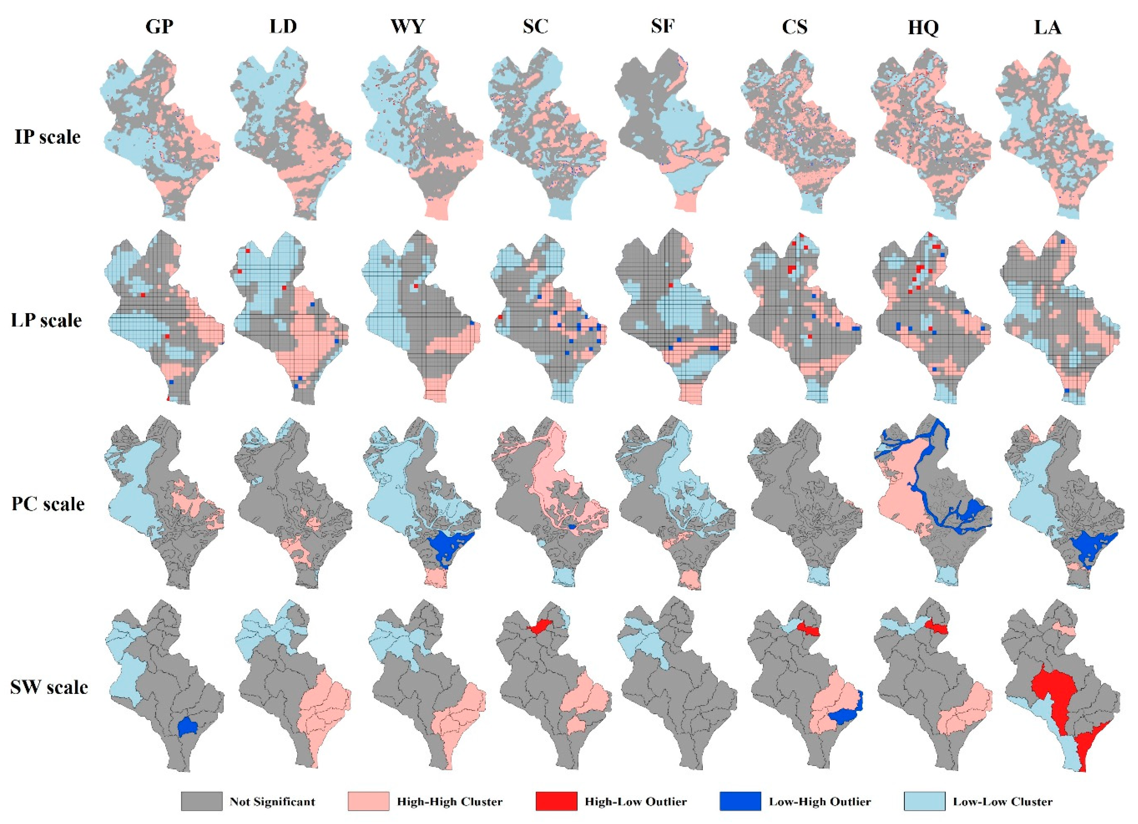
3.2.2. Anselin Local Moran’s I

Anselin Local Moran’s I was used to further explore statistically significant hot or cold spots and spatial outliers for all eight ES at the four different spatial scales (Figure 5). We found that, at the two finer scales (IP and LP scales), local spatial clustering patterns were dominated by High-High Cluster and Low-Low Cluster, while High-Low Outlier and Low-High Outlier associations were rare. However, there was a tendency that the High-Low Outlier and Low-High Outlier patterns increased sharply at coarser scales. This is because the smaller and isolated hot spots (High-High Cluster) or cold spots (Low-Low Cluster) are prone to be cut or filled at coarser scales [39]. Nevertheless, at the SW scale, the hot spots of LD and WY have a large overlap area, which further validated our interpretation of livestock clustering.

3.3. Pairwise Ecosystem Services Interactions

3.3.1. Significance of Trade-Offs and Synergies

We analyzed a total of 28 potential pairwise ES and their interactions among the eight ES (Figure 6). Apparently, as the scale became coarser, accompanied by the decreased number of pairwise ES that could still maintain significant correlation (p < 0.05). At the IP scale, 27 pairs were significantly correlated with each other, and this number only dropped to 26 at the LP scale. However, as the scale became the PC scale, the number rapidly dropped to only 18, and further decreased to 12 at the SW scale. Only one pair, CS-HQ, kept very significantly correlative with each other at all four scales (p < 0.001). This was because the results of significance tests were easily impacted by the sample size, which decreased exponentially from fine to coarse scales as the numbers of spatial units at the four scales were 16,172, 712, 86, and 22 respectively. At the same time, we found that the number of ES pairs with significant negative correlation was decreasing in the process of scaling up (p < 0.05). There was only a significant trade-off between the SC and LA services at the SW scale.

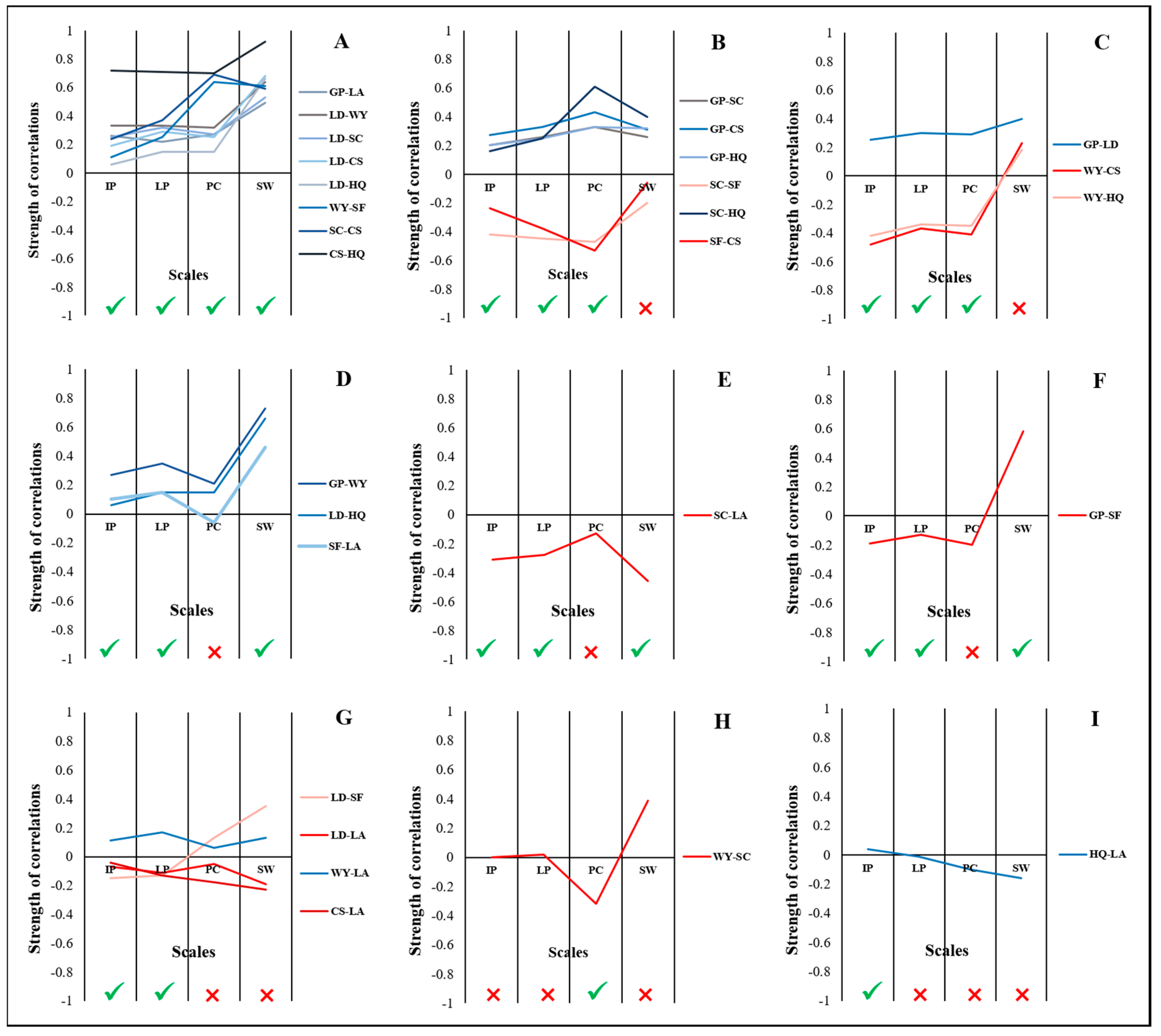
3.3.2. Strength of Trade-Offs and Synergies

We summarized nine styles of change trends in this study by which the relationship between pairwise ES has changed in the process of upscaling (Figure 7A–I). The vast majority of paired ES, which shows a positive correlation, the strength of correlation increased in the intervals with significance. However, for pairwise ES interactions showing negative correlations, the strength change of correlation has relative uncertainty in the intervals with significance including unidirectional decreases or increases, or an initial decrease followed by an increase. It is worth noting that WY-SC did not pass the significance test at the IP, LP, or SW scales, and it showed no correlation (|r| ≤ 0.1) at both IP and LP scales. Nevertheless, this pair showed a significantly moderate trade-off at the PC scale (−0.5 < r ≤ −0.3). Such results also verified that the relationship between pairwise ES may be easily missed at one single scale. However, although HQ-LA showed similar relationship changes, we generally thought that there was no correlation between these two services, because correlation coefficient at the IP scale was much smaller than 0.1.

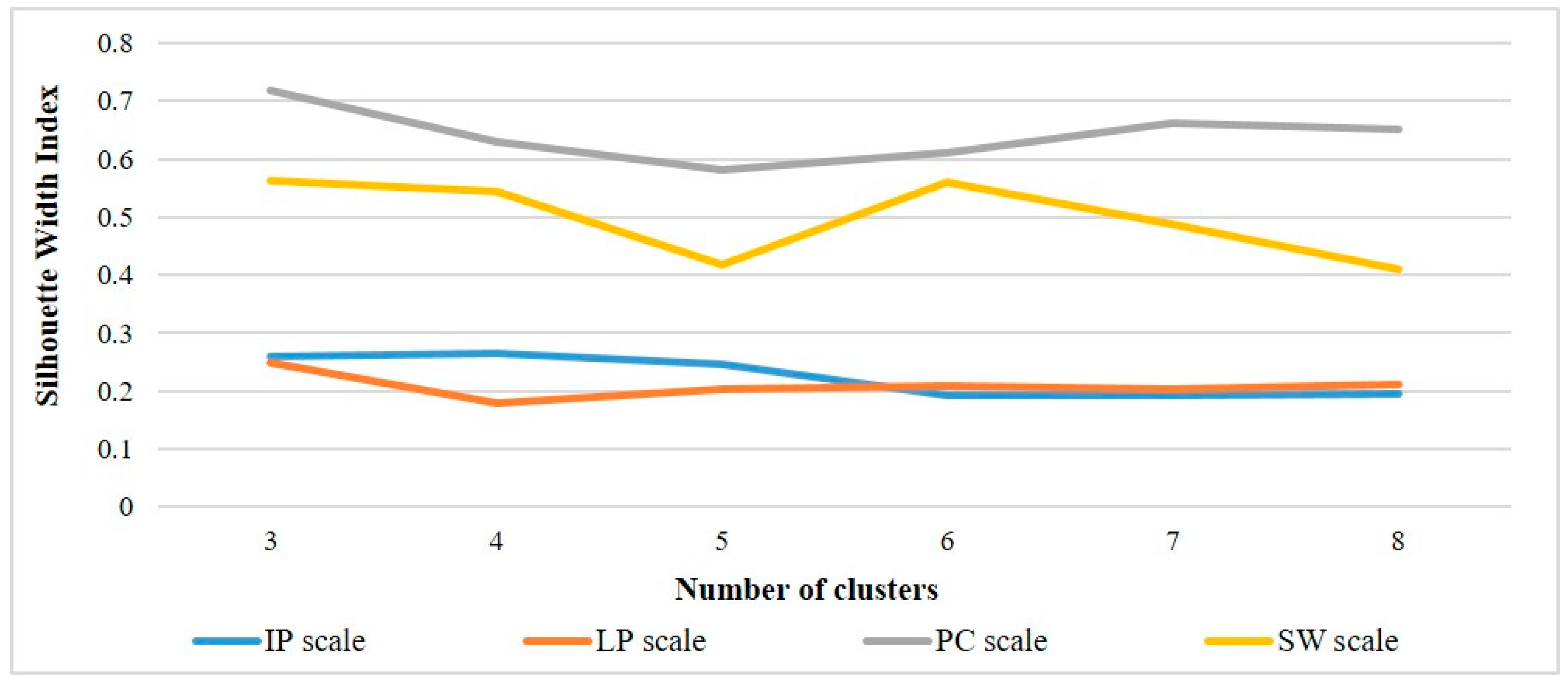
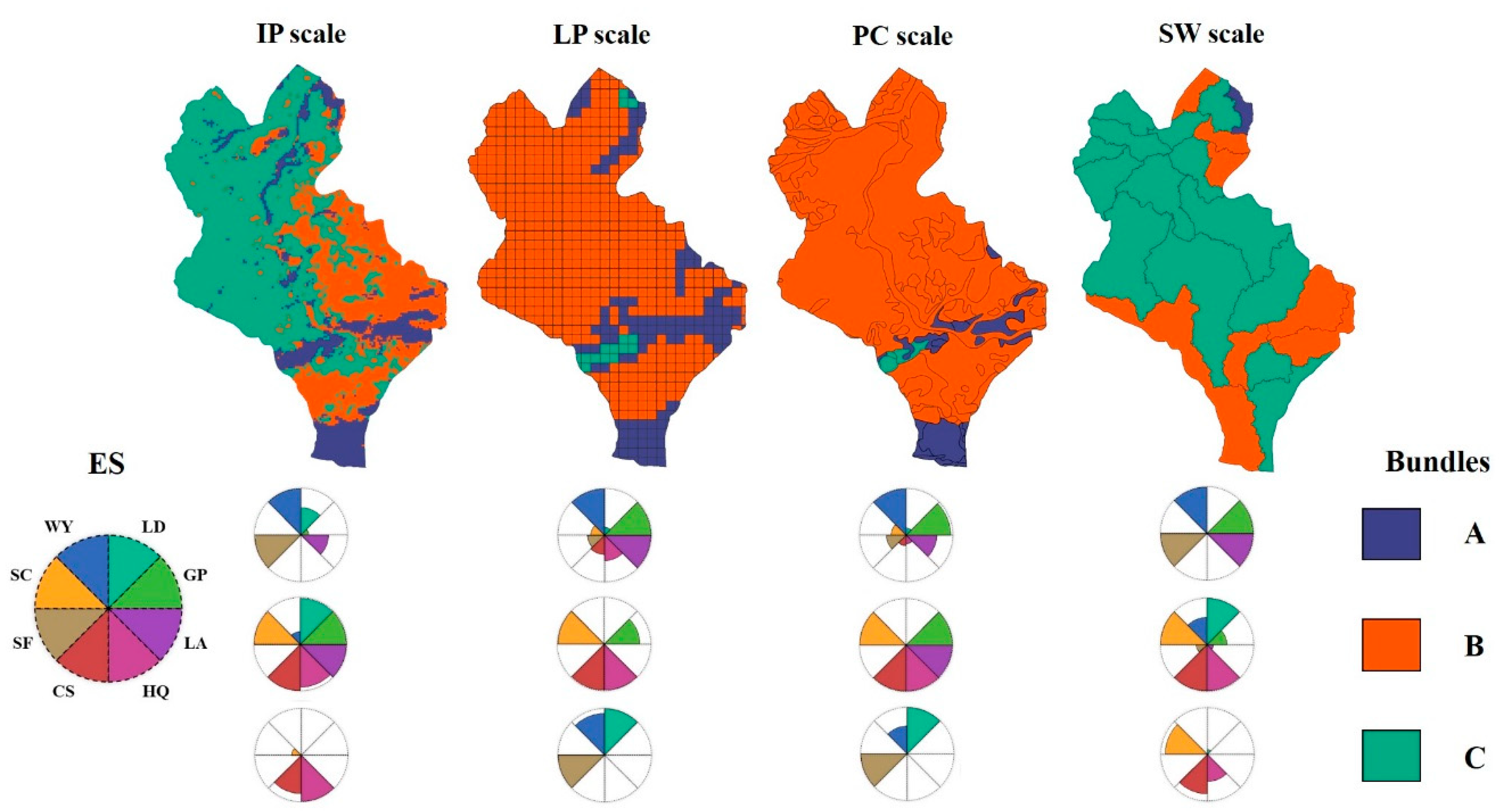
3.4. Ecosystem Service Bundles

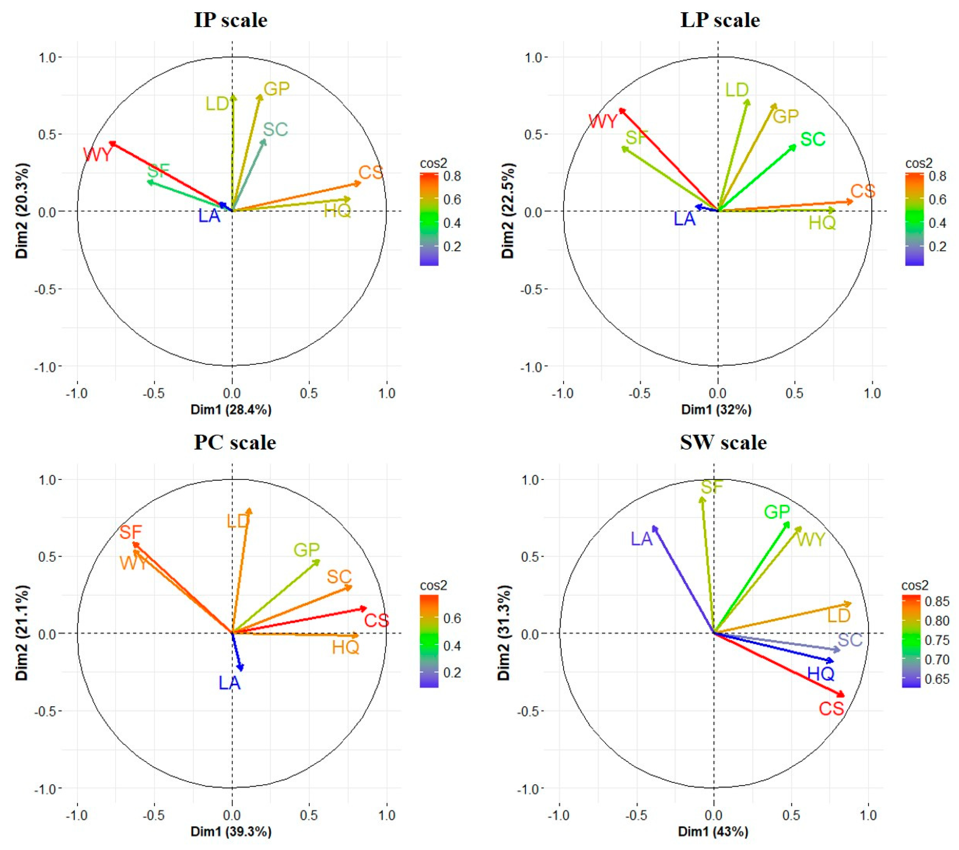
3.4.1. Multivariate Relationships

As shown in Figure 8, most ES could be fully explained by the first two main component axes Dim1 and Dim2, while the interpretation axes of some specific ES (e.g., LA) could be found in higher-order principal components. However, in general, higher-order principal components were negligible because they only accounted for a small part of the variance and mainly contained random changes. There was a clear trend that, as spatial scale became coarser, the percentage of the total variance that could be explained by the first two principal components increased. At the IP scale, the first two principal components could explain 48.7% of the total variance. However, at the SW scale, the first two principal components could explain 74.3% of the total variance. However, the ES with the highest representativeness underwent major changes as the spatial scale changes. At the IP and LP scales, WY has the highest representativeness. Meanwhile the representativeness of SF and SC was weaker at these two scales because they were highly affected by vegetation and terrain conditions, which showed weaker spatial heterogeneity in the study area at the finer spatial scales (i.e., 1 km2 or 5 km2 cells). However, at the relatively coarse PC scale, SF and CS showed the highest representativeness.

3.4.2. Spatially Explicit Bundles

Based on map visualization, our SOM results revealed that the process of ESB formation by multiple ES was clearly dependent on spatial scale. We found that the clustering results at the PC scale always maintained the highest value of SWI among all scales, which provided the best separation effect between the clusters (Figure 9). In terms of the optimal clustering solutions at each scale, except the number of four clusters was associated with the highest SWI value of 0.264 at the IP scale. In order to compare the combination and distribution of ESB at different scales more intuitively, we uniformly set the number of clusters to three. We found that, with the changing scale, the component and spatial distribution location of each class of ESB were markedly different (Figure 10). Taking the Class A bundle as an example, SF supply was relatively strong in class A at the IP and SW scales, while it was quite weak at the LP and PC scales. On the SW scale, Class A bundle could not be identified in the South of the study area, but Class A bundle was identified in the same location at the first three scales. Moreover, we can see that with the scale change, the area proportion of different classes of ESB has also changed.

4. Discussion

4.1. The Scale Effect of Ecosystem Services Supply

In this study, the random distribution of several ES, including HQ and LA, could be seen at coarse spatial scales. Similar distributions were observed for the education service in the Yangtze River Delta region of China [20], and the tourism service in the Quebec region of Canada [35]. We found that randomly distributed ES can be provided directly or influenced indirectly by semi-natural and artificial systems, which are often under intense human modification in large scale research units (such as the expansion of construction land and grazing intensity of pasture in this study). While previous findings shows that the spatial pattern of ES supply can be optimized through human configuration, we must be alert to that discrete distribution of ES hotspots may lead to spatial mismatches between supply and demand in local ecosystem management [52]. A better understanding of the spatial clustering characteristics of ES could provide managers useful information to decide where to improve the supply of which ES at a particular scale.
When performing data integration of ES from a fine scale to a coarse scale, it may hinder local trade-offs between ES, especially when different ES exhibit spatial competition. Xu found that the ES of food supply and tourism generated trade-offs at fine spatial scales (≤7 km), but such trade-offs became synergies at a coarser spatial scale (>7 km) because the supply sources of tourism have increased at a coarser scale (water area is also considered a kind of tourism resource) [39]. In our research, the same phenomenon was found between GP and SF, while this pair changed from trade-off (at the IP and LP scales) to synergy (at the SW scale). This is because large-scale units in the study can make the impact of meteorological factors such as wind speed and precipitation on these two services more significant, and the ability of high coverage vegetation weakening wind erosion can be brought into full play, while small-scale units may only form a local trade-off between these two services through topographic conditions. This explanation is based on the niche complementary effect in ecology in which a multi-species mixture, compared with a monoculture, can make full use one or more resources in the system to achieve higher productivity and benefits [20,38]. Therefore, the units often include a greater number and type of ES at coarse scales. It is worth noting that there are most pairs of moderate and high trade-offs with significance at the PC scale (r ≤ −0.3), which might be caused by the spatial competition among different plant populations in grasslands. The relationships between ES, highly affected by the variability of vegetation characteristics, may be more easily observable in correlation analysis.
While we clustered three class of ESB, their degree of cluster separation identified at the four spatial scales was quite different. The SOM results obtained at the PC scale provided the highest SWI value (0.719), which was much larger than the corresponding values obtained at the other three scales. The PC scale also provided the highest degree of separation among clusters, indicating that the PC scale may provide a more reliable result for ESB identification in the study area. Since water is the most important factor in local development in arid regions, the PCA results obtained at the PC scale showed that the variance explained by WY was the highest among all eight ES variables. Therefore, in SOM, WY-dominated clusters (Class A Bundles) were most likely to be separated. ESB revealed that, in the typical steppe areas with arid and semi-arid climate, population distribution and grassland evolution, compared to LULC, played a more significant role in driving the spatial combination of multiple ES. Since the biophysical characteristics of different types of vegetation are significantly different, such as water consumption, evaporation, soil consolidation, and palatability to livestock [53,54,55]. The coupling of multiple factors leads to the selection of scale is different from that of other regions with higher urbanization level. If only using the regular grid scale, we cannot accurately reveal associations among ES supply. Thus, a multi-scale analysis is necessary for us to obtain a more robust result in pairwise ES interactions and ES bundles.

4.2. Uncertainties in Scaling-Up Process

Uncertainties in ES modelling and underlying measurements have been widely discussed in many studies [56]. However, scaling-up process or approaches can also bring uncertainty [57]. Firstly, the problem of how to cluster ES from a fine scale to a coarse scale deserves wide attention. In this paper, we provided a solution based on GIS. The premise of this approach is to use polygon vector and zonal statistics to extract ES data at each scale, which is also a common sampling method in multiscale analysis. While some studies used random points to extract ES data at multiple scales, it remains questionable as to whether the results of random points at a coarser scale can reflect the overall condition of the ‘units’ due to the nugget effect. The nugget effect tends to originate from errors due to data with different spatial resolutions when we are sampling or resampling at different distances [58]. However, heterogeneity and inherent variability of different ES dominated the different nugget effects, which remains to be understood and solved.
Secondly, the choice of spatial scales depends on the process of ES selection, while the resolution of ES quantification depends on the quantized model and input data, which limits the choice of the minimum scale. However, if multiple ES closely related to human activities are assessed in a large regional area (such as tourism service), it is often necessary to select the scales corresponding to multiple administrative regions, such as towns and cities [59]. For example, the IP scale used in this study was a one km grid based on the following two reasons. First, it was constrained by the resolution of LD data. Second, a smaller scale would exponentially increase the amount of data (the 30 m scale would generate more than 200,000 grid data), which would create a heavy burden of computing. Therefore, the selection of one km as the individual point scale here was more of a compromise. However, the assessment resolution of some other services was less than one km. For example, the resolution of GP is 250 m and the resolution of CS is 30 m. Therefore, the setting of minimum scale to one km could easily lead to the loss of internal fluctuation details in some units with small resolution elements (LUCC and NDVI). This is the most easily overlooked source of uncertainty. However, with the increased resolutions in the data, such as land use, meteorology, and soil data, as well as further calibration of model parameters, the uncertainty will gradually decrease in future research.

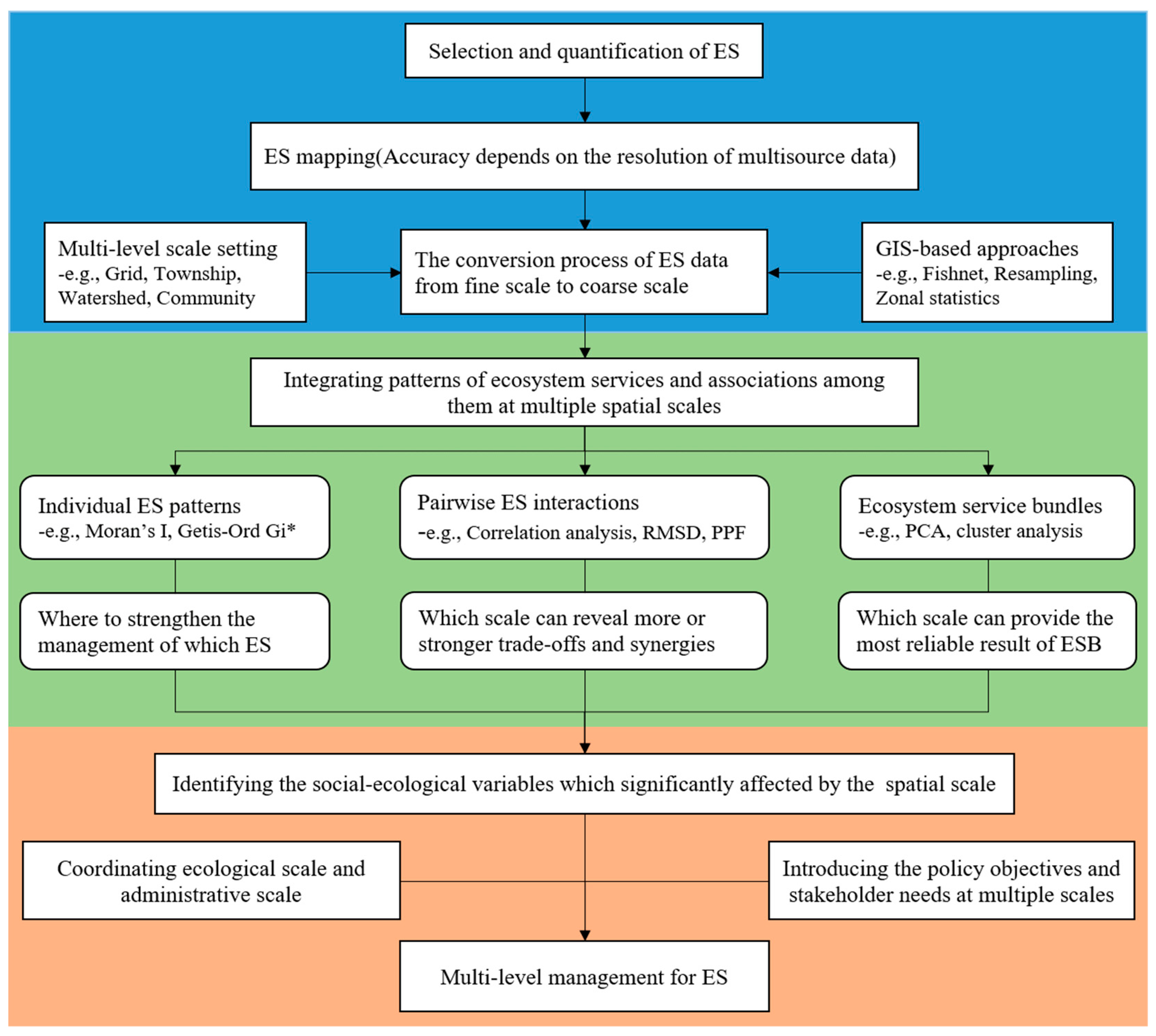
4.3. A Framework for Integrating Patterns of Ecosystem Services and Associations among Them at Multiple Spatial Scales

The integration of the ES concept in decision-making has been increasingly promoted in the scientific literature, as well as in policy guidelines at different strategic levels [60]. Most of the previous studies have focused on how to integrate ES into social values [61], or how to include ES and human welfare into the framework of management practice [18]. However, few researchers have noticed the scale effect during evaluating the ES supply process. Based on our results, we have established a framework to integrate spatial patterns of ecosystem services and associations among them at multiple scales (Figure 11).
In this framework, we need to solve a core issue about how to detect the scale effect. In this study, we have coordinated the analysis routes in three areas. In terms of individual ES pattern, the results of cold and hot spot identification are relatively intuitive when the popular methods of Moran’s I and Gi* statistics are used [62]. We used a relatively simple correlation analysis to quantify pairwise ES interaction and its strength. Of course, the recently proposed statistical models, such as Root Mean Square Error (RMSE) [63,64] and Production Possibilities Frontier (PPF) [65], can also be used to describe such relationship more accurately, which depends on the actual situation of ES distribution in the study area. Many researchers have used cluster analyses to identify ESB, however, the algorithm of cluster analysis and the number of clusters needs to be subjectively determined. Therefore, the exploratory nature of cluster analysis makes it unsuitable for understanding the causality in the associations among multiple ES. It is necessary to perform PCA before clustering, so as to visualize major multivariate relationships.
Finally, social and ecological variables, which can affect ES supply at different scales, should be identified. Currently, the understanding regarding the differences among social and ecological variables at different scales, as well as the driving mechanisms of ES trade-offs, is scarce and should be urgently solved to characterize and explain the cross-scale correlation between these factors [5]. Furthermore, we can introduce the policy objectives and stakeholder needs at multiple scales, so as to co-ordinate ecological scales and administrative scales in the multi-level management of ES [66]. We will carry out relevant studies in the next step.

5. Conclusions

It is necessary to understand the effects of spatial scale on the measurement, analysis, and management of ES. We set up our study area in a city in Inner Mongolian dominated by natural grassland landscape. Based on the quantification and mapping of eight representative ecosystem services, we set up four levels of spatial scale to detect scale effect on ES supply. The results showed that scale effect of ES supply can be revealed in three aspects, including individual ES patterns, pairwise ES interactions, and ecosystem service bundles (ESB). This study proved that single-scale analysis can only capture the limited information of the ES supply pattern at a certain scale. Because the degree of heterogeneity of the spatial unit cannot be clarified, it may lead to distortion or omission of the relationship among certain ES. Our research has provided a framework to integrate patterns of ecosystem services and associations among them at multiple spatial scales. This framework is expected to be used in other regions or other types of ecosystems around the world, so that the trend of changes in this scale effect can be further tested and the results can provide an important reference for policy-makers to coordinate different scales. Our future work will focus on clarifying the driving mechanisms of tradeoffs and synergies at different scales.

Supplementary Materials

The following are available online at https://www.mdpi.com/2071-1050/10/10/3654/s1.

Author Contributions

Conceptualization, H.D. and X.L.; Formal analysis, H.D.; Resources, S.L.; Software, D.D.; Writing—original draft, H.D.; Writing—review & editing, X.L. and S.L.

Funding

This work was financially supported by the National Key Research and Development Program of China (No. 2016YFC0500502), the Natural Science Foundation of China (No. 31570451), and the Program for Changjiang Scholars and Innovative Research Team in University (No. IRT_15R06).

Acknowledgments

We thank two anonymous reviewers for their valuable comments on an earlier version of the paper. This work was financially supported by the National Key Research and Development Program of China (No. 2016YFC0500502), the Natural Science Foundation of China (No. 31570451), and the Program for Changjiang Scholars and Innovative Research Team in University (No. IRT_15R06).

Conflicts of Interest

The authors declare no conflict of interest.

References

  1. Millennium Ecosystem Assessment (MEA). Ecosystems and Human Well-being: Synthesis; Island Press: Washington, DC, USA, 2005; ISBN 978-159-726-711-3. [Google Scholar]
  2. Tallis, H.; Kareiva, P.; Marvier, M.; Chang, A. An ecosystem services framework to support both practical conservation and economic development. Proc. Natl. Acad. Sci. USA 2008. [Google Scholar] [CrossRef] [PubMed]
  3. Malinga, R.; Gordon, L.J.; Jewitt, G.; Lindborg, R. Mapping ecosystem services across scales and continents—A review. Ecosyst. Serv. 2015, 13, 57–63. [Google Scholar] [CrossRef]
  4. Costanza, R.; De Groot, R.; Braat, L.; Kubiszewski, I.; Fioramonti, L.; Sutton, P.; Farber, S.; Grasso, M. Twenty years of ecosystem services: How far have we come and how far do we still need to go? Ecosyst. Serv. 2017, 28, 1–16. [Google Scholar] [CrossRef]
  5. Spake, R.; Lasseur, R.; Crouzat, E.; Bullock, J.M.; Lavorel, S.; Parks, K.E.; Schaafsma, M.; Bennett, E.M.; Maes, J.; Mulligan, M.; et al. Unpacking ecosystem service bundles: Towards predictive mapping of synergies and trade-offs between ecosystem services. Glob. Environ. Chang. 2017, 47, 37–50. [Google Scholar] [CrossRef]
  6. Hauck, J.; Albert, C.; Fürst, C.; Geneletti, D.; La Rosa, D.; Lorz, C.; Spyra, M. Developing and applying ecosystem service indicators in decision-support at various scales. Ecol. Indic. 2016, 61, 1–5. [Google Scholar] [CrossRef] [Green Version]
  7. Jarvis, P.G. Scaling processes and problems. Plant Cell Environ. 1995, 18, 1079–1089. [Google Scholar] [CrossRef]
  8. Rivera, J.M.; Muñoz, M.J.; Moneva, J.M. Revisiting the Relationship Between Corporate Stakeholder Commitment and Social and Financial Performance. Sustain. Dev. 2017, 25, 482–494. [Google Scholar] [CrossRef] [Green Version]
  9. Syrbe, R.U.; Walz, U. Spatial indicators for the assessment of ecosystem services: Providing, benefiting and connecting areas and landscape metrics. Ecol. Indic. 2012, 21, 80–88. [Google Scholar] [CrossRef]
  10. Burkhard, B.; Kroll, F.; Nedkov, S.; Müller, F. Mapping ecosystem service supply, demand and budgets. Ecol. Indic. 2012, 21, 17–29. [Google Scholar] [CrossRef]
  11. García-Nieto, A.P.; García-Llorente, M.; Iniesta-Arandia, I.; Martín-López, B. Mapping forest ecosystem services: From providing units to beneficiaries. Ecosyst. Serv. 2013, 4, 126–138. [Google Scholar] [CrossRef]
  12. Boithias, L.; Acuña, V.; Vergoñós, L.; Ziv, G.; Marcé, R.; Sabater, S. Assessment of the water supply: Demand ratios in a Mediterranean basin under different global change scenarios and mitigation alternatives. Sci. Total Environ. 2014, 470–471, 567–577. [Google Scholar] [CrossRef] [PubMed]
  13. Wolff, S.; Schulp, C.J.E.; Verburg, P.H. Mapping ecosystem services demand: A review of current research and future perspectives. Ecol. Indic. 2015, 55, 159–171. [Google Scholar] [CrossRef]
  14. Luck, G.W.; Daily, G.C.; Ehrlich, P.R. Population diversity and ecosystem services. Trends Ecol. Evol. 2003, 18, 331–336. [Google Scholar] [CrossRef] [Green Version]
  15. Zheng, H.; Robinson, B.E.; Liang, Y.-C.; Polasky, S.; Ma, D.-C.; Wang, F.-C.; Ruckelshaus, M.; Ouyang, Z.-Y.; Daily, G.C. Benefits, costs, and livelihood implications of a regional payment for ecosystem service program. Proc. Natl. Acad. Sci. USA 2013, 110, 16681–16686. [Google Scholar] [CrossRef] [PubMed] [Green Version]
  16. Rozas-Vásquez, D.; Fürst, C.; Geneletti, D.; Almendra, O. Integration of ecosystem services in strategic environmental assessment across spatial planning scales. Land Use Policy 2018, 71, 303–310. [Google Scholar] [CrossRef]
  17. Lin, Y.P.; Lin, W.C.; Wang, Y.C.; Lien, W.Y.; Huang, T.; Hsu, C.C.; Schmeller, D.S.; Crossman, N.D. Systematically designating conservation areas for protecting habitat quality and multiple ecosystem services. Environ. Model. Softw. 2017, 90, 126–146. [Google Scholar] [CrossRef]
  18. Wang, B.; Tang, H.; Xu, Y. Integrating ecosystem services and human well-being into management practices: Insights from a mountain-basin area, China. Ecosyst. Serv. 2017, 27, 58–69. [Google Scholar] [CrossRef]
  19. Fu, B.; Liu, Y.; Lü, Y.; He, C.; Zeng, Y.; Wu, B. Assessing the soil erosion control service of ecosystems change in the Loess Plateau of China. Ecol. Complex. 2011, 8, 284–293. [Google Scholar] [CrossRef]
  20. Yang, G.; Ge, Y.; Xue, H.; Yang, W.; Shi, Y.; Peng, C.; Du, Y.; Fan, X.; Ren, Y.; Chang, J. Using ecosystem service bundles to detect trade-offs and synergies across urban-rural complexes. Landsc. Urban Plan. 2015, 136, 110–121. [Google Scholar] [CrossRef]
  21. Kong, L.; Zheng, H.; Xiao, Y.; Ouyang, Z.; Li, C.; Zhang, J.; Huang, B. Mapping ecosystem service bundles to detect distinct types of multifunctionality within the diverse landscape of the Yangtze River Basin, China. Sustainability 2018, 10, 857. [Google Scholar] [CrossRef]
  22. Rabe, S.E.; Koellner, T.; Marzelli, S.; Schumacher, P.; Grêt-Regamey, A. National ecosystem services mapping at multiple scales—The German exemplar. Ecol. Indic. 2016, 70, 357–372. [Google Scholar] [CrossRef]
  23. Redhead, J.W.; May, L.; Oliver, T.H.; Hamel, P.; Sharp, R.; Bullock, J.M. National scale evaluation of the InVEST nutrient retention model in the United Kingdom. Sci. Total Environ. 2018, 610, 666–677. [Google Scholar] [CrossRef] [PubMed]
  24. Petz, K.; Alkemade, R.; Bakkenes, M.; Schulp, C.J.E.; van der Velde, M.; Leemans, R. Mapping and modelling trade-offs and synergies between grazing intensity and ecosystem services in rangelands using global-scale datasets and models. Glob. Environ. Chang. 2014, 29, 223–234. [Google Scholar] [CrossRef]
  25. Bennett, E.M.; Peterson, G.D.; Gordon, L.J. Understanding relationships among multiple ecosystem services. Ecol. Lett. 2009, 12, 1394–1404. [Google Scholar] [CrossRef] [PubMed] [Green Version]
  26. Howe, C.; Suich, H.; Vira, B.; Mace, G.M. Creating win-wins from trade-offs? Ecosystem services for human well-being: A meta-analysis of ecosystem service trade-offs and synergies in the real world. Glob. Environ. Chang. 2014, 28, 263–275. [Google Scholar] [CrossRef]
  27. Rodríguez, J.P.; Beard, T.D.; Bennett, E.M.; Cumming, G.S.; Cork, S.J.; Agard, J.; Dobson, A.P.; Peterson, G.D. Trade-offs across space, time, and ecosystem services. Ecol. Soc. 2006, 11. [Google Scholar] [CrossRef]
  28. Raudsepp-Hearne, C.; Peterson, G.D.; Bennett, E.M. Ecosystem service bundles for analyzing tradeoffs in diverse landscapes. Proc. Natl. Acad. Sci. USA 2010, 107, 5242–5247. [Google Scholar] [CrossRef] [PubMed] [Green Version]
  29. Haase, D.; Schwarz, N.; Strohbach, M.; Kroll, F.; Seppelt, R. Synergies, trade-offs, and losses of ecosystem services in urban regions: An integrated multiscale framework applied to the Leipzig-Halle region, Germany. Ecol. Soc. 2012, 17. [Google Scholar] [CrossRef]
  30. Turner, K.G.; Odgaard, M.V.; Bøcher, P.K.; Dalgaard, T.; Svenning, J.C. Bundling ecosystem services in Denmark: Trade-offs and synergies in a cultural landscape. Landsc. Urban Plan. 2014, 125, 89–104. [Google Scholar] [CrossRef]
  31. Sun, X.; Li, F.; Sun, X.; Li, F. Spatiotemporal assessment and trade-offs of multiple ecosystem services based on land use changes in Zengcheng, China. Sci. Total Environ. 2017, 609, 1569–1581. [Google Scholar] [CrossRef] [PubMed]
  32. Qin, K.; Li, J.; Yang, X. Trade-off and synergy among ecosystem services in the Guanzhong-Tianshui economic region of China. Int. J. Environ. Res. Public Health 2015, 12, 14094–14113. [Google Scholar] [CrossRef] [PubMed]
  33. Kang, H.; Seely, B.; Wang, G.; Innes, J.; Zheng, D.; Chen, P.; Wang, T.; Li, Q. Evaluating management tradeoffs between economic fiber production and other ecosystem services in a Chinese-fir dominated forest plantation in Fujian Province. Sci. Total Environ. 2016, 557–558, 80–90. [Google Scholar] [CrossRef] [PubMed]
  34. Mouchet, M.A.; Paracchini, M.L.; Schulp, C.J.E.; Stürck, J.; Verkerk, P.J.; Verburg, P.H.; Lavorel, S. Bundles of ecosystem (dis)services and multifunctionality across European landscapes. Ecol. Indic. 2017, 73, 23–28. [Google Scholar] [CrossRef]
  35. Raudsepp-Hearne, C.; Peterson, G.D. Scale and ecosystem services: How do observation, management, and analysis shift with scale—lessons from Québec. Ecol. Soc. 2016, 21. [Google Scholar] [CrossRef]
  36. Holland, R.A.; Eigenbrod, F.; Armsworth, P.R.; Anderson, B.J.; Thomas, C.D.; Heinemeyer, A.; Gillings, S.; Roy, D.B.; Gaston, K.J. Spatial covariation between freshwater and terrestrial ecosystem services. Ecol. Appl. 2011, 21, 2034–2048. [Google Scholar] [CrossRef] [PubMed]
  37. Comín, F.A.; Miranda, B.; Sorando, R.; Felipe-Lucia, M.R.; Jiménez, J.J.; Navarro, E. Prioritizing sites for ecological restoration based on ecosystem services. J. Appl. Ecol. 2018, 55, 1155–1163. [Google Scholar] [CrossRef]
  38. Liu, Y.; Bi, J.; Lv, J.; Ma, Z.; Wang, C. Spatial multi-scale relationships of ecosystem services: A case study using a geostatistical methodology. Sci. Rep. 2017, 7. [Google Scholar] [CrossRef] [PubMed] [Green Version]
  39. Xu, S.; Liu, Y.; Wang, X.; Zhang, G. Scale effect on spatial patterns of ecosystem services and associations among them in semi-arid area: A case study in Ningxia Hui Autonomous Region, China. Sci. Total Environ. 2017, 598, 297–306. [Google Scholar] [CrossRef] [PubMed]
  40. Goldstein, J.H.; Caldarone, G.; Duarte, T.K.; Ennaanay, D.; Hannahs, N.; Mendoza, G.; Polasky, S.; Wolny, S.; Daily, G.C. Integrating ecosystem-service tradeoffs into land-use decisions. Proc. Natl. Acad. Sci. USA 2012, 109, 7565–7570. [Google Scholar] [CrossRef] [PubMed] [Green Version]
  41. Hao, R.; Yu, D.; Liu, Y.; Liu, Y.; Qiao, J.; Wang, X.; Du, J. Impacts of changes in climate and landscape pattern on ecosystem services. Sci. Total Environ. 2017, 579, 718–728. [Google Scholar] [CrossRef] [PubMed]
  42. Du, H.; Dou, S.; Deng, X.; Xue, X.; Wang, T. Assessment of wind and water erosion risk in the watershed of the Ningxia-Inner Mongolia Reach of the Yellow River, China. Ecol. Indic. 2016, 67, 117–131. [Google Scholar] [CrossRef]
  43. Shi, Z.H.; Ai, L.; Fang, N.F.; Zhu, H.D. Modeling the impacts of integrated small watershed management on soil erosion and sediment delivery: A case study in the Three Gorges Area, China. J. Hydrol. 2012, 438–439, 156–167. [Google Scholar] [CrossRef]
  44. About ArcGIS | Mapping & Analytics Platform. Available online: https://www.esri.com/en-us/arcgis/about-arcgis/overview (accessed on 13 September 2018).
  45. Yang, W.; Dietz, T.; Liu, W.; Luo, J.; Liu, J. Going Beyond the Millennium Ecosystem Assessment: An Index System of Human Dependence on Ecosystem Services. PLoS ONE 2013, 8. [Google Scholar] [CrossRef] [PubMed]
  46. R: The R Project for Statistical Computing. Available online: https://www.r-project.org/ (accessed on 13 September 2018).
  47. Abson, D.J.; Dougill, A.J.; Stringer, L.C. Using Principal Component Analysis for information-rich socio-ecological vulnerability mapping in Southern Africa. Appl. Geogr. 2012, 35, 515–524. [Google Scholar] [CrossRef]
  48. Marsboom, C.; Vrebos, D.; Staes, J.; Meire, P. Using dimension reduction PCA to identify ecosystem service bundles. Ecol. Indic. 2018, 87, 209–260. [Google Scholar] [CrossRef]
  49. Kohonen, T. Self-organized formation of topologically correct feature maps. Biol. Cybern. 1982, 43, 59–69. [Google Scholar] [CrossRef]
  50. Andreini, E.; Finzel, J.; Rao, D.; Larson-Praplan, S.; Oltjen, J.W. Estimation of the Requirement for Water and Ecosystem Benefits of Cow-Calf Production on California Rangeland. Rangelands 2018, 40, 24–31. [Google Scholar] [CrossRef]
  51. Hein, L.; Van Koppen, K.; De Groot, R.S.; Van Ierland, E.C. Spatial scales, stakeholders and the valuation of ecosystem services. Ecol. Econ. 2006, 57, 209–228. [Google Scholar] [CrossRef]
  52. Kareiva, P.; Watts, S.; McDonald, R.; Boucher, T. Domesticated nature: Shaping landscapes and ecosystems for human welfare. Science 2007, 316, 1866–1869. [Google Scholar] [CrossRef] [PubMed]
  53. Yong-Zhong, S.; Yu-Lin, L.; Jian-Yuan, C.; Wen-Zhi, Z. Influences of continuous grazing and livestock exclusion on soil properties in a degraded sandy grassland, Inner Mongolia, northern China. Catena 2005, 59, 267–278. [Google Scholar] [CrossRef]
  54. Wang, Z.J.; Jiao, J.Y.; Rayburg, S.; Wang, Q.L.; Su, Y. Soil erosion resistance of “Grain for Green” vegetation types under extreme rainfall conditions on the Loess Plateau, China. Catena 2016, 141, 109–116. [Google Scholar] [CrossRef]
  55. Huang, Z.; Liu, Y.; Cui, Z.; Fang, Y.; He, H.; Liu, B.R.; Wu, G.L. Soil water storage deficit of alfalfa (Medicago sativa) grasslands along ages in arid area (China). Field Crops Res. 2018, 221, 1–6. [Google Scholar] [CrossRef]
  56. Hou, Y.; Lü, Y.; Chen, W.; Fu, B. Temporal variation and spatial scale dependency of ecosystem service interactions: A case study on the central Loess Plateau of China. Landsc. Ecol. 2017, 32, 1201–1217. [Google Scholar] [CrossRef]
  57. Burkhard, B.; Maes, J. Mapping Ecosystem Services; Burkhard, B., Maes, J., Eds.; Pensoft Publishers: Sofia, Bulgaria, 2017; Volume 1, ISBN 978-954-642-830-1. [Google Scholar]
  58. Lv, J.; Liu, Y.; Zhang, Z.; Dai, J. Factorial kriging and stepwise regression approach to identify environmental factors influencing spatial multi-scale variability of heavy metals in soils. J. Hazard Mater. 2013, 261, 387–397. [Google Scholar] [CrossRef] [PubMed]
  59. Felipe-Lucia, M.R.; Comín, F.A.; Bennett, E.M. Interactions among ecosystem services across land uses in a floodplain agroecosystem. Ecol. Soc. 2014, 19. [Google Scholar] [CrossRef]
  60. Posner, S.; Getz, C.; Ricketts, T. Evaluating the impact of ecosystem service assessments on decision-makers. Environ. Sci. Policy 2016, 64, 30–37. [Google Scholar] [CrossRef]
  61. Lin, Y.-P.; Lin, W.-C.; Li, H.-Y.; Wang, Y.-C.; Hsu, C.-C.; Lien, W.-Y.; Anthony, J.; Petway, J.R. Integrating Social Values and Ecosystem Services in Systematic Conservation Planning: A Case Study in Datuan Watershed. Sustainability 2017, 9, 718. [Google Scholar] [CrossRef]
  62. Schröter, M.; Remme, R.P. Spatial prioritisation for conserving ecosystem services: Comparing hotspots with heuristic optimisation. Landsc. Ecol. 2016, 31, 431–450. [Google Scholar] [CrossRef] [PubMed]
  63. Bradford, J.B.; D’Amato, A.W. Recognizing trade-offs in multi-objective land management. Front. Ecol. Environ. 2012, 10, 210–216. [Google Scholar] [CrossRef]
  64. Lu, N.; Fu, B.; Jin, T.; Chang, R. Trade-off analyses of multiple ecosystem services by plantations along a precipitation gradient across Loess Plateau landscapes. Landsc. Ecol. 2014, 29, 1697–1708. [Google Scholar] [CrossRef] [Green Version]
  65. Ruijs, A.; Wossink, A.; Kortelainen, M.; Alkemade, R.; Schulp, C.J.E. Trade-off analysis of ecosystem services in Eastern Europe. Ecosyst. Serv. 2013, 4, 82–94. [Google Scholar] [CrossRef]
  66. Satake, A.; Rudel, T.K.; Onuma, A. Scale mismatches and their ecological and economic effects on landscapes: A spatially explicit model. Glob. Environ. Chang. 2008, 18, 768–775. [Google Scholar] [CrossRef]
Figure 1. (A) The location of the Inner Mongolia Autonomous Region in China; (B) the location of Xilinhot in the Inner Mongolia Autonomous Region; (C) typical grassland landscape in the study area; and (D) 2010 land use pattern for the study area. “High coverage grassland” indicates that grass cover 50% or more of the land, “medium coverage grassland” indicates 20% to <50% coverage, and “low coverage grassland” indicates 5% to <20%).
Sustainability 10 03654 g001
Figure 2. Vector range and unit division of four different spatial scales analyzed in this study. As the 1 km grid for the individual point (IP) scale is relatively small, we show only the Northeast corner of the study area.
Sustainability 10 03654 g002
Figure 3. Spatial distribution of eight ES across Xilinhot. Each color represents a different ES; the variation of color from deep to shallow indicates the change in ES supply from high to low.
Sustainability 10 03654 g003
Figure 4. Global Moran’s I results for ES at four spatial scales. All eight ES passed the significance test at the IP, LP, and PC scale (p < 0.01), while four ES including SF, CS, HQ, and LA failed to pass the significance test at the SW scale (p < 0.01).
Sustainability 10 03654 g004
Figure 5. Local patterns of spatial associations for ES at four different spatial scales. All eight services passed the significance test at four scales (p < 0.05).
Sustainability 10 03654 g005
Figure 6. Spearman’s correlation coefficients for pairwise ES interactions at four different spatial scales. Positive correlations are in the blue spectrum and negative correlations are in the red spectrum. The significance level is shown as stars on the upper right side of each correlation coefficient (No * means p ≥ 0.05; * means p < 0.05; ** means p < 0.01; *** means p < 0.001).
Sustainability 10 03654 g006
Figure 7. Strength of correlations between pairs of ecosystem services varies with four different scales of space. The symbol at the bottom of the interval represents a significant difference; the green check marks represent significant correlation coefficients under this scale (p < 0.05) and red cross marks represent correlation coefficients with no significance.
Sustainability 10 03654 g007
Figure 8. Correlation circles of principle component analysis for four different scales of space. It can be interpreted as follow: The more closely related ES variables are, the higher the degree of positive correlation is, the more likely they are to be clustered in the latter SOM. Additionally, the longer the ES variable arrow is, the farther from the origin, the more the variable is explained by the two principal components. As the length of some variable arrows is very close, we use the color gradient to distinguish the different COS2 values.
Sustainability 10 03654 g008
Figure 9. Changes in the Silhouette Width Index of different SOM clusters from three to eight at four different spatial scales.
Sustainability 10 03654 g009
Figure 10. Ecosystem service bundles identified at four different spatial scales. The rose diagram on the left represents the composition of ES in each ESB, and the rectangle on the right side of different colors represents three classes of ESB under each scale. The bundle with the highest WY supply capacity was labeled as A, the bundle with the highest CS supply capacity was labeled as B, and the bundle with the lowest multi-functional capacity at different scales was labeled as C.
Sustainability 10 03654 g010
Figure 11. A framework for integrating patterns of ecosystem services and associations among them at multiple spatial scales.
Sustainability 10 03654 g011
Table 1. Ecosystem services analyzed in this study.
Service CategoryES AssessmentCodeUnitDescriptionQuantizing Method
ProvisioningGrass ProductionGPKg/haEstimated weight of dry grass yields after the dehydration of fresh plants.Remote sensing model for hay yield
Livestock DensityLDTlu/haEstimated number of livestock raised per pixel based on climate, environment, population or terrain factors.Statistical modelling of livestock distribution
Water YieldWYmmEstimated water yield per pixel based on hydrological processes, such as precipitation and evapotranspiration.Water yield module of InVEST
RegulatingSoil ConservationSCt/haAmount of sediments that vegetation preserved under water erosion during rainfall events.Revised Universal Soil Loss Equation (RUSLE)
Sand FixationSFt/haAmount of sediments that vegetation fixed under the condition of wind erosion.Revised Wind Erosion Equation (RWEQ)
Carbon StorageCSMgC/haAmount of carbon that is sequestered from plants and soil.Carbon storage module of InVEST
MaintenanceHabitat QualityHQProbabilityAbility of the ecosystem to provide conditions appropriate for individual and population persistence.Habitat quality module of InVEST
CulturalLandscape AestheticsLAScoresPotential visual appeal is controlled by inherent landscape characteristics, such as topography or vegetation.Visual Quality Index (VQI)
Table 2. Data sources used in this study.
DataDescriptionSource
Basic informationAdministrative boundaries, administrative center, roads, and rivers in the study areaNational Basic Geographic Information Center (http://ngcc.sbsm.gov.cn/)
Land use/coverLand use data generated by interpretation of Landsat TM remote sensing images from 2010 at 30 m spatial resolutionData Center for Resources and Environmental Sciences, Chinese Academy of Sciences (http://www.resdc.cn/)
NDVIMOD13Q1, Normalized Difference Vegetation Index (NDVI) grid data at 250 m spatial resolutionNASA-MODIS (https://modis.gsfc.nasa.gov/data/)
DEMShuttle Radar Topography Mission (SRTM) Digital Elevation Model (DEM) at 90 m spatial resolutionCGIAR-CSI (http://srtm.csi.cgiar.org/)
Livestock densitySpatial distribution of cattle and sheep density in 2010 at 1000 m spatial resolutionFAO-Geonetwork (http://www.fao.org/)
Soil dataVersion 1.2 of the Harmonized World Soil Database (HWSD) at 1000 m spatial resolution: Soil texture, soil particle size, and organic carbon content of topsoilCold and Arid Regions Science Data Center at Lanzhou (http://westdc.westgis.ac.cn/data/)
Vegetation dataVector data from the Chinese Vegetation Atlas containing the spatial distribution of vegetation types and communities in China at a scale of 1:1,000,000Cold and Arid Regions Science Data Center at Lanzhou (http://westdc.westgis.ac.cn/data/)
Climate dataTemperature and precipitation data from 13 meteorological stations within the study area, as interpolated by ANUSPLIN at 30 m spatial resolutionChina Meteorological Sharing Service System (http://data.cma.cn/data/)

