The Relationship between POC Export Efficiency and Primary Production: Opposite on the Shelf and Basin of the Northern South China Sea

Abstract

Accurate estimation of particulate organic carbon (POC) export efficiency in the euphotic layer is essential to understand the efficiency of the ocean’s biological carbon pump, but field measurements are difficult to conduct and data are sparse. In this study, we investigated the relationship between POC sinking export efficiency and ocean net primary production (NPP) in the euphotic layer of the northern South China Sea (NSCS), with the help of high spatiotemporal coverage satellite-derived NPP. Annual mean POC export efficiency in euphotic zone is 34% for the shelf areas and 24% for the basin of the NSCS in the context of satellite-derived 16-day-composited NPP. Similar to what is generally observed in the global ocean, the POC export efficiency on the shelf areas appears to be strengthened with the increase of NPP. However, in the basin areas, the opposite relationship is observed. That is, the POC export efficiency significantly decreases with the increase of NPP. Seasonal decoupling between NPP and POC export, phytoplankton size structure, grazing by zooplankton, and dissolved organic carbon export might account for the observed negative relationship between the POC export efficiency and NPP in the euphotic layer of basin region. System comparison between shelf and basin would be helpful to promote understanding of the regulation mechanism of POC export in the tropical marginal seas.

1. Introduction

The ocean is the greatest inventory of actively cycling carbon in the world [1]. A key term in the global carbon cycle is the ocean’s biological carbon pump, since its magnitude and efficiency have great impact on regulating the concentration of atmospheric carbon dioxide (CO₂) [2,3,4]. Generally, the biological carbon pump for the open ocean contains the processes of converting inorganic carbon into organic carbon and exporting particulate organic carbon (POC) to the deep ocean, where it can be sequestered on time scales ranging from seasons to centuries [2]. On the continental shelf, the lateral transport of POC to the interior of adjacent deep ocean through transcontinental shelf processes, e.g., benthic turbidity current and horizontal particulate plume near the nepheloid layers is also an important carbon fixation mechanism [5]. When focused on the euphotic layer, biogenic POC is mainly generated through the photosynthetic process of phytoplankton, and the ratio of biogenic POC export flux to ocean net primary production (NPP) in euphotic zone (namely, the POC export efficiency) is often used to represent the carbon sequestration efficiency of the biological carbon pump [6,7]. Understanding the mechanisms that regulate the magnitude and efficiency of POC export from the euphotic layer is crucial for assessing the role of the ocean under global climate change [8], especially in the context of sustained changes in the marine ecosystems [9,10,11,12].

Generally, POC should reach a certain density (through, e.g., zooplankton grazing, formation of aggregates, etc.) before export to the deep ocean, and this process may introduce a time lag between NPP and subsequent POC export [13]. Sparse field observation data are insufficient to reveal their relationships and regulation mechanisms. Therefore, several satellite-based algorithms for POC export efficiency of euphotic layer have been established based on satellite-derived NPP, sea surface temperature (SST), sea surface chlorophyll concentration (Chla), etc. [4,14,15]. Based on 122 sets of global in situ NPP and corresponding POC export flux data measured at the euphotic depth, Dunne et al. [14] parameterized the POC export efficiency in terms of SST, euphotic layer depth (Z_eu) and NPP (or Chla). Henson et al. [4] defined POC export efficiency with SST, based on globally 306 samples of POC export flux (²³⁴Th method) data measured at 100-m depth and 16-day-composited satellite-derived NPP data prior to the ²³⁴Th sampling time. At the global ocean scale, POC export efficiency of euphotic layer was observed to be positively correlated with NPP and negatively correlated with SST [4,14,15], following the pattern that high NPP in the mid-high latitude (SST was low) generated more POC and large size phytoplankton, which produced high POC export flux than that in the low latitude (SST was high). However, studies in the Southern Ocean [16] and the northern Gulf of Mexico [8] showed that POC export efficiency of euphotic layer decreased with the increase of NPP. Using their modeling results, Henson et al. [13] found that both the seawater temperature and fraction of POC export carried by slow sinking particles (less than 3 m·day⁻¹) were principal factors in determining POC export efficiency of euphotic layer, which enhanced with increasing NPP in warm regions, while showing an inverse relationship with NPP in relatively cold regions. In addition, Cavan et al. [17] observed that zooplankton grazing could also contribute to the negative correlation between NPP and POC export efficiency of euphotic layer by converting large, fast sinking particles into small, slow sinking particles through sloppy feeding when NPP was high. Therefore, more observation data are needed to understand the regulation mechanisms of POC export efficiency of euphotic layer at a target region.

The South China Sea (SCS) is the largest marginal sea in the world, and one which experiences strong monsoonal influences. Biological activities are affected by monsoon, river plume, upwelling, eddy, typhoon and other meso-scale processes [18,19,20,21]. The northern SCS (NSCS), including both shelf (depth between 50 and 200 m) and basin (depth greater than 200 m) areas [22], is an ideal region to study the relationships between climate variability and responses of the biological carbon pump and the mechanisms involved [23]. Recently, several studies focused on POC export flux of euphotic layer in the SCS have been carried out [22,24,25,26,27,28]. Generally, POC export flux of euphotic layer shows significant spatial and temporal differences, with the maximum in winter or autumn, and the minimum in summer in the NSCS [22,29,30,31]. Cai et al. [22] reported that POC stock in euphotic zone and the small phytoplankton (particle size less than 5 µm) could play significant roles in controlling POC export flux on the shelf and basin of the NSCS. However, due to the long incubation periods necessary, there are limited simultaneous observation data of NPP and POC export flux, and the temporal and spatial variation of POC export efficiency of euphotic layer in the NSCS is not yet known.

The objectives of this research included: (1) to reveal the spatiotemporal variation of POC export efficiency in the euphotic layer of NSCS by collecting in situ POC export flux data and match-up satellite-derived NPP which has high spatial and temporal coverage; and (2) to understand the regulation mechanisms of POC export efficiency through comparison analysis of the relationships between POC export efficiency and NPP in the euphotic layer of the shelf and basin areas of the NSCS. First, we analyzed the applicability of satellite-derived NPP products in the NSCS, and then revealed the spatiotemporal variation of POC export efficiency. Second, we studied the relationship of POC export efficiency and NPP in the euphotic layer of NSCS. The regulation mechanisms of POC export efficiency in the NSCS are discussed in Section 4.

2. Materials and Methods

2.1. Research Areas

The NSCS includes the Pearl River plume area, shelf and basin areas (Figure 1). Located in the monsoon regime, the NSCS is influenced by northeast monsoon from November to April, and by southwest monsoon from June to September [22,32]. The basin-wide circulation in the NSCS displays a large cyclonic gyre, which persists throughout the year [23]. The region west of the Luzon Strait is often influenced by the Kuroshio intrusion [33]. In summer, the Pearl River plume reaches its maximum and transports large amount of nutrients to the coastal sea and inner shelf, resulting in relatively high NPP in these areas [21,34,35,36]. However, NPP is relatively low in basin areas due to nutrient deficiency caused by stable stratification [37]. In winter, the NSCS is controlled by a stronger cyclonic gyre with the strengths of northeast wind and mixed layer depth reaching their peaks. The combined effects of these processes lead to stronger biological activities in winter than in summer in the NSCS. In addition, the biological activities in the NSCS are also affected by typhoons [38], meso-scale eddies [30,39], internal waves [40], etc. Generally, Chla and NPP are high in winter and low in summer in the basin of NSCS, while two peaks of NPP occur in winter and summer at the inner shelf areas [35,41].

In this study, we focused on the shelf (depth 50–200 m) and basin areas (depth > 200 m) of the NSCS. Our research on the shelf was not designed to investigate the terrestrial effects and POC export processes in shallow water. The comparison analyses between shelf and basin areas focused on the POC vertical sinking export, as these two regimes have significant different phytoplankton communities and corresponding environmental and biogeochemical characteristics. The terrestrial effects and lateral export might not be negligible, but have less influences on our research areas based on the following facts. The mixed layer depths of the research regions are generally less than 50 m, while the highest value (50–60 m) occurs in winter [42]. By examining the spatial distribution of the climatology monthly average seawater transparency during 2003–2016 (Figure 1), the terrigenous particles were mainly concentrated in coastal waters (depth less than 50 m). According to the research by Cai et al. [22], which reported in situ POC export data of the same cruises as this study, the effect of river diluted water on our research areas was weak based on the measured salinity data. In addition, as reported by Cai et al. [22], the C/N ratio on particles collected from the upper 100 m during the 2009–2011 cruises was about 6.6, which was in excellent agreement with the Redfield ratio of 106:16 for C/N in phytoplankton cells and indicated that biogenic particles were dominant in our study area. Overall, the effects of POC derived from terrestrial and diluted water terrigenous POC were weak in our study regions. On the other hand, Chen [29] observed the lateral transport of POC was weak in the upper 100 m layer in our research areas by comparing the model-derived three-dimensional (considering physical transport item of water based on the Princeton Ocean Model) and one-dimensional (vertical export) POC export fluxes.

2.2. In Situ POC Export Flux and Chla Data

Two datasets of in situ POC export flux (EP_{in_situ}) in the NSCS were gathered from Cai et al. [22] and Chen [29] (Figure 1 and

Table 1. Details about the in situ data used in this research.

Data Source	Cruise Time	Number of Stations
Cai et al. [22]	18 July to 16 August 2009	31 stations
	6–30 January 2010	36 stations
	26 October to 24 November 2010	18 stations
	30 April to 24 May 2011	27 stations
Chen [29]	18 February to 1 March 2004	22 stations
	10–13 July 2004	2 stations
	19 September to 2 October 2004	10 stations
	29 April to 11 May 2005	9 stations

). The data from Cai et al. [22] were POC export flux measured at 25, 50 and 100 m depth at stations located in the coastal, shelf and basin of the NSCS, respectively. The data from Chen [29] were collected in the basin of the NSCS with POC export flux measured at 100-m depth. Considering the average euphotic layer depth was about 50 and 100 m on the shelf and basin of the NSCS, respectively [22,43], and also to reduce the effects of POC derived from terrigenous and diluted water, only the POC export flux data measured at layers of 50 and 100 m depth were selected for subsequent analysis in this research.

We used dataset from Cai et al. [22] (hereafter, the analysis dataset) to investigate the relationships between POC export efficiency and NPP in the euphotic layer of the NSCS. The dataset from Chen [29] (hereafter, the validation dataset) was used to verify the analysis results from the “analysis dataset”. In both datasets, POC export flux was measured based on ²³⁴Th/²³⁸U disequilibrium method. ²³⁴Th is a radiogenic daughter product of the naturally occurring soluble isotope ²³⁸U. ²³⁸U is conservatively distributed in ocean water, whereas ²³⁴Th is easily removed from seawater by particulate adsorption, resulting in a disequilibrium between ²³⁸U and ²³⁴Th. Therefore, the disequilibrium between ²³⁸U and ²³⁴Th could be used to estimate the particles export in the ocean. For observation, ²³⁴Th and ²³⁸U activities at different sampling depths are measured at first, and then the ²³⁴Th export flux at interested depth could be obtained by solving the ²³⁴Th activity balance equation. Based on the measured ²³⁴Th export flux at the interested depth, POC export flux can be calculated using Equation (1), in which POC/²³⁴Th is measured using total suspended particles (>1 μm in size). More details about the method can be found in Cai et al. [22].

POC flux = ²³⁴Th flux × POC/²³⁴Th,

(1)

In addition, in situ Chla data were also collected from Cai et al. [22], who measured Chla with high-performance liquid chromatography (HPLC). A volume of 4–16 L of seawater was filtered through a 47-mm (0.7-mm nominal pore size) GF/F filter under a gentle vacuum of less than 150 mm Hg. The filter was folded and stored in liquid nitrogen until the laboratory analysis. More details can be found in Cai et al. [22].

2.3. Data of Particle Size Distribution

During the 2009–2011 cruises, inherent optical properties (IOPs) of seawater were measured via a package of bio-optical sensors, including the AC-S Spectrophotometer (the WET Labs) that measured the absorption and attenuation coefficient, the HydroScat-6 Spectral Backscattering Sensor (HS-6) from the HOBI Labs that measured the backscattering coefficient, and the SeaBird CTD (SBE 37-SI MicroCAT) that measured temperature and salinity of seawater. All methods of measurement and calculation of IOPs followed the NASA ocean optics protocols [45]. For the AC-S data, pure water calibration values obtained before the sampling period were subtracted, and a temperature-salinity correction was applied by using the Compass2 software (released by the WET Labs specifically for AC-S data processing). Then, a scattering correction was applied to the absorption data by subtracting the mean absorption value at the wavelength between 715 and 735 nm to obtain absorption coefficient (a_p). Particulate scattering coefficient (b_p) was obtained by subtracting the corrected a_p from the AC-S attenuation value (c_p). For the HS-6 data, pure water calibration was also conducted before sampling period. Particulate backscattering coefficient (b_bp) was calculated by the corrected HS-6 data (b_b) subtracting the backscattering coefficient of pure seawater (b_bw) from Morel [46].

In practice, inherent optical properties of seawater, such as particulate backscattering ratio (b_bp/b_p), can be used to reflect particle size distribution; large particles corresponding to small particulate backscattering ratio, and vice versa [47,48,49]. In our study areas, the biogenic particles were dominant [22] and the physical transport of water had a weak effect on the POC export in the upper 100 m layer of the basin region [29], thus we used the profile of particulate backscattering ratio at 442 nm (bbp442/bp442) to study the vertical distribution of POC-related particle size within euphotic zone in the basin areas of NSCS.

2.4. Satellite Data

Satellite-derived Chla (mg·m⁻³), photosynthetic available radiation (PAR, Einstein·m⁻²·day⁻¹), SST (°C), euphotic layer depth (Z_eu, m), and daylength (DL, h) were used to calculate NPP. All satellite data used in the estimation of NPP in this study were daily products with spatial resolution of 1/4°.

To obtain as many matching data as possible, we used the satellite-derived Chla and PAR data downloaded from the GlobColour Website (http://hermes.acri.fr/index.php?class=archive), which provided a merged product of the Sea-Viewing Wide Field-of-View Sensor (SeaWiFS), Moderate-resolution Imaging Spectroradiometer (MODIS) and Medium-resolution Imaging Spectrometer (MERIS). Chla was produced by using the GSM (Garver–Siegel–Maritorena) algorithm. According to the user guider of GlobColour [50], the uncertainties associated with Chla and PAR products in this merged dataset were about 35% and 7.5%, respectively. Reanalysis SST products were from the Advanced Very High Resolution Radiometer (AVHRR), downloaded from the NOAA Website (http://data.nodc.noaa.gov/pathfinder/Version5.2/). Z_eu, defined as the depth where 1% of the surface PAR arrived, was derived using surface Chla [51]. DL was calculated using Julian day and latitudes of samplings, and the algorithm can be found at http://orca.science.oregonstate.edu/faq01.php.

The standard Vertically Generalized Production Model (VGPM, Equation (2)) was used to calculate NPP [52] because its applicability in the SCS has been verified by several studies [38,53,54]. Details of the standard VGPM algorithm can be found at http://www.science.oregonstate.edu/oceanproductivity/vgpm.code.php.

NPP = Chla × P^b_opt × DL × [0.66125 × PAR/(PAR + 4.1)] × Z_eu,

(2)

where P^b_opt is the maximum carbon fixation rate within a water column (mg C·mg Chla⁻¹·h⁻¹), and is a function of SST in the VGPM model.

In addition, climatology monthly mean seawater transparency distribution in NSCS (from 2003 to 2016) was retrieved by MODIS-derived reflectance, total absorption coefficient and particulate backscattering coefficient at 443 nm based on the semi-analytic algorithm of He et al. [44]. The monthly mean SST (11 µ daytime) products from MODIS sensor in the Aqua satellite during the 2009–2011 cruises were also collected as a reference for the spatiotemporal variation of POC export efficiency in Figure 2. Monthly averaged satellite products used in this research were from https://oceancolor.gsfc.nasa.gov/cgi/l3.

2.5. Data of POC Export Efficiency in Euphotic Layer

Based on the in situ POC export flux data in the NSCS from Cai et al. [22] and Chen [29], we matched them with satellite-derived NPP data and the corresponding satellite-derived Chla, PAR, SST, and Z_eu data. All data are shown in

Table A1. The analysis dataset and corresponding satellite-derived products.

Stations	Lat	Lon	Export Depth	Chlain-situ	EPin_situ	SSTrs	PARrs	3d-Chlars	16d-Chlars	NPPrs	EFin_situ
Spring 1–21 May 2011
E401	21.50	120.00	100	0.1	11.8	25.18	42.86		0.09	24.38	0.48
E402	21.00	120.00	100	0.1	7.9	25.16	41.52	0.14	0.13	31.85	0.25
E403	20.50	120.00	100	0.08	4.6	25.74	42.16		0.15	34.62	0.13
E404	20.00	120.00	100	0.1	7.4	26.26	44.01		0.10	24.52	0.30
E405	19.50	120.00	100	0.07	5.5	26.89	49.47	0.10	0.11	25.43	0.22
E406	18.75	120.00	100	0.07	6.8	27.70	50.97	0.07	0.12	24.43	0.28
LE09	18.00	118.00	100	0.09	8.5	26.82	55.78	0.10	0.10	23.26	0.37
SEATS	18.00	116.00	100	0.06	4.1	27.49	52.37		0.07	17.89	0.23
LE05	18.00	114.00	100	0.06	9.7	27.57	55.07	0.07	0.07	18.51	0.52
LE04a	18.00	112.58	100	0.08	10.3	28.20	55.90	0.10	0.08	18.41	0.56
D104	18.73	111.67	100	0.06	8.5	28.07	51.46	0.08	0.08	17.95	0.47
D103	19.00	111.32	50	0.05	1.6	28.15	53.55	0.08	0.07	16.16	0.10
DD202	18.46	110.85	50	0.07	2.2	28.58	52.99		0.07	16.10	0.14
DD203	18.25	111.25	100	0.09	4	28.49	54.47		0.07	16.47	0.24
E603	20.11	112.92	50	0.1	5.4	27.65	53.63		0.11	24.83	0.22
E605	19.30	113.70	100	0.11	7.8	27.93	55.19		0.08	19.38	0.40
E607	18.50	114.50	100	0.08	8	28.06	55.19	0.07	0.09	19.40	0.41
A6	21.27	114.72	50	0.17	16.6	27.45	46.47		0.14	28.94	0.57
A5	20.98	114.98	50	0.18	10.3	27.61	50.02		0.10	22.92	0.45
A4	20.73	115.23	100	0.16	8.4	27.63	51.57		0.08	19.66	0.43
A2	20.49	115.47	100	0.15	9	27.75	51.70		0.07	18.30	0.49
A1a	20.10	115.83	100	0.15	14.1	27.65	52.93		0.09	20.58	0.69
A0	19.90	116.02	100	0.25	3.1	27.63	49.30		0.09	20.52	0.15
A10	19.27	116.67	100	0.26	5.9	27.83	49.16		0.08	19.43	0.30
S504	19.72	117.58	100	0.24	5.3	27.88	44.34		0.09	20.19	0.26
S503	20.25	117.00	100	0.51	9.6	27.29	46.64		0.13	27.31	0.35
S501	20.95	116.20	100	0.31	9.2	27.17	46.18		0.09	22.36	0.41
S209	21.30	115.80	50	0.15	4.6	26.93	44.25		0.10	23.33	0.20
Summer 20 July to 15 August 2009
LE01	18.00	110.00	50	0.16	5.3	28.64	44.21		0.17	29.68	0.18
LE02	18.00	111.00	100	0.08	3.2	29.05	40.44	0.09	0.07	16.02	0.20
DD203	18.25	111.25	100	0.08	4.4	29.00	40.87	0.09	0.08	17.93	0.25
DD202	18.47	110.85	50	0.07	6.3	28.85	42.06	0.08	0.08	17.28	0.36
DD201	18.60	110.55	50	0.16	5	28.65	46.56	0.11	0.11	22.61	0.22
D103	19.00	111.32	50	0.09	3.4	28.78	41.87	0.06	0.07	15.82	0.21
D104	18.72	111.67	100	0.07	7.6	28.81	44.95	0.06	0.07	15.77	0.48
D105	18.38	112.12	100	0.08	4.3	28.81	43.99		0.09	18.81	0.23
LE04	18.00	113.00	100	0.14	3.1	28.77	44.23	0.10	0.10	20.00	0.15
LE05	18.00	114.00	100	0.09	3.2	29.17	48.90	0.08	0.07	15.55	0.21
E505	18.60	113.15	100	0.14	4.1	28.94	46.03	0.08	0.08	17.38	0.24
E503	19.20	112.27	100	0.05	7.1	28.84	47.86	0.08	0.06	15.31	0.46
E501	19.80	111.43	50	0.03	11.5	27.78	48.17	0.12	0.30	47.29	0.24
E603	20.12	112.90	50	0.06	2.6	28.18	51.06		0.09	19.46	0.13
E605	19.30	113.70	100	0.06	5.4	28.39	50.98		0.07	16.37	0.33
E607	18.50	114.50	100	0.09	4.4	28.59	48.80		0.08	17.48	0.25
S206	22.00	115.63	50	1.2	26	28.93	50.56	0.57	0.54	65.99	0.39
S209	21.30	115.80	50	0.11	6.8	28.61	51.84	0.07	0.09	19.40	0.35
S501	20.95	116.20	100	0.14	3.5	28.49	49.63	0.08	0.08	18.40	0.19
S503	20.25	117.00	100	0.05	2	28.83	44.37		0.08	17.97	0.11
S504	19.73	117.60	100	0.1	4.5	28.78	44.86		0.08	17.65	0.25
A10	19.27	116.67	100	0.07	4.2	28.89	44.66		0.06	14.87	0.28
A0	19.90	116.00	100	0.12	4.2	28.71	49.99		0.08	17.83	0.24
A1	20.20	115.75	100	0.1	4.3	28.68	49.71		0.10	20.33	0.21
A2	20.50	115.48	100	0.14	5.1	28.64	52.65		0.09	18.64	0.27
A4	20.75	115.25	100	0.11	6.4	28.65	52.60		0.07	17.04	0.38
A7	21.50	114.50	50	0.25	39.7	28.57	50.29	0.21	0.45	58.04	0.68
A6	21.27	114.73	50	0.18	4.8	28.67	48.26		0.08	17.35	0.28
A5	21.00	114.98	50	0.18	6.7	28.74	46.07		0.07	16.80	0.40
SEATS	18.00	115.97	100	0.14	2.9	28.42	39.80	0.10	0.06	13.95	0.21
LE09	18.00	118.00	100	0.09	2.1	28.35	41.00	0.07	0.09	18.38	0.11
E406	18.75	120.00	100	0.11	6.2	28.65	43.31	0.08	0.08	16.92	0.37
E405	19.50	120.02	100	0.06	4.3	28.87	41.05	0.10	0.11	21.54	0.20
E404	20.00	120.00	100	0.13	5.4	28.92	44.87		0.13	24.19	0.22
E402	21.00	120.00	100	0.11	3	28.82	47.31		0.10	20.74	0.14
E401	21.50	120.00	100	0.14	3.9	28.69	46.58	0.11	0.11	22.35	0.17
Autumn 31 October to 22 November 2010
E602	20.51	112.50	50	0.93	9.3	26.82	33.52		0.30	44.07	0.21
E603	20.11	112.90	50	0.5	14.2	26.65	28.89		0.13	24.48	0.58
E604	19.71	113.30	100	0.55	8.7	26.63	27.83		0.15	26.81	0.32
A7	21.50	114.50	50		66.6	25.49	27.77	1.30	0.53	69.32	0.96
A5	21.00	115.00	50	0.44	10.1	26.04	20.66		0.44	56.31	0.18
A4	20.75	115.25	100	0.52	9.3	26.00	24.18	0.39	0.18	31.20	0.30
E607	18.49	114.50	100		16.2	26.25	22.42		0.10	19.79	0.82
S209	21.30	115.80	50	0.31	41.4	25.24	24.52		0.40	56.71	0.73
SEATS	18.00	116.00	100	0.34	7.3	25.19	22.12		0.18	32.93	0.22
A0	19.89	116.00	100	0.19	10.4	24.71	19.93	0.12	0.23	38.44	0.27
A10	19.27	116.67	100	0.2	8.5	25.83	19.72	0.20	0.22	34.58	0.25
S503	20.25	117.00	100	0.41	6.3	25.77	23.25	0.20	0.23	37.18	0.17
Winter 4–30 January 2010
E603	20.11	112.90	50	0.57	11	23.44	24.03		0.30	50.74	0.22
E602	20.50	112.50	50	0.5	22.7	23.20	16.64		0.55	72.20	0.31
E501a	19.70	111.90	50	0.46	7.5	23.80	23.00	0.25	0.25	43.95	0.17
E502a	19.20	112.35	100	0.46	4.4	24.00	28.54	0.34	0.32	52.55	0.08
E604	19.75	113.30	100	0.37	5.7	23.77	24.17	0.28	0.34	54.06	0.11
E605	19.30	113.70	100	0.2	5.5	23.90	30.51	0.31	0.31	52.73	0.10
E607	18.50	114.50	100	0.5	3.8	24.20	32.66	0.20	0.20	38.30	0.10
SEATS	18.00	116.00	100		3.7	24.32	32.60		0.20	38.20	0.10
A10	19.26	116.67	100	0.72	3.2	23.64	32.11		0.25	46.17	0.07
A0	19.90	116.02	100		9.3	23.51	24.21		0.28	47.96	0.19
A1	20.16	115.77	100	0.59	6.6	23.50	22.82		0.27	46.92	0.14
A2	20.50	115.48	100	0.61	5.5	23.11	22.41		0.33	54.86	0.10
A4	20.75	115.25	100	0.59	8.5	22.62	21.05		0.33	54.86	0.15
A6	21.27	114.73	50	0.37	29	21.33	22.31		0.42	68.23	0.43
S103	21.65	115.40	50	0.48	10.7	21.98	20.38	0.32	0.32	55.13	0.19
S501a	21.00	116.17	100	0.74	3.8	23.15	21.60	0.54	0.35	56.50	0.07
S503	20.25	117.00	100	0.71	5.4	23.47	24.69	0.42	0.57	79.19	0.07
S504	19.73	117.60	100	0.62	4.4	24.26	29.74	0.34	0.32	51.88	0.08
E406	18.75	120.00	100	0.32	2.7	25.01	36.36	0.26	0.65	83.63	0.03
E405	19.49	120.00	100	0.95	3	24.21	34.30	0.70	0.75	95.91	0.03
E404	20.00	120.00	100	0.74	0.8	24.17	29.98	0.48	0.54	76.16	0.01
E403	20.50	120.00	100	0.94	5.3	24.17	28.32	0.57	0.53	74.18	0.07
E402	21.00	120.00	100	0.62	2.7	24.20	27.79	0.42	0.35	55.90	0.05
E401	21.50	120.00	100	0.53	2.3	24.57	27.19	0.27	0.29	47.50	0.05
E400	22.19	119.87	100	0.19	3.7	24.61	32.26	0.12	0.31	50.52	0.07

Note: EP_{in_situ} (in situ POC export flux, mmol C·m⁻²·day⁻¹) and Chla_is (in situ sea surface Chla, mg·m⁻³) data are from Cai et al. [22]. We matched the EP_{in_situ} with the satellite-derived NPP and relative parameters (with the subscript rs). NPP_rs (net primary production, mmol C·m⁻²·day⁻¹) was calculated by using the satellite-derived 16-day-composited SST_rs (sea surface temperature, °C), PAR_rs (photosynthetically active radiation, Einstein·m⁻¹·day⁻¹), and Chla_rs (16d-Chla_rs, surface chlorophyll content, mg·m⁻³) prior to ²³⁴Th sampling time. 3d-Chla_rs is three-day averaged satellite-derived Chla. EF_{in_situ} is the POC export efficiency calculated by EF_{in_situ} = EP_{in_situ}/NPP_rs. EF_{in_situ} values greater than 1 were excluded from the analysis.

and

Table A2. The validation dataset and corresponding satellite-derived products.

Stations	Lat	Lon	3D_EPin_situ	EPin_situ	SSTrs	PARrs	Chlars	NPPrs	EFin_situ	EFrs
Spring 29 April to 11 May
S23	20.75	115.25	6.6	9.27	24.77	44.02	0.06	20.35	0.46	0.29
S22	20.71	115.29	1.6	2.59	24.84	47.20	0.10	26.94	0.10	0.24
S21	20.55	115.46	2.5	3.72	24.84	47.20	0.10	26.93	0.14	0.24
S19	20.1	115.8	1	1.07	25.78	51.23	0.10	25.19	0.04	0.25
S18	19.73	116.2	4.2	4.02	25.98	53.50	0.10	26.03	0.15	0.24
S17	19.37	116.6	6	5.95	26.24	54.67	0.11	26.63	0.22	0.24
S14	19	117	1.9	2.00	26.88	55.11	0.09	22.73	0.09	0.27
S13	19	117.99	3.6	3.74	27.15	54.96	0.10	23.46	0.16	0.26
S12	18	118	4.1	4.16	27.78	55.00	0.07	17.05	0.24	0.32
S05	17.01	118	3.9	3.79	28.21	56.24	0.08	17.65	0.21	0.31
S04	16	118	1.5	1.37	28.92	55.79	0.08	16.87	0.08	0.32
S03	16	117	3.9	3.77	28.77	55.62	0.07	15.90	0.24	0.33
S02	16	116	3.8	3.59	28.45	55.61	0.07	16.55	0.22	0.33
S01	16.01	115.11	3.5	3.34	28.22	55.52	0.09	19.33	0.17	0.30
S08	17	115	11	10.50	27.71	55.68	0.09	20.13	0.52	0.29
S07	17	116	2.2	2.15	28.08	55.85	0.08	18.65	0.12	0.30
S06	17	117	5.4	5.32	28.61	55.74	0.08	16.84	0.32	0.32
S11	18	117	2	2.16	28.26	55.51	0.07	16.79	0.13	0.32
S10	18.09	116.05	1.8	1.82	28.15	55.44	0.07	17.24	0.11	0.32
S09	18	115	3.5	3.31	28.15	54.40	0.09	20.38	0.16	0.29
S16	19	115	2.8	2.66	27.72	51.70	0.09	21.37	0.12	0.28
S15	19	116	1.9	1.85	27.46	51.54	0.11	24.76	0.07	0.25
Summer 10–13 July
A1	20.1	115.81		4.70	28.69	48.76	0.09	19.31	0.24	0.30
S1	18	116		4.76	29.32	47.98	0.06	15.34	0.31	0.34
Autumn 19 September to 2 October
E104	21	116	15.7	16.43	28.66	33.50	0.21	30.67	0.54	0.21
E108	19.4	117.6	2.6	2.81	28.63	38.07	0.10	18.43	0.15	0.31
E205	21.4	117.61	9.4	10.43	28.79	33.62	0.10	18.73	0.56	0.30
E306	22.01	119	6.3	5.91	27.87	38.81	0.15	27.40	0.22	0.23
E404	19.98	120.01	2.6	2.75	28.60	39.20	0.11	20.15	0.14	0.29
E408	18	118	2.3	2.17	28.58	41.46	0.08	15.82	0.14	0.33
E410	18	115.99	2.9	2.85	28.33	38.60	0.08	16.30	0.17	0.33
E412	18	114	2.3	2.24	28.43	40.73	0.10	19.27	0.12	0.30
E501	18.38	112.32	2.1	2.11	28.58	48.58	0.11	20.22	0.10	0.29
E606	19.7	113.3	2.8	2.94	28.58	44.08	0.12	21.42	0.14	0.28
Winter 18 February to 1 March
D3	19.5	112.5	15.9	15.80	22.37	24.40	0.56	85.27	0.19	0.03
D1	18.5	113.49	16.6	16.42	22.55	29.70	0.36	64.16	0.26	0.08
C2	20.08	114.49	1.2	1.14	21.24	28.90	0.47	80.07	0.01	0.04
A4	20.75	115.24	16.3	15.50	22.30	36.22	0.48	81.59	0.19	0.04
A3	20.54	115.46	9.9	9.18	22.54	38.40	0.32	61.11	0.15	0.09
A1	20.1	115.8	8	7.46	22.70	41.29	0.41	72.60	0.10	0.06
B1	20.5	116.34	4	3.70	23.11	40.76	0.31	58.80	0.06	0.10
B2	21.17	116.45	1.9	1.91	22.69	36.78	0.32	60.82	0.03	0.09
B3	21.51	116.04	13.5	13.98	22.29	34.22	0.50	83.97	0.17	0.03

Note: EP_{in_situ} and 3D_EP_{in_situ} data are from Chen [29]. EF_rs was retrieved using EP_{in_situ} and satellite-derived 16-day-composited NPP_rs according to the algorithm in Figure 4b. 3D_EP_{in_situ} are POC export fluxes considering physical transport item of water based on POM (Princeton Ocean Model). Other parameters are the same as those in Table A1.

. Geological location (longitude and latitude) of in situ POC sampling stations were matched by the nearest satellite pixel with 1/4° spatial resolution. To make the observation time scale of the satellite-derived NPP and ²³⁴Th method consistent with each other, we used the 16-day-composited satellite data prior to the ²³⁴Th sampling date, as suggested by Henson et al. [4] (see Section 3.1.1 for details). In situ POC export efficiency in euphotic layer (EF_{in_situ}) was calculated by the ratio of in situ POC export flux to satellite-derived 16-day-composited NPP. POC export efficiency data greater than 1 were excluded.

2.6. Models of POC Export Efficiency

In our study, we also compared the applicability of three empirical models established at global ocean scale [4,14,15] and one model developed for the Southern Ocean [16] in the NSCS (

Table 2. Typical POC export efficiency models for using satellite data.

Study Areas	Formulas	Data Sources
Global 1	EFDunne = −0.0101 × SST + 0.0582 × ln(NPP/Zeu) + 0.419	122 field observations of NPP and new production, and sediment traps or 234Th based POC export flux at the euphotic layer depth.
Global 2	EFLaws = 0.04756 × (0.78 − 0.43 × SST/30) × NPP0.307	31 field observations of NPP and new production at the euphotic layer depth.
Global 3	EFHenson = 0.23 × exp(−0.08 × SST)	306 234Th-derived POC export flux data at 100 m depth and 16 days integrated satellite-derived NPP prior to the in situ measurement.
Southern Ocean 4	EFMaiti = −0.3482 × log(NPP) + 1.2239	~136 field observations of NPP and sediment traps or 234Th based POC export flux at 100 m depth.

With references of Dunne et al. [14] ¹, Laws et al. [15] ², Henson et al. [4] ³ and Maiti et al. [16] ⁴. POC, particulate organic carbon; NPP, ocean net primary production; SST, sea surface temperature; Z_eu, euphotic layer depth. The units of NPP are mmol C·m⁻²·day⁻¹ in EF_Dunne and mg C·m⁻²·day⁻¹ in the other algorithms.

).

3. Results

3.1. Spatiotemporal Distribution of POC Export Efficiency in the NSCS

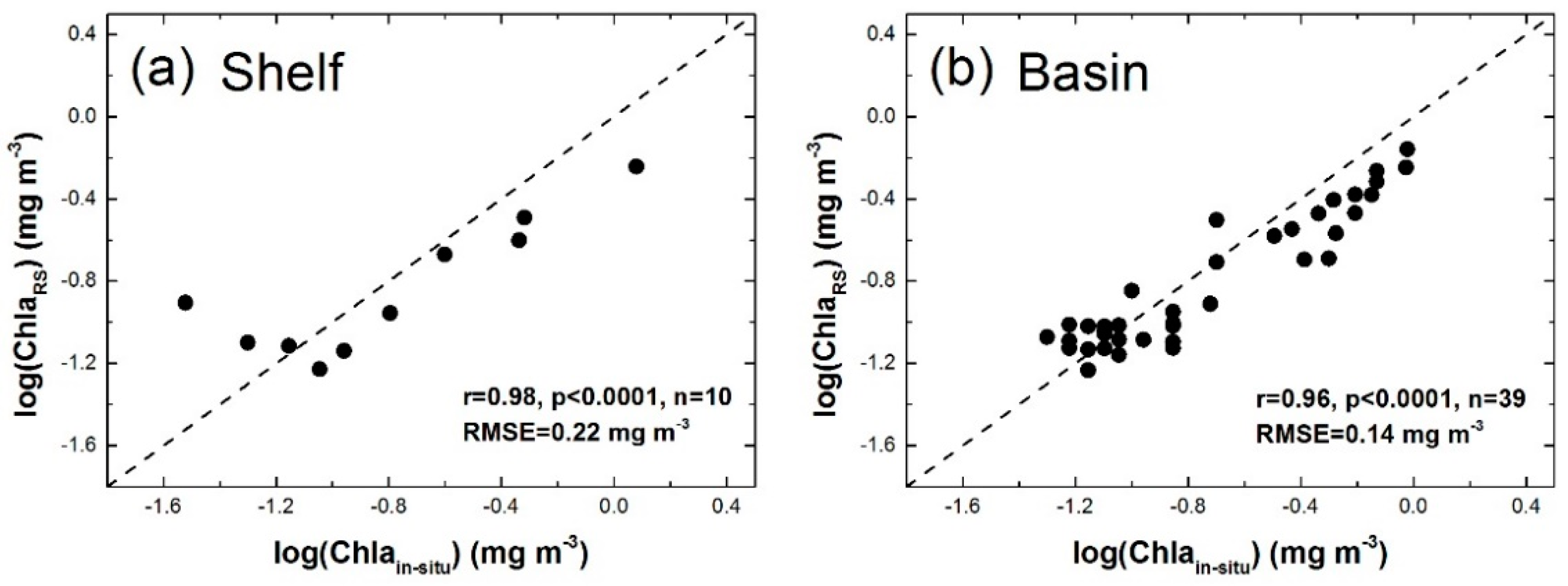
3.1.1. Applicability of VGPM Products in the NSCS

The applicability of VGPM algorithm for satellite retrieval of NPP in the NSCS has been demonstrated in previous studies [38,53,54]. Based on in situ NPP data from four surveys in the NSCS (including the shelf and basin areas), Hao et al. [53] observed a significant linear relationship between the VGPM-NPP and measured NPP values (r² = 0.79, n = 21, p < 0.0001). By collecting in situ NPP data (for the whole SCS in different seasons) from previous researches, Tan and Shi [54] also observed a good positive correlation (R = 0.705, n = 13, p < 0.0001) between VGPM-NPP and in situ NPP data. Xu et al. [55] conducted an inter-comparison of three satellite-derived NPP products estimated by standard VGPM, Eppley-VGPM [56], and CbPM models [57], and found the NPP products estimated by Eppley-VGPM and CbPM cannot reflect seasonal variation characteristics of NPP in the SCS, while the VGPM product can not only characterize the seasonal variation of NPP, but also its average value was closer to previous in situ NPP data than the other two algorithms, making it more suitable as the algorithm for satellite-derived NPP in the basin of SCS. VGPM-NPP was also used in modeling the long-term (1958–2009) variation of POC export flux and structure of the biological carbon pump in the SCS by a three-dimensional physical-biogeochemical coupled model (ROMS-CoSiNE) [31]. On the other hand, the results of Huang et al. [58] showed that CbPM-NCP (Carbon-based production model-net community production, equal to CbPM-NPP multiplied by an efficiency factor) were comparable to the oxygen mass balance estimated NCP in the central SCS, whereas the VGPM-NCP (equal to VGPM-NPP multiplied by the same efficiency factor as in calculating CbPM-NCP) were significantly lower. However, Huang et al. [58] also acknowledged that VGPM-NCP showed better performance than CbPM-NCP in representing the seasonal variation of NCP in the SCS.

As one of the main input parameters of the VGPM model, the accuracy of satellite-derived Chla is important for the applicability of VGPM products [52]. Figure 2 shows the comparison results between satellite-derived and in situ Chla (Chla_in-situ in Table A1) during the 2009–2011 cruises. To eliminate the effect of data missing by the cloud-mask of satellite data, three-day averaged satellite-derived Chla (3d-Chla_rs in Table A1) were used in the comparison. Generally, the satellite-derived Chla were significantly correlated with in situ Chla (around the 1:1 line), with the correlation coefficient value of 0.98 and 0.96 for the shelf and basin regions, respectively, although the satellite-derived Chla were slightly lower than the in situ results.

On-deck incubation of NPP is generally carried out around the same time with the ²³⁴Th sampling during 12 or 24 h. However, the residence time of ²³⁴Th is considered to be about 2–20 days [59]. This could introduce a mismatch in time scales between ²³⁴Th-derived POC export and the instantaneous NPP measured in situ [4]. That means the ²³⁴Th-derived POC export would reflect the NPP situation certain days earlier. According to Ho et al. [60], the residence time of ²³⁴Th in the upper 0–160 m layer was about 0.052 years (20 days) for the basin areas of NSCS. Liu et al. [37] also showed that the peak of POC export flux could lag the peak of NPP by about half a month in the basin of NSCS. Thus, 16-day composited satellite-derived NPP (hereafter, satellite-derived NPP) prior to the in situ measurement were used in subsequent analyses, same as the choice of Henson et al. [4] in their study on estimating POC export efficiency based on satellite-derived SST.

3.1.2. Seasonal Variation of POC Export Efficiency in Euphotic Layer of the NSCS

Based on the results of “analysis dataset”, significant seasonal and spatial variability of POC export efficiency in euphotic layer were observed in the NSCS (Figure 3, detailed data are listed in Table A1). In general, the high POC export efficiency was concentrated on the shelf area near the Pearl River plume-dominated region, and decreased toward the interior. High POC export efficiency also existed east of Hainan Island. POC export efficiency was the highest in autumn, followed by the values in spring and summer, and was the lowest in winter.

Seasonal mean EP_{in_situ}, EF_{in_situ} and NPP are shown in

Table 3. Seasonal mean values of NPP (mmol C·m⁻²·day⁻¹), EP_{in_situ} (mmol C·m⁻²·day⁻¹), and EF_{in_situ} (dimensionless) in different regions of the NSCS.

	Spring	Summer	Autumn	Winter
Shelf areas
NPP	22.05 ± 4.61	29.97 ± 17.47	50.18 ± 15.13	58.05 ± 10.63
EPin_situ	6.78 ± 5.22	10.74 ± 11.04	28.32 ± 22.49	16.18 ± 8.23
EFin_situ	0.28 ± 0.17	0.31 ± 0.14	0.53 ± 0.30	0.26 ± 0.10
Basin areas
NPP	22.04 ± 4.53	18.06 ± 2.38	31.56 ± 5.99	57.90 ± 15.13
EPin_situ	7.70 ± 2.61	4.35 ± 1.39	9.53 ± 2.99	4.52 ± 1.99
EFin_situ	0.36 ± 0.14	0.25 ± 0.09	0.34 ± 0.20	0.08 ± 0.04

. For the shelf areas, the values of NPP were the largest in winter, followed by relatively small values in autumn, and decreased significantly in spring and summer (by nearly two folds). However, both EP_{in_situ} and EF_{in_situ} reached their maxima in autumn. For the basin region, NPP was the largest in winter and the smallest in summer, while EP_{in_situ} was low in both winter and summer. Annual-averaged EF_{in_situ} values were 0.34 and 0.24 for the shelf and basin regions, respectively, consistent with the previous studies in the NSCS [25,29,35].

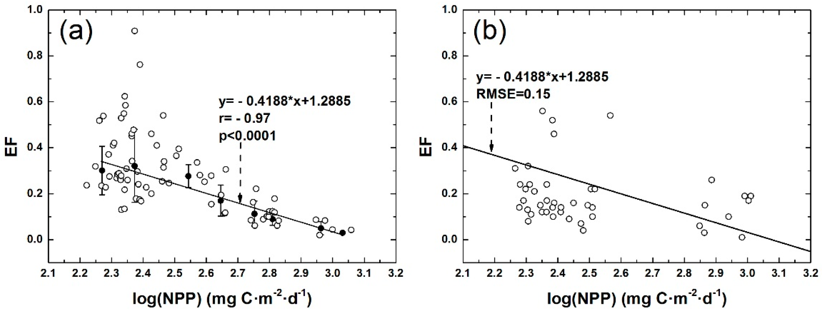
3.2. Correlation between POC Export Efficiency and NPP in Euphotic Layer of the NSCS

Based on the “analysis dataset”, EF_{in_situ} in euphotic layer tended to rise with the increase of NPP on the shelf areas (Figure 4a). However, in the basin areas, EF_{in_situ} and NPP showed a significant negative correlation (Figure 4b). While EF_{in_situ} was calculated from NPP, EF_{in_situ} and NPP were not independent variables and their relationships may overlook some of the variability in both NPP and EP_{in_situ} [61]. However, by checking the variation of EP_{in_situ} with NPP, we observed that EP_{in_situ} was positively correlated with NPP on the shelf areas (Figure 4c). For the basin areas, EP_{in_situ} tended to decrease slightly with the increase of NPP (Figure 4d). This suggests that the relationship between EF_{in_situ} and NPP in the NSCS was caused by the biogeochemical mechanism, not an artifact of plotting EP_{in_situ}/NPP versus NPP [61].

To further check the correlation of POC export efficiency and NPP in euphotic layer of the basin areas, we binned the EF_{in_situ} data based on the NPP rates with the ranges of 0–200, 200–300, 300–400, 400–500, 500–600, 600–700, 700–1000, and 1000–1300 mg C·m⁻²·day⁻¹ (Figure 5a). Averaged NPP and EF_{in_situ} values in each bin were used in the following analysis. Wider ranges were used at high NPP values to balance the distribution of data points. The relationship between logarithmic-NPP and POC export efficiency was robust (r = −0.97, p < 0.0001) in the basin areas. To evaluate the applicability of the linear fitting results shown in Figure 5a, POC export efficiency in euphotic layer was re-calculated by in situ POC export flux data from the “validation dataset” and corresponding satellite-derived NPP (see Table A2). The validation results also show an inverse relationship between POC export efficiency and NPP in euphotic layer for the basin areas, with the RMSE (root mean square error) value of 0.15 (Figure 5b).

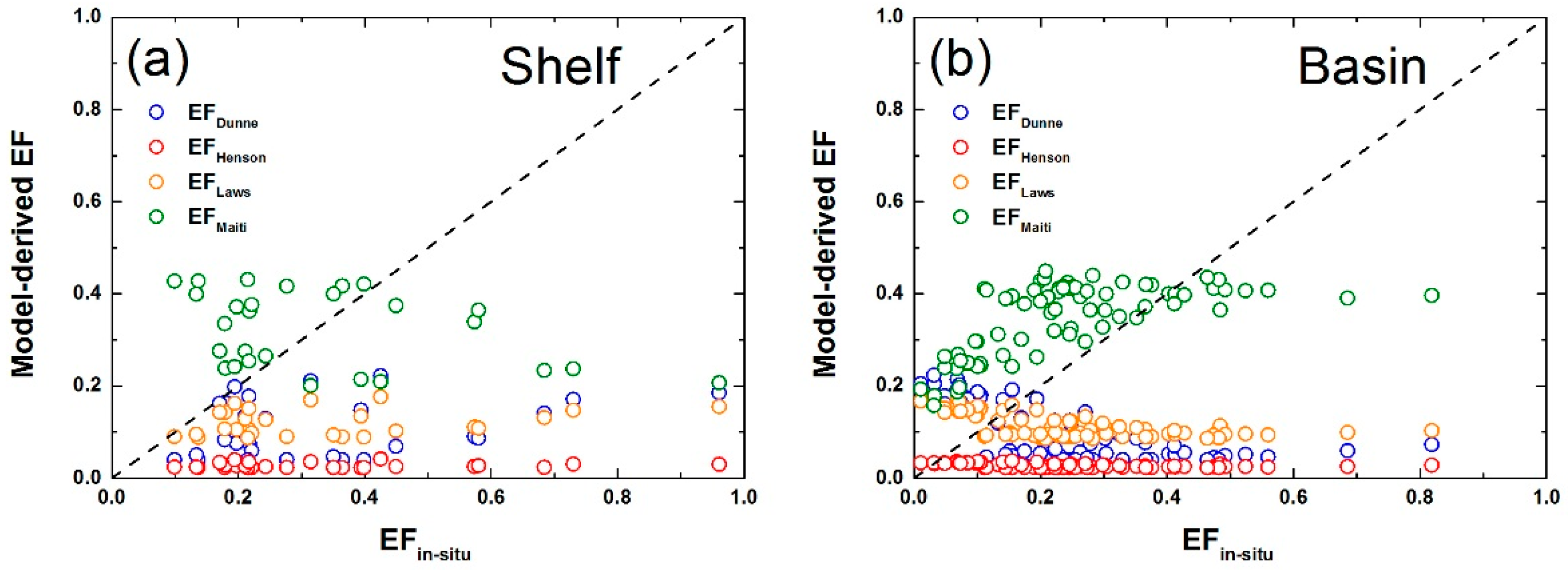
3.3. Comparison of Different Models of POC Export Efficiency

To contextualize within the field, we compared the calculated EF_{in_situ} (based on the “analysis dataset” and satellite-derived NPP) in the NSCS to the model-derived POC export efficiency results (Equations shown in Table 2, Figure 6). The NPP data used by all models were from the same VGPM-NPP dataset, which could eliminate the systematic deviation of model-derived EF variation trend with VGPM-NPP in Figure 6.

For the shelf areas (Figure 6a), the averaged EF_{in_situ}, EF_Dunne, EF_Henson, EF_Laws, and EF_Maiti were 0.34, 0.11, 0.03, 0.12, and 0.32, respectively, at the selected stations. Generally, EF_Dunne and EF_Laws showed similar trends, but their averaged relative deviations from EF_{in_situ} were high (60% and 53% for EF_Dunne and EF_Laws, respectively). EF_Maiti and EF_Henson had totally different trends from that of EF_{in_situ}, and they were not suitable to the shelf areas of the NSCS. Located in the tropical-subtropical area with high ocean temperature throughout the year (Figure 3), the solely SST-dependent model developed with the global data in Henson et al. [4] was invalid in the NSCS. As for the equation in Maiti et al. [16], the characteristic on the shelf of the NSCS was also different from that in the Southern Ocean.

For the basin areas (Figure 6b), the averaged EF_{in_situ}, EF_Dunne, EF_Henson, EF_Laws, and EF_Maiti were 0.25, 0.09, 0.03, 0.11, and 0.35, respectively, at the selected stations. Only EF_Maiti had similar trend and value as EF_{in_situ}, and the other three models showed significant disagreement in the basin of NSCS. Comparing with the large range of SST on the global ocean scale, the variation of SST in the NSCS is relatively small (Figure 3); thus, NPP is mainly controlled by the nutrient levels driven by monsoonal winds, the seasonal change of mixed layer depth, etc. [37]. According to recent studies, the temperature scaling for autotrophic processes is valid up to 40 °C, but the temperature dependency for zooplankton growth rate (thus, grazing rate) is only reasonable fit up to 24 °C, after which the temperature scaling breaks down and appears to flatten out due to decreased solubility of oxygen at higher temperature [62]. Since the SST in shelf and basin regions of NSCS are generally greater than 20 °C throughout the year (Figure 3), the algorithm considering only the influence of temperature may not well characterize the variation of POC export efficiency in euphotic layer of the NSCS. In fact, the relationship between SST and POC export efficiency was also unstable in the dataset of Henson et al. [4] and Laws et al. [15] when SST was higher than 24 °C.

4. Discussion

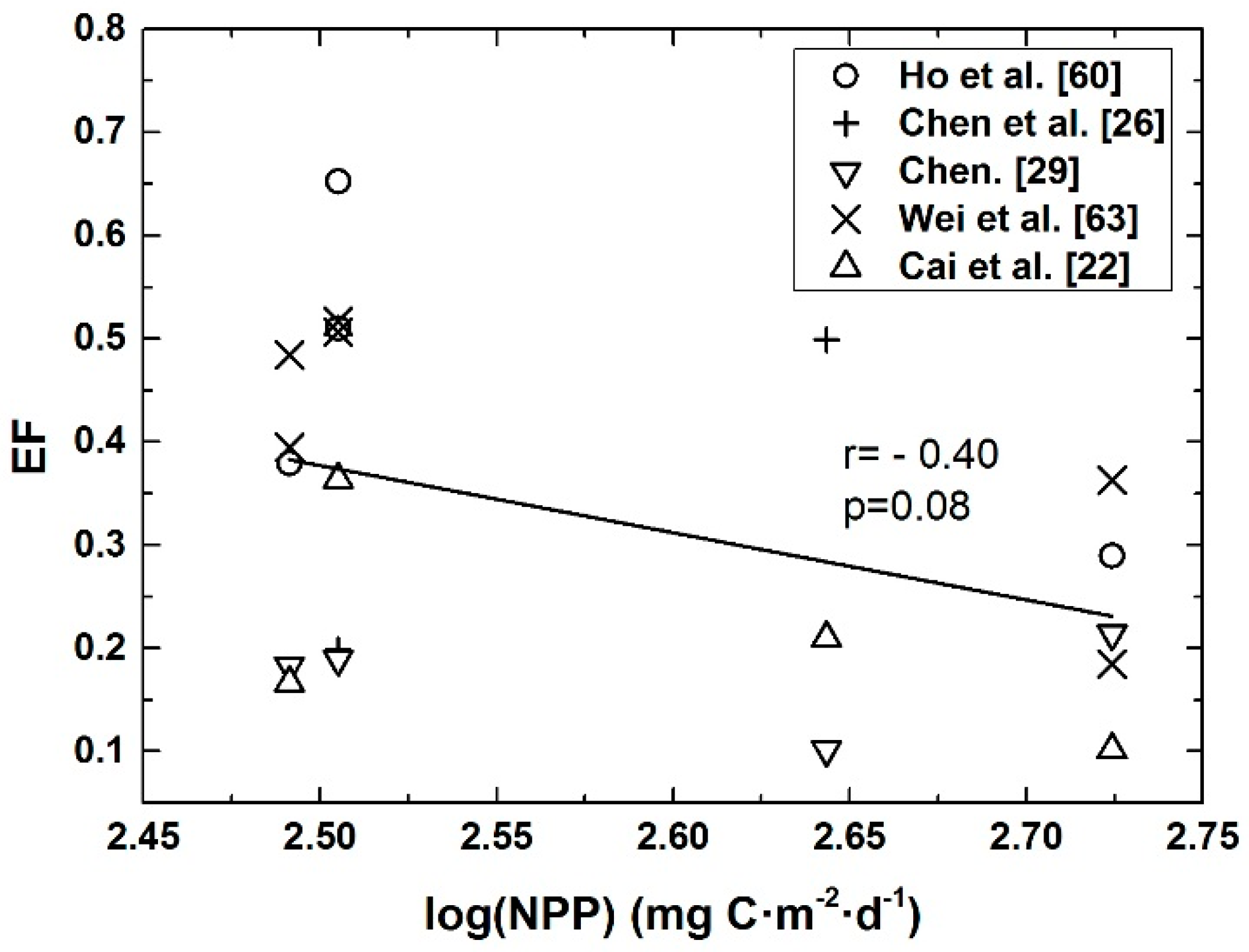
4.1. Seasonal Mean POC Export Efficiency and NPP in Euphotic Layer of the Basin Regions

Due to the long incubation periods necessary, we had less synchronous observation dataset of NPP and POC export flux in the NSCS. Therefore, we collected as many published data as possible to check the negative relationship between POC export efficiency and NPP in the basin. We used the in situ seasonal averaged NPP data from previous research [41], which included 30 sets of measurements from more than eight cruises in the NSCS (details can be found in

Table A3. Previous report of measured seasonal mean NPP in the basin of NSCS.

Season	Time	Number of Stations	NPP g C·m−2·day−1
Spring	March 2001	3	0.44 ± 0.30
	March 2002	4
Summer	27 June–4 July 2001	5	0.31 ± 0.14
	6–19 July 2003	4
	24 June–6 July 2004	2
Autumn	October 2001	1	0.32 ± 0.14
	October 2002	5
Winter	18–24 January 2003	1	0.53 ± 0.19
	10–22 February 2004	5

Note: Data are from Chen et al. [41].

), for the calculation of seasonal POC export efficiency in euphotic layer of basin regions. Individual field measurements of POC export flux in the basin of the NSCS were also gathered from previous researches (

Table 4. In situ POC export flux data collected from previous studies in the basin areas of NSCS.

Observation Period	POC Export Flux (mmol C·m−2·day−1)	Method	Reference
18–24 October 2006	17.4	Free floating sediment traps. Flux at 100 m.	Ho et al. [60]
12–19 January 2007	12.8
28 July–3 August 2007	9.8
21–30 October 2007	13.6
November 2002	5.3	234Th/238U disequilibrium. Flux at 100 m.	Chen et al. [26]
May 2001	18.3
29 April–11 May 2005	3.73	234Th/238U disequilibrium. Flux at 100 m.	Chen [29]
10–13 July 2004	4.73
19 September to 02 October 2004	5.06
18 February–1 March 2004	9.46
October 2006	17.29, 21.04, 8.60, 8.23	Fluxes were measured by floating sediment trap, 234Th, 210Po and 210Pb proxy respectively. Flux at 100 m.	Wei et al. [63]
January 2007	12.80, 9.51, 1.65, 8.69
July 2007	9.60, 11.43, 7.77, 21.22
October 2007	12.53, 10.52, 14.91, 16.10
June 2008	15.09, 13.54, 5.12, 7.04
December 2008	18.29, 13.72, 20.12, 11.98
30 April–24 May 2011	7.7	234Th/238U disequilibrium. Flux at 100 m.	Cai et al. [22]
18 July–16 August 2009	4.3
26 October–24 November 2010	9.7
6–30 January 2010	4.5

, only field data of POC export flux at 100-m depth were gathered). Although the inverse relationship between POC export efficiency and NPP in euphotic layer was not statistically significant on seasonal scale (Figure 7), these independent results also indicated that the POC export efficiency was not positively related to NPP in the basin areas of NSCS as suggested in the global models (Table 2).

4.2. Effect of Phytoplankton Community Structure

POC export variability is regulated by a combination of possesses and mechanisms, e.g., ultimate control by particle production and proximate control by the ability to generate sinking materials through phytoplankton size composition and temperature [14,64]. Generally, the larger the phytoplankton size is, the more efficient euphotic zone NPP is partitioned into export [7]. Larger cells, diatoms for example, have a greater chance of being associated with ballasting materials and the silica cell wall of diatoms is less labile, thus result in greater export efficiency [65]. Observation results also show that diatom-dominated phytoplankton communities in productive areas, such as oceans at high latitude and upwelling regions, have high POC export efficiency in euphotic layer; conversely, in lower latitude oligotrophic environments, where diatoms are largely absent, primary production is low and mostly regenerated, resulting in weak POC export efficiency in euphotic layer [65]. On the other hand, recent researches also revealed that pico-phytoplankton could dominate POC export through both direct aggregates and indirect grazing export of pico-phytoplankton-derived particles, referred to the studies in an ultra-oligotrophic lake on Vancouver Island, the equatorial Pacific Ocean and the Arabian Sea [66,67,68]. In the coastal and inter-shelf areas of the NSCS, it was reported that diatoms dominated the phytoplankton community structure in euphotic zone [22], especially in winter [36]. Considering the relatively fast sinking rate accompanied by diatoms and the shallow euphotic depth (about 50 m), micro-phytoplankton may play an important role in regulating the POC export efficiency on the shelf areas of the NSCS. For the basin regions, a weak but intriguing correlation (r ≈ 0.51, p < 0.0001) between POC export flux and the fraction of haptophytes and prasinophytesin (size typically < 5 µm) was reported in Cai et al. [22]. Observation of HPLC results during the 2009–2011 cruises also showed that, in the basin areas of NSCS, there was a significant positive correlation (p < 0.001) between POC export efficiency and the fraction of synechococcus and prochlorococcus (pico-phytoplankton) [69]. Phytoplankton community structure tended to have different effects on POC export efficiency in euphotic layer of the shelf and basin areas, although the specific regulatory mechanisms are not clear and need further investigation.

4.3. Factors in Driving the Inverse Relationship between POC Export Efficiency and NPP in Euphotic Layer of the Basin Regions

According to previous researches [16,17,61,70], the inverse relationship between NPP and POC export efficiency in euphotic layer may be caused by several factors, such as the differences in trophic structure, grazing intensity, recycling efficiency, high bacterial activity and increased DOC export in high NPP areas. Therefore, below we focus some regulation mechanisms that may cause the negative correlation between POC export efficiency and NPP in euphotic layer of the basin regions.

4.3.1. Effect of Zooplankton Grazing

According to the model-simulated results of Liu et al. [37], an average of 70% of the NPP in the euphotic layer of SCS could be removed by zooplankton grazing. Zooplankton grazing would result in POC either passing through the gut and being egested as fecal pellets, being respired as CO₂ or fragmenting into smaller particles through sloppy feeding [17,71]. In general, particle size is an important parameter that determines the POC export [72] as small-sized, slow sinking fecal debris produced by small meso-zooplankton may be reutilized either through remineralization or coprophagy within the euphotic layer, while large, fast sinking fecal pellets produced by large copepods significantly contribute to vertical carbon export [73,74]. Figure 8 shows the profile distributions of bbp442/bp442 in different seasons in the euphotic layer of the basin regions. Generally, the sea surface bbp442/bp442 values was small in winter and autumn, corresponding to the relatively larger fraction of micro-phytoplankton in surface water in winter and autumn than in the other seasons [36,75]. However, for the 100-m layer, the mean particle size was comparably smaller in winter than in the other seasons, with the largest mean value of bbp442/bp442 (0.0247). Thus, it is indicated that fecal pellets from zooplankton grazing appeared to be rapidly mineralized in euphotic zone, or the role of zooplankton grazing was more likely fragmenting large, fast sinking particles into smaller, slower sinking particles through sloppy feeding in winter for the basin areas of NSCS.

4.3.2. Effect of DOC Export in the Basin

In addition to the export of POC, NPP also results in the export of dissolved organic carbon (DOC) from the upper ocean [76]. A large DOC export flux in high NPP season would result in a low POC export efficiency. At HOT (Hawaii Ocean Time-Series) station, DOC production could be about 17–50% of total carbon fixation by phytoplankton [77]. Although the model-simulated results of Ma et al. [31] showed that the DOC export could be negligible in the basin of NSCS on annual average scale, with the net advection and diffusion DOC flux was about −0.02 mmol C·m⁻²·day⁻¹ (upward), Chen [29] observed that the DOC export could be relatively high in spring and winter. Accordingly, average net DOC diffusion export was about 0.91 mmol C·m⁻²·day⁻¹ (downward) in spring of NSCS, which may account for 30% of the POC export flux [29]. When in situ total organic carbon (TOC) inventory was used as an approximation of DOC, the seasonal variation of TOC inventory (23.80, 25.20 and 23.60 Tg in spring, autumn and winter, respectively [78]) in the basin of NSCS suggested a relatively strong TOC (hence DOC) export in winter. Given the lack of in situ DOC export data in the basin of NSCS, we attempted to summarize existing results in this section rather than quantitatively assess the impact of DOC export on the inverse relationship between NPP and POC export efficiency in the basin. More field DOC export flux observations are needed to quantify the role of DOC export in driving the inverse relationship between POC export efficiency and NPP in euphotic layer of the basin regions.

4.3.3. Seasonal Decoupling between Primary Production and POC Export

Before organic carbon produced by NPP is converted into sinking flux, it goes through many processes, such as aggregation of individual particles until reaching certain density or size before sinking, or grazing by zooplankton and subsequent excretion as fecal pellets [13]. These processes could lead to uncoupling between production and POC export, thus influencing the relationship between POC export efficiency and NPP. Unlike typical oceans in the tropics, the NPP and POC export in the NSCS are affected by monsoons with significant seasonal changes, and bloom occurs in the cold eddy or local upwelling northwest of Luzon in winter [36]. Cai et al. [22] reported that the seasonal average Chla stock was almost a factor of two higher in winter than in summer, while the seasonal average POC stock was only about 30% higher in winter than in summer in the basin of NSCS. Phytoplankton blooms might be developing in the NSCS basin during a winter survey and this may lead to an elevated NPP level, but not yet immediately enhanced POC export flux until the following spring, thus resulting in low POC export efficiency in winter in the basin of NSCS. Chen et al. [79] observed that grazed NPP of micro-zooplankton for the basin waters of the NSCS was smaller in winter (73% and 65% in summer and winter, respectively). According to previous research, the peak of POC export flux of euphotic layer could lag the peak of primary production by about half a month in the basin of NSCS [37]. In this research, we used the 16-day-composited satellite-derived NPP data prior to the ²³⁴Th sampling time, which can reduce the decoupling effect of NPP and POC export in the euphotic layer to some extent. However, due to the complex processes through the food web, more parameterizations need to be developed.

5. Conclusions

The carbon sequestration by biological carbon pump plays an important role in the global ocean carbon cycle. However, estimates of the strength and efficiency of the biological carbon pump remain poorly quantified due to the lack of in situ data. In this study, we utilized two datasets of seasonal ²³⁴Th-derived POC export flux at the euphotic depth and satellite-derived 16-day-composited NPP prior to the ²³⁴Th sampling time to examine the correlation between POC export efficiency and NPP in the euphotic layer of NSCS. The results revealed that, on the shelf areas of the NSCS, POC export efficiency in euphotic layer tended to rise with the increase of NPP, and the biological processes associated with large phytoplankton might play an important role in leading to this result. On the other hand, an inverse relationship between POC export efficiency and NPP was observed in euphotic layer of the basin areas. Grazing by zooplankton, DOC export and seasonal decoupling between NPP and POC export in euphotic layer might contribute to the inverse relationship. The global POC export efficiency models are inappropriate in the NSCS. More studies (i.e., POC sink rate, POC inventory, POC composition, etc.) are needed for understanding the evolution of carbon sequestration capacity of the NSCS in the context of climate change.

References

1. Falkowski, P.; Scholes, R.J.; Boyle, E.; Canadell, J.; Canfield, D.E.; Elser, J.; Gruber, N.; Hibbard, K.; Hogberg, P.; Linder, S. The global carbon cycle: A test of our knowledge of the earth as a system. Science 2000, 290, 291–296. [Google Scholar] [CrossRef] [PubMed]
2. DeVries, T.; Primeau, F.; Deutsch, C. The sequestration efficiency of the biological pump. Geophys. Res. Lett. 2012, 39, L13601. [Google Scholar] [CrossRef]
3. Ducklow, H.W.; Steinberg, D.K.; Buesseler, K.O. Upper ocean carbon export and the biological pump. Oceanography 2001, 14, 50–58. [Google Scholar] [CrossRef]
4. Henson, S.A.; Sanders, R.; Madsen, E.; Morris, P.J.; Moigne, F.L.; Quartly, G.D. A reduced estimate of the strength of the ocean’s biological carbon pump. Geophys. Res. Lett. 2011, 38, L04606. [Google Scholar] [CrossRef]
5. Tsunogai, S.; Watanabe, S.; Sato, T. Is there a “continental shelf pump” for the absorption of atmospheric CO2? Tellus B 1999, 51, 701–712. [Google Scholar] [CrossRef]
6. Boyd, P.W.; Trull, T.W. Understanding the export of biogenic particles in oceanic waters: Is there consensus? Prog. Oceanogr. 2007, 72, 276–312. [Google Scholar] [CrossRef]
7. Siegel, D.A.; Buesseler, K.O.; Doney, S.C.; Sailley, S.F.; Behrenfeld, M.J.; Boyd, P.W. Global assessment of ocean carbon export by combining satellite observations and food-web models. Glob. Biogeochem. Cycles 2014, 28, 181–196. [Google Scholar] [CrossRef] [Green Version]
8. Maiti, K.; Bosu, S.; D’Sa, E.J.; Adhikari, P.L.; Sutor, M.; Longnecker, K. Export fluxes in northern gulf of mexico-comparative evaluation of direct, indirect and satellite-based estimates. Mar. Chem. 2016, 184, 60–77. [Google Scholar] [CrossRef]
9. Bopp, L.; Monfray, P.; Aumont, O.; Dufresne, J.L.; Le Treut, H.; Madec, G.; Terray, L.; Orr, J.C. Potential impact of climate change on marine export production. Glob. Biogeochem. Cycles 2001, 15, 81–99. [Google Scholar] [CrossRef] [Green Version]
10. Gregg, W.W.; Conkright, M.E.; Ginoux, P.; Oreilly, J.E.; Casey, N.W. Ocean primary production and climate: Global decadal changes. Geophys. Res. Lett. 2003, 30, 1809:1–1809:4. [Google Scholar] [CrossRef]
11. Hoegh-Guldberg, O.; Bruno, J.F. The impact of climate change on the world’s marine ecosystems. Science 2010, 328, 1523–1528. [Google Scholar] [CrossRef] [PubMed]
12. Steinacher, M.; Joos, F.; Frolicher, T.L.; Bopp, L.; Cadule, P.; Cocco, V.; Doney, S.C.; Gehlen, M.; Lindsay, K.; Moore, J.K. Projected 21st century decrease in marine productivity: A multi-model analysis. Biogeosciences 2010, 7, 979–1005. [Google Scholar] [CrossRef] [Green Version]
13. Henson, S.A.; Yool, A.; Sanders, R.J. Variability in efficiency of particulate organic carbon export: A model study. Glob. Biogeochem. Cycles 2015, 29, 33–45. [Google Scholar] [CrossRef] [Green Version]
14. Dunne, J.P.; Armstrong, R.A.; Gnanadesikan, A.; Sarmiento, J.L. Empirical and mechanistic models for the particle export ratio. Glob. Biogeochem. Cycles 2005, 19. [Google Scholar] [CrossRef] [Green Version]
15. Laws, E.A.; Dsa, E.J.; Naik, P. Simple equations to estimate ratios of new or export production to total production from satellite-derived estimates of sea surface temperature and primary production. Limnol. Oceanogr. Methods 2011, 9, 593–601. [Google Scholar] [CrossRef] [Green Version]
16. Maiti, K.; Charette, M.A.; Buesseler, K.O.; Kahru, M. An inverse relationship between production and export efficiency in the Southern Ocean. Geophys. Res. Lett. 2013, 40, 1557–1561. [Google Scholar] [CrossRef] [Green Version]
17. Cavan, E.; Henson, S.A.; Belcher, A.; Sanders, R.J. Role of zooplankton in determining the efficiency of the biological carbon pump. Biogeosciences 2017, 14, 177–186. [Google Scholar] [CrossRef]
18. Chen, C.; Shiah, F.K.; Chung, S.W.; Liu, K.K. Winter phytoplankton blooms in the shallow mixed layer of the south china sea enhanced by upwelling. J. Mar. Syst. 2006, 59, 97–110. [Google Scholar] [CrossRef]
19. Hu, S.; Cao, W.; Wang, G.; Xu, Z.; Zhao, W.; Lin, J.; Zhou, W.; Yao, L. Empirical ocean color algorithm for estimating particulate organic carbon in the south china sea. Chin. J. Oceanol. Limnol. 2015, 33, 764–778. [Google Scholar] [CrossRef]
20. Chen, X.; Pan, D.; Bai, Y.; He, X.; Chen, C.T.A.; Kang, Y.; Tao, B. Estimation of typhoon-enhanced primary production in the south china sea: A comparison with the Western North Pacific. Cont. Shelf Res. 2015, 111, 286–293. [Google Scholar] [CrossRef]
21. He, X.; Xu, D.; Bai, Y.; Pan, D.; Chen, C.T.A.; Chen, X.; Gong, F. Eddy-entrained Pearl River plume into the oligotrophic basin of the South China Sea. Cont. Shelf Res. 2016, 124, 117–124. [Google Scholar] [CrossRef]
22. Cai, P.; Zhao, D.; Wang, L.; Huang, B.; Dai, M. Role of particle stock and phytoplankton community structure in regulating particulate organic carbon export in a large marginal sea. J. Geophys. Res. Oceans 2015, 120, 2063–2095. [Google Scholar] [CrossRef]
23. Liu, G.; Chai, F. Seasonal and interannual variability of primary and export production in the south china sea: A three-dimensional physical–biogeochemical model study. ICES J. Mar. Sci. 2008, 66, 420–431. [Google Scholar] [CrossRef]
24. Cai, P.; Chen, W.; Dai, M.; Wan, Z.; Wang, D.; Li, Q.; Tang, T.; Lv, D. A high-resolution study of particle export in the southern south china sea based on 234th:238u disequilibrium. J. Geophys. Res. 2008, 113, C04019. [Google Scholar] [CrossRef]
25. Cai, P.; Huang, Y.; Chen, M.; Liu, G.; Qiu, Y. New production in the South China Sea. Sci. China Ser. D Earth Sci. 2002, 45, 103–109. [Google Scholar] [CrossRef]
26. Chen, W.; Cai, P.; Dai, M.; Wei, J. 234th/238u disequilibrium and particulate organic carbon export in the northern South China Sea. J. Oceanogr. 2008, 64, 417–428. [Google Scholar] [CrossRef]
27. Ma, H.; Zeng, Z.; He, J.; Chen, L.; Yin, M.; Zeng, S.; Zeng, W. Vertical flux of particulate organic carbon in the central South China Sea estimated from 234th-238u disequilibria. Chin. J. Oceanol. Limnol. 2008, 26, 480–485. [Google Scholar] [CrossRef]
28. Lui, H.; Chen, K.; Chen, C.T.A.; Wang, B.; Lin, H.; Ho, S.; Tseng, C.; Yang, Y.; Chan, J. Physical forcing-driven productivity and sediment flux to the deep basin of northern South China Sea: A decadal time series study. Sustainability 2018, 10, 971. [Google Scholar] [CrossRef]
29. Chen, W. On the Export Fluxes, Seasonality and Controls of Particulate Organic Carbon in the Northern South China Sea. Ph.D. Thesis, Xiamen University, Xiamen, China, 2008. [Google Scholar]
30. Hung, J.J.; Wang, S.M.; Chen, Y.L. Biogeochemical controls on distributions and fluxes of dissolved and particulate organic carbon in the northern South China Sea. Deep Sea Res Part 2 Top. Stud. Oceanogr. 2007, 54, 1486–1503. [Google Scholar] [CrossRef]
31. Ma, W.; Chai, F.; Xiu, P.; Xue, H.; Tian, J. Simulation of export production and biological pump structure in the South China Sea. Geo-Mar. Lett. 2014, 34, 541–554. [Google Scholar] [CrossRef]
32. Hu, J.; Kawamura, H.; Hong, H.; Qi, Y. A review on the currents in the South China Sea: Seasonal circulation, South China Sea warm current and Kuroshio intrusion. J. Oceanogr. 2000, 56, 607–624. [Google Scholar] [CrossRef]
33. Shaw, P.; Chao, S. Surface circulation in the South China Sea. Deep Sea Res. Part 1 Oceanogr. Res. Pap. 1994, 41, 1663–1683. [Google Scholar] [CrossRef]
34. Chen, C.T.A.; Wang, S.; Lu, X.X.; Zhang, S.; Lui, H.; Tseng, H.; Wang, B.; Huang, H. Hydrogeochemistry and greenhouse gases of the Pearl River, its estuary and beyond. Quat. Int. 2008, 186, 79–90. [Google Scholar] [CrossRef]
35. Chen, Y. Spatial and seasonal variations of nitrate-based new production and primary production in the South China Sea. Deep Sea Res. Part 1 Oceanogr. Res. Pap. 2005, 52, 319–340. [Google Scholar] [CrossRef]
36. Ning, X.; Chai, F.; Xue, H.; Cai, Y.; Liu, C.; Shi, J. Physical-biological oceanographic coupling influencing phytoplankton and primary production in the South China Sea. J. Geophys. Res. 2004, 109, C10005. [Google Scholar] [CrossRef]
37. Liu, K.K.; Chao, S.Y.; Shaw, P.T.; Gong, G.C.; Chen, C.C.; Tang, T.Y. Monsoon-forced chlorophyll distribution and primary production in the South China Sea: Observations and a numerical study. Deep Sea Res. Part 1 Oceanogr. Res. Pap. 2002, 49, 1387–1412. [Google Scholar] [CrossRef]
38. Zhao, H.; Tang, D.; Wang, Y. Comparison of phytoplankton blooms triggered by two typhoons with different intensities and translation speeds in the South China Sea. Mar. Ecol. Prog. Ser. 2008, 365, 57–65. [Google Scholar] [CrossRef] [Green Version]
39. Xian, T.; Sun, L.; Yang, Y.; Fu, Y. Monsoon and eddy forcing of chlorophyll-a variation in the northeast South China Sea. Int. J. Remote Sens. 2012, 33, 7431–7443. [Google Scholar] [CrossRef]
40. Pan, X.; Wong, G.T.; Shiah, F.-K.; Ho, T.-Y. Enhancement of biological productivity by internal waves: Observations in the summertime in the northern South China Sea. J. Oceanogr. 2012, 68, 427–437. [Google Scholar] [CrossRef]
41. Chen, Y.; Chen, H. Seasonal dynamics of primary and new production in the northern South China Sea: The significance of river discharge and nutrient advection. Deep Sea Res. Part 1 Oceanogr. Res. Pap. 2006, 53, 971–986. [Google Scholar] [CrossRef]
42. Wu, Y.; Cheng, G.-S. Seasonal and inter-annual variations of the mixed layer depth in the South China Sea. Mar. Forcasts 2013, 30, 9–17. [Google Scholar]
43. Shang, S.; Lee, Z.; Wei, G. Characterization of modis-derived euphotic zone depth: Results for the china sea. Remote Sens. Environ. 2011, 115, 180–186. [Google Scholar] [CrossRef]
44. He, X.; Pan, D.; Bai, Y.; Wang, T.; Chen, C.-T.A.; Zhu, Q.; Hao, Z.; Gong, F. Recent changes of global ocean transparency observed by seawifs. Cont. Shelf Res. 2017, 143, 159–166. [Google Scholar] [CrossRef]
45. Mueller, J.L.; Fargion, G.S.; McClain, C.R.; Pegau, S.; Zanefeld, J.; Mitchell, B.G.; Kahru, M.; Wieland, J.; Stramska, M. Ocean Optics Protocols for Satellite Ocean Color Sensor Validation, Revision 4, Volume IV: Inherent Optical Properties: Instruments, Characterizations, Field Measurements and Data Analysis Protocols. Available online: https://oceancolor.gsfc.nasa.gov/docs/technical/protocols_ver4_voliv.pdf (accessed on 10 September 2015).
46. Morel, A. Optical properties of pure water and pure sea water. Opt. Asp. Oceanogr. 1974, 1, 1–24. [Google Scholar]
47. Reynolds, R.A.; Stramski, D.; Wright, V.M.; Woźniak, S.B. Measurements and characterization of particle size distributions in coastal waters. J. Geophys. Res. 2010, 115. [Google Scholar] [CrossRef] [Green Version]
48. Stramski, D.; Boss, E.; Bogucki, D.; Voss, K.J. The role of seawater constituents in light backscattering in the ocean. Prog. Oceanogr. 2004, 61, 27–56. [Google Scholar] [CrossRef]
49. Ulloa, O.; Sathyendranath, S.; Platt, T. Effect of the particle-size distribution on the backscattering ratio in seawater. Appl. Opt. 1994, 33, 7070–7077. [Google Scholar] [CrossRef] [PubMed]
50. Globcolour. Globcolour Product User Guide. Available online: http://hermes.acri.fr (accessed on 17 July 2017).
51. Morel, A.; Berthon, J.F. Surface pigments, algal biomass profiles, and potential production of the euphotic layer: Relationships reinvestigated in view of remote-sensing applications. Limnol. Oceanogr. 1989, 34, 1545–1562. [Google Scholar] [CrossRef] [Green Version]
52. Behrenfeld, M.J.; Falkowski, P.G. Photosynthetic rates derived from satellite-based chlorophyll concentration. Limnol. Oceanogr. 1997, 42, 1–20. [Google Scholar] [CrossRef] [Green Version]
53. Hao, J.; Ning, X.; Liu, C.; Cai, Y.; Cai, F. Satellite and in situ observations of primary production in the northern South China Sea. Acta Oceanol. Sin. 2007, 29, 58–68. [Google Scholar]
54. Tan, S.C.; Shi, G.Y. Spatiotemporal variability of satellite-derived primary production in the South China Sea, 1998–2006. J. Geophys. Res. 2009, 114, G03015. [Google Scholar] [CrossRef]
55. Xu, H.; Zhou, W.; Li, A.; Ji, S. Similarities and differences of oceanic primary productivity product estimated by three models based on modis for the open South China Sea. In Proceedings of the 4th International Conference on Geo-Informatics in Resource Management and Sustainable Ecosystems, Hong Kong, China, 18–20 November 2016; pp. 328–336. [Google Scholar]
56. Antoine, D.; Morel, A. Oceanic primary production: 1. Adaptation of a spectral light-photosynthesis model in view of application to satellite chlorophyll observations. Glob. Biogeochem. Cycles 1996, 10, 43–55. [Google Scholar] [CrossRef]
57. Behrenfeld, M.J.; Boss, E.; Siegel, D.A.; Shea, D.M. Carbon-based ocean productivity and phytoplankton physiology from space. Glob. Biogeochem. Cycles 2005, 19. [Google Scholar] [CrossRef] [Green Version]
58. Huang, Y.; Yang, B.; Chen, B.; Qiu, G.; Wang, H.; Huang, B. Net community production in the South China Sea basin estimated from in situ O2 measurements on an argo profiling float. Deep Sea Res. Part 1 Oceanogr. Res. Pap. 2018, 131, 54–61. [Google Scholar] [CrossRef]
59. Coale, K.H.; Bruland, K.W. 234th:238u disequilibria within the Californian current. Limnol. Oceanogr. 1985, 30, 22–33. [Google Scholar] [CrossRef]
60. Ho, T.; Chou, W.; Wei, C.; Lin, F.; Wong, G.T.F.; Line, H. Trace metal cycling in the surface water of the South China Sea: Vertical fluxes, composition, and sources. Limnol. Oceanogr. 2010, 55, 1807–1820. [Google Scholar] [CrossRef] [Green Version]
61. Moigne, F.A.C.L.; Henson, S.A.; Cavan, E.; Georges, C.; Pabortsava, K.; Achterberg, E.P.; Ceballosromero, E.; Zubkov, M.V.; Sanders, R. What causes the inverse relationship between primary production and export efficiency in the Southern Ocean. Geophys. Res. Lett. 2016, 43, 4457–4466. [Google Scholar] [CrossRef]
62. Cael, B.B.; Follows, M.J. On the temperature dependence of oceanic export efficiency. Geophys. Res. Lett. 2016, 43, 5170–5175. [Google Scholar] [CrossRef] [Green Version]
63. Wei, C.L.; Lin, S.Y.; Sheu, D.D.; Chou, W.; Yi, M.C.; Santschi, P.H.; Wen, L.S. Particle-reactive radionuclides (234th, 210pb, 210po) as tracers for the estimation of export production in the South China Sea. Biogeosciences 2011, 8, 3793–3808. [Google Scholar] [CrossRef]
64. Basu, S.; Mackey, K.R.M. Phytoplankton as key mediators of the biological carbon pump: Their responses to a changing climate. Sustainability 2018, 10, 869. [Google Scholar] [CrossRef]
65. Mouw, C.B.; Barnett, A.; McKinley, G.A.; Gloege, L.; Pilcher, D. Phytoplankton size impact on export flux in the global ocean. Glob. Biogeochem. Cycles 2016, 30, 1542–1562. [Google Scholar] [CrossRef]
66. Barber, R.T. Picoplankton do some heavy lifting. Science 2007, 315, 777–778. [Google Scholar] [CrossRef] [PubMed]
67. Klut, M.E.; Stockner, J.G. Picoplankton associations in an ultra-oligotrophic lake on Vancouver Island, British Columbia. Can. J. Fish. Aquat. Sci. 1991, 48, 1092–1099. [Google Scholar] [CrossRef]
68. Richardson, T.L.; Jackson, G.A. Small phytoplankton and carbon export from the surface ocean. Science 2007, 315, 838–840. [Google Scholar] [CrossRef] [PubMed]
69. Wang, L. The Spatio-Temporal Variation of Phytoplankton Community Structure and Its Responses to Mesoscale Physical Processes in the South China Sea. Ph.D. Thesis, Xiamen Univerisity, Xiamen, China, 2012. [Google Scholar]
70. Hansell, D.A.; Carlson, C.A.; Repeta, D.J.; Schlitzer, R. Dissolved organic matter in the ocean: A controversy stimulates new insights. Oceanography 2009, 22, 202–211. [Google Scholar] [CrossRef]
71. Lampitt, R.S.; Noji, T.T.; Von Bodungen, B. What happens to zooplankton faecal pellets? Implications for material flux. Mar. Biol. 1990, 104, 15–23. [Google Scholar] [CrossRef]
72. Berelson, W.M. Particle settling rates increase with depth in the ocean. Deep Sea Res. Part 2 Top. Stud. Oceanogr. 2001, 49, 237–251. [Google Scholar] [CrossRef]
73. Chen, M.; Liu, H.; Song, S.; Sun, J. Size-fractionated mesozooplankton biomass and grazing impact on phytoplankton in northern South China Sea during four seasons. Deep Sea Res. Part 2 Top. Stud. Oceanogr. 2015, 117, 108–118. [Google Scholar] [CrossRef]
74. Landry, M.R.; Lorenzen, C.J.; Peterson, W.K. Mesozooplankton grazing in the Southern California bight. Ii. Grazing impact and particulate flux. Mar. Ecol. Prog. Ser. 1994, 115, 73–85. [Google Scholar] [CrossRef]
75. Ho, T.; Pan, X.; Yang, H.-H.; Wong, G.T.F.; Shiah, F.-K. Controls on temporal and spatial variations of phytoplankton pigment distribution in the Northern South China Sea. Deep Sea Res. Part 2 Top. Stud. Oceanogr. 2015, 117, 65–85. [Google Scholar] [CrossRef]
76. Zheng, H.; Yan, Z.; Chen, J.; Jin, H.; Chen, C.; Liu, M.; Yan, Z.; Ji, Z. Seasonal variations of dissolved organic matter in the east china sea using eem-parafac and implications for carbon and nutrient cycling. Sustainability 2018, 10, 1444. [Google Scholar] [CrossRef]
77. Karl, D.M.; Hebel, D.V.; Bjorkman, K.M.; Letelier, R.M. The role of dissolved organic matter release in the productivity of the oligotrophic North Pacific Ocean. Limnol. Oceanogr. 1998, 43, 1270–1286. [Google Scholar] [CrossRef] [Green Version]
78. Wu, K.; Dai, M.; Chen, J.; Meng, F.; Li, X.; Liu, Z.; Du, C.; Gan, J. Dissolved organic carbon in the South China Sea and its exchange with the Western Pacific Ocean. Deep Sea Res. Part 2 Top. Stud. Oceanogr. 2015, 122, 41–51. [Google Scholar] [CrossRef]
79. Chen, B.; Zheng, L.; Huang, B.; Song, S.; Liu, H. Seasonal and spatial comparisons of phytoplankton growth and mortality rates due to microzooplankton grazing in the northern South China Sea. Biogeosciences 2013, 10, 2775–2785. [Google Scholar] [CrossRef]
Figure 1. Spatial distribution of sampling stations. Diamonds and boxes symbols show the POC export flux stations in analysis dataset (2009–2011 cruises) and validation dataset (2004–2005 cruises), respectively. Crosses symbols indicate the IOP stations during the 2009–2011 cruises. Black contours indicate bathymetry at 50 and 200 m, respectively. The background is climatology monthly mean seawater transparency in NSCS from 2003 to 2016 (only results of the corresponding months during 2009–2011 cruises are shown). Seawater transparency was retrieved by MODIS-derived reflectance, total absorption coefficient and particulate backscattering coefficient at 443 nm based on the semi-analytic algorithm of He et al. [44].
Sustainability 10 03634 g001
Figure 2. Comparison results between three-day satellite-derived Chla (ChlaRS) and in situ Chla (Chlain-situ) on the shelf (a) and basin (b) of the NSCS, respectively, during the 2009–2011 cruises.
Sustainability 10 03634 g002
Figure 3. Spatiotemporal distributions of POC export efficiency in euphotic layer of the NSCS in four seasons (Table A1). The backgrounds are monthly averaged SST from MODIS/Aqua during the 2009–2011 cruises. Two black lines indicate the 50- and 200-m isobaths which are used to divide the coastal, shelf and basin areas in the NSCS.
Sustainability 10 03634 g003
Figure 4. Correlations between POC export efficiency (EFin_situ) and NPP in euphotic layer (top), and between POC export flux (EPin_situ) and NPP (bottom): (a,c) for shelf areas; and (b,d) for basin region. Black lines are the linear fitting results.
Sustainability 10 03634 g004
Figure 5. Relationship between NPP and POC export efficiency (EF) in euphotic layer of the basin regions: (a) results based on the “analysis dataset” (see Table A1); and (b) results from the “validation dataset” (see Table A2). Open circles are original matching points, and black dots are the averaged data in different NPP bins. Solid line is the regression result in Figure 5a. Error bars show the standard errors of the mean.
Sustainability 10 03634 g005
Figure 6. Comparison between EFin_situ and model-derived EF on the shelf (a) and basin (b) regions of NSCS. Equations of models are shown in Table 2, with the parameter values given in Table A1. Dashed lines are the 1:1 lines.
Sustainability 10 03634 g006
Figure 7. Seasonal variation of POC export efficiency along with NPP in euphotic layer of the basin areas. Black line is the linear fitting result. In situ POC export flux data were collected from previous studies in the basin areas of NSCS (Table 4) while in situ NPP data were from Chen et al. [41] (Table A3).
Sustainability 10 03634 g007
Figure 8. Profile distributions of particulate backscattering ratio at 442 nm (bbp442/bp442) in four seasons for the basin areas of NSCS. Black lines are the linear fitting results. See Figure 1 for the locations of optical stations. Different colors indicate profile data for different sampling stations.
Sustainability 10 03634 g008