A Regionalized Study on the Spatial-Temporal Changes of Grassland Cover in the Three-River Headwaters Region from 2000 to 2016


Abstract
1. Introduction
2. Study Area and Materials
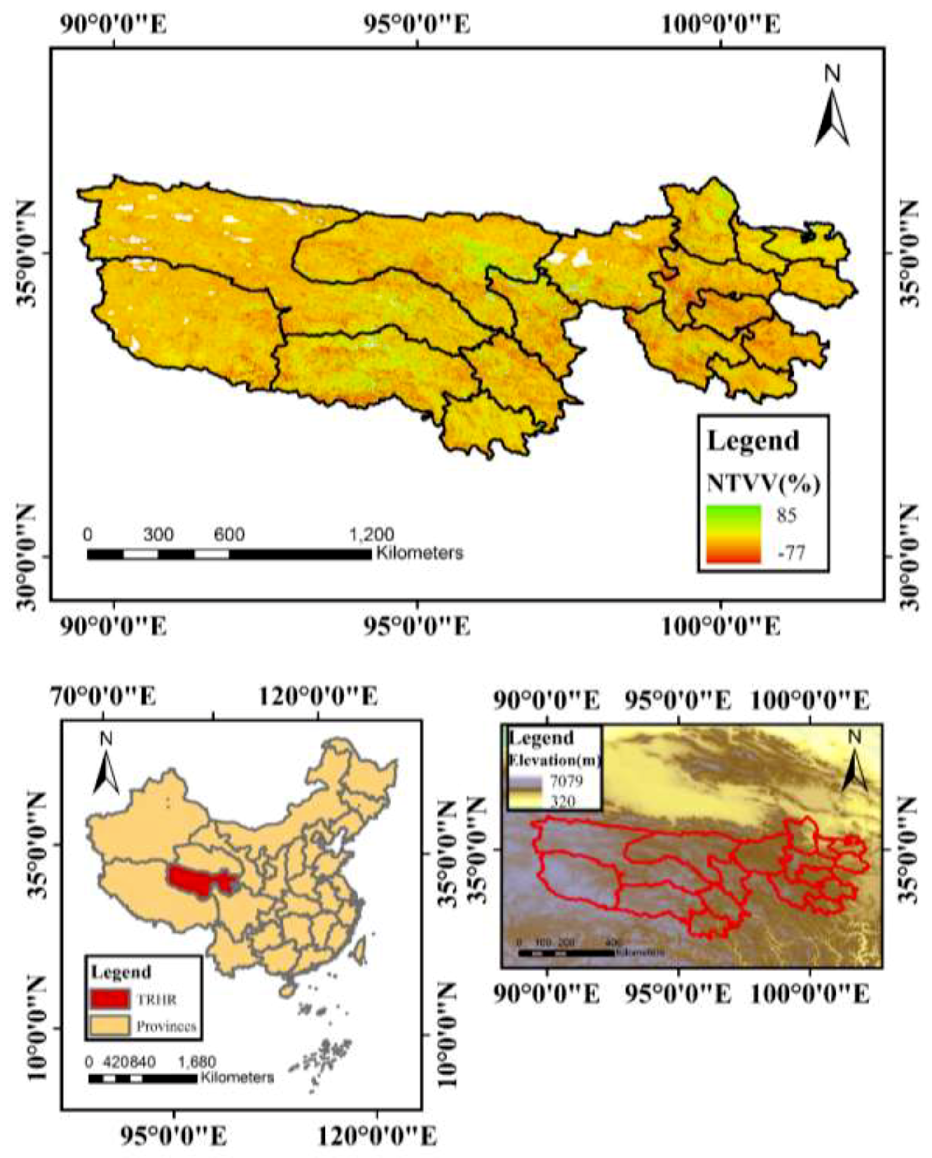
2.1. Study Area
2.2. Data Source and Preprocessing
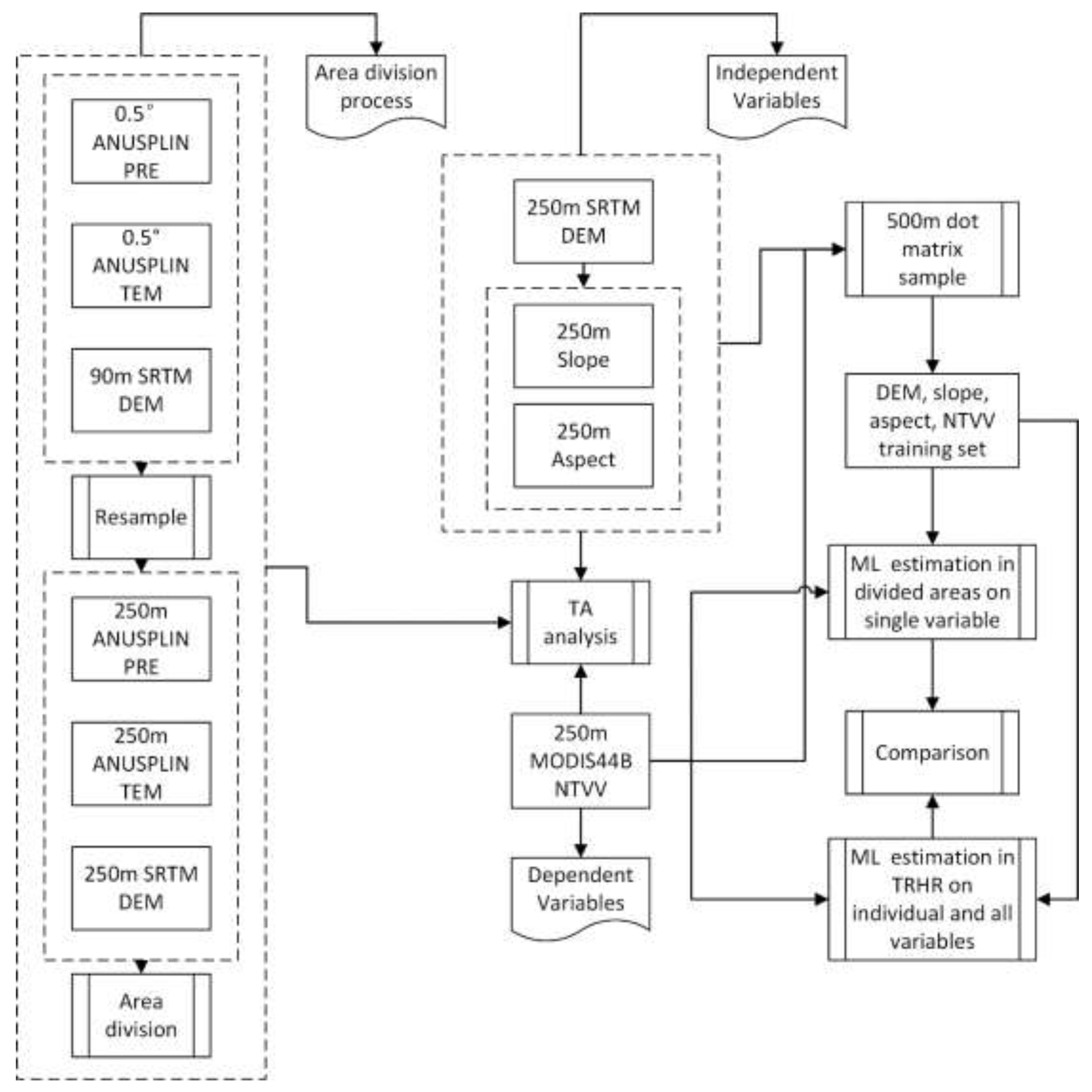
3. Methods
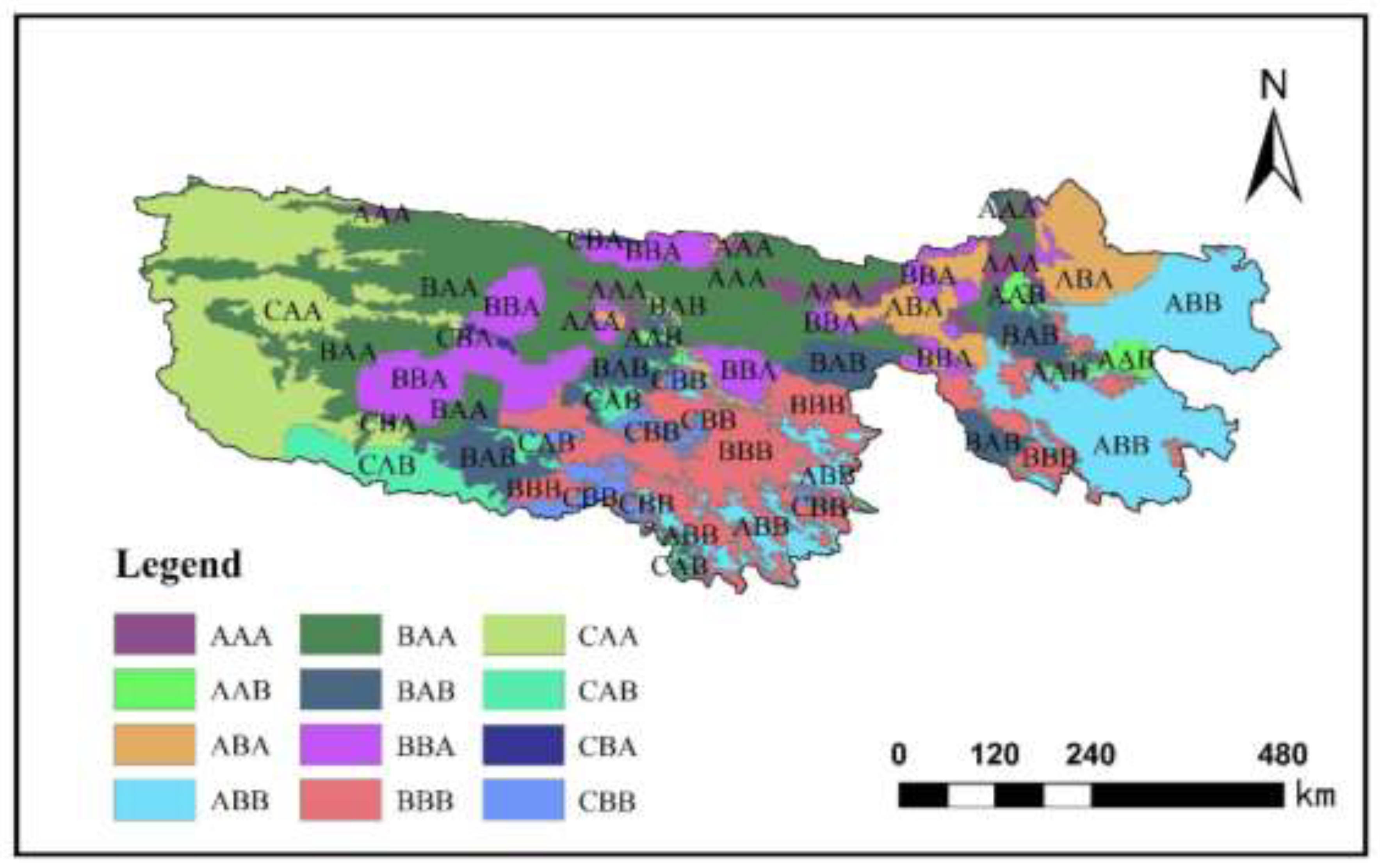
3.1. Area Division Process
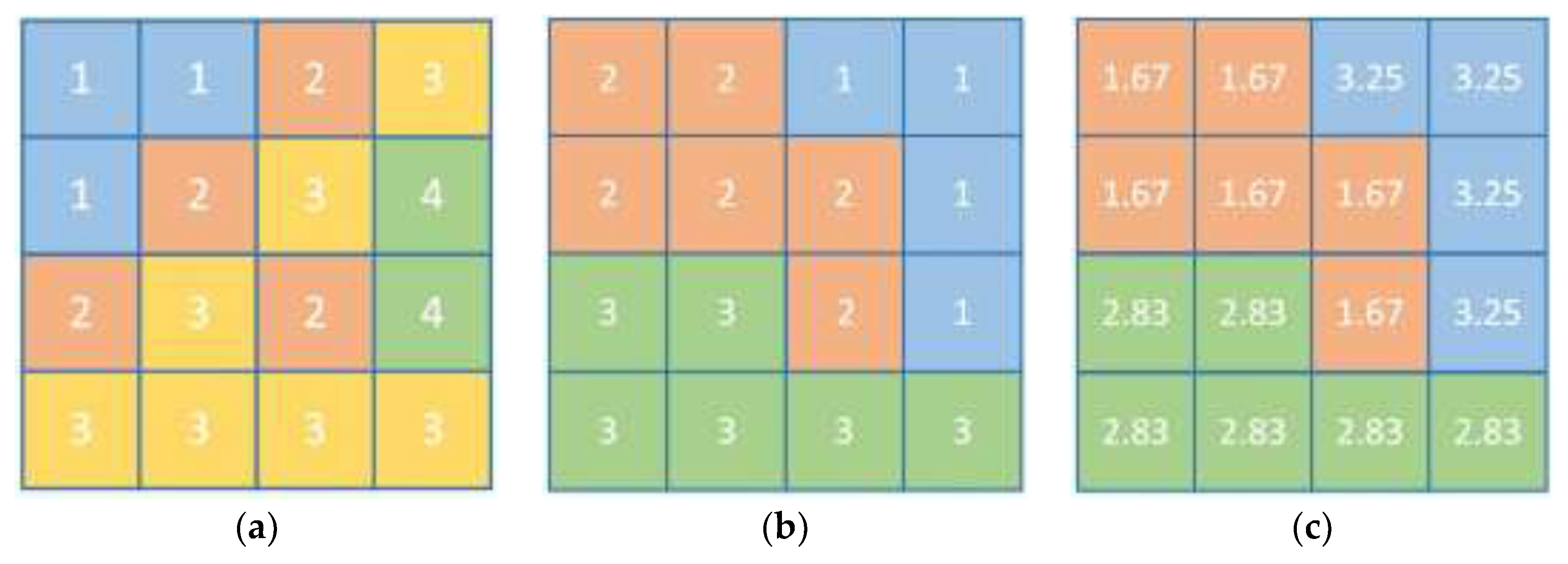
3.2. Tabulate Area Method
3.3. Machine Learning Methods
4. Results
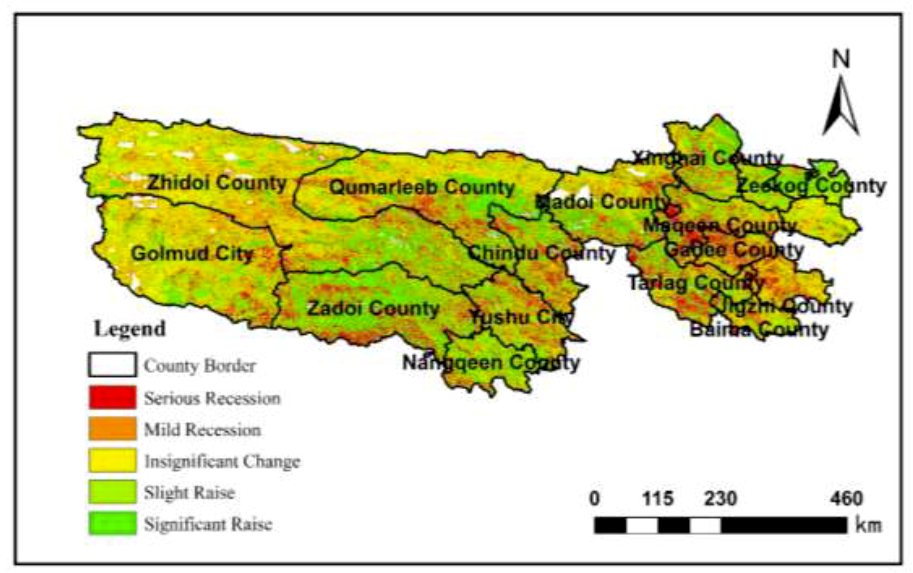
4.1. Overall Characteristics of the TRHR
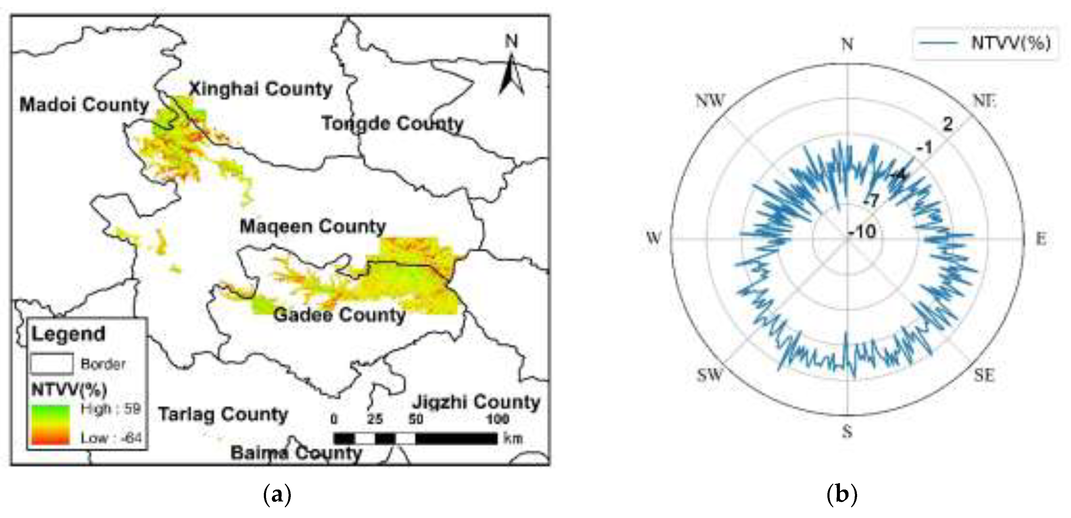
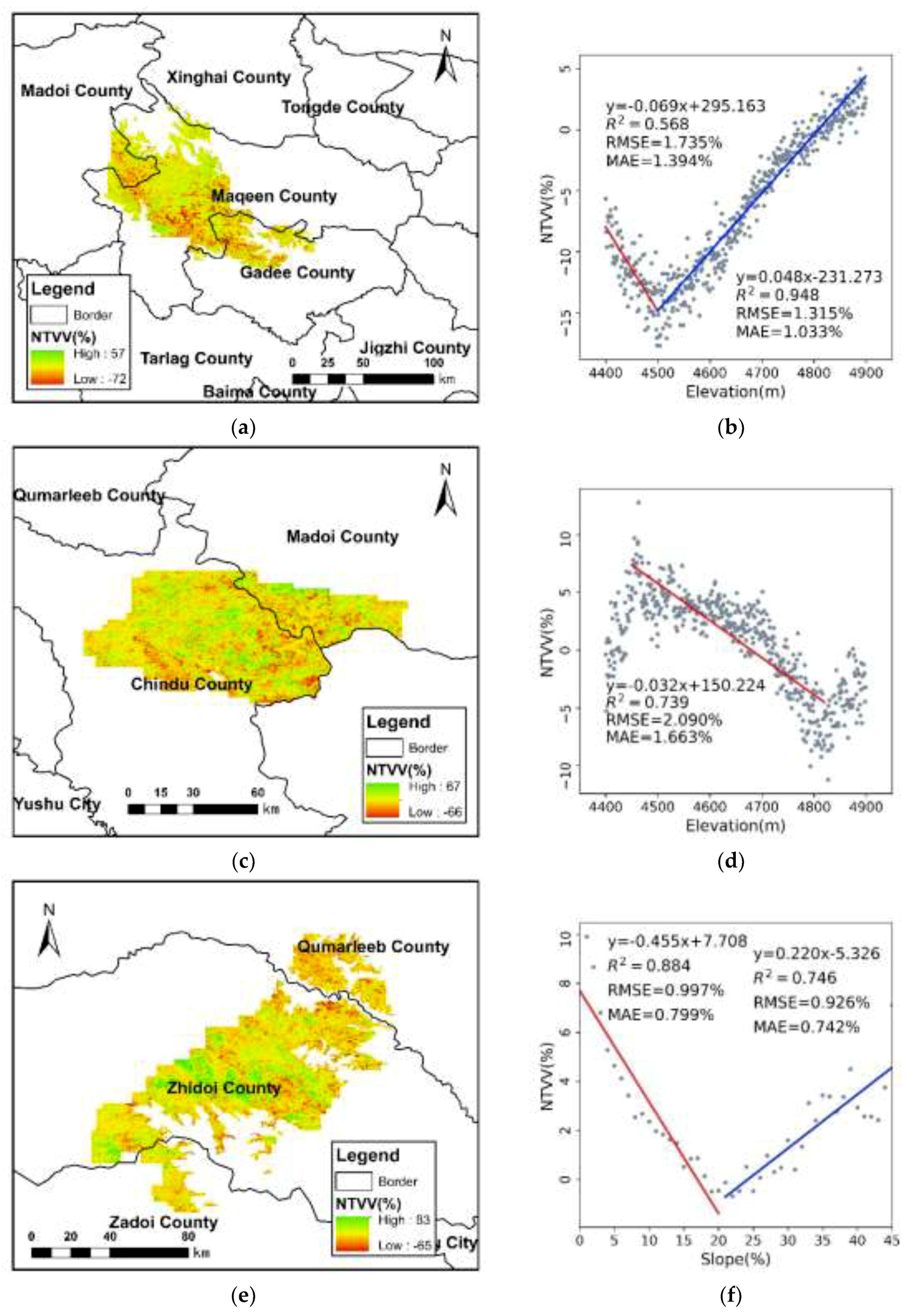
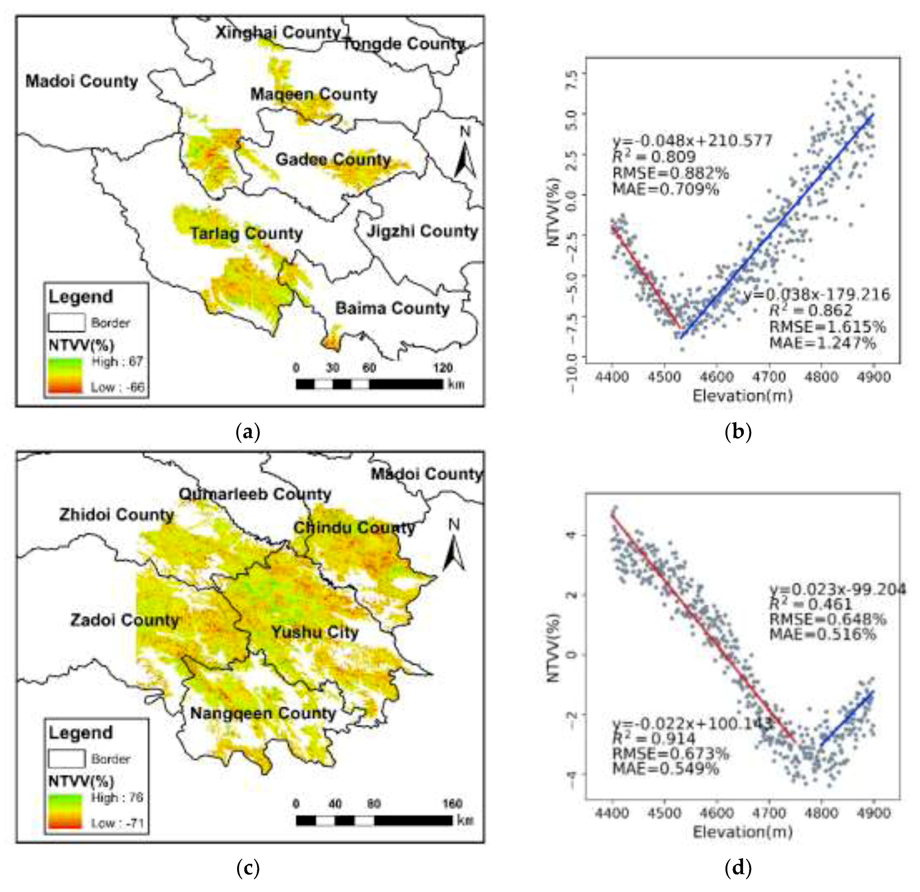
4.2. Area with Significantly NTV Decrease
4.3. Areas with High NTVV Standard Deviation
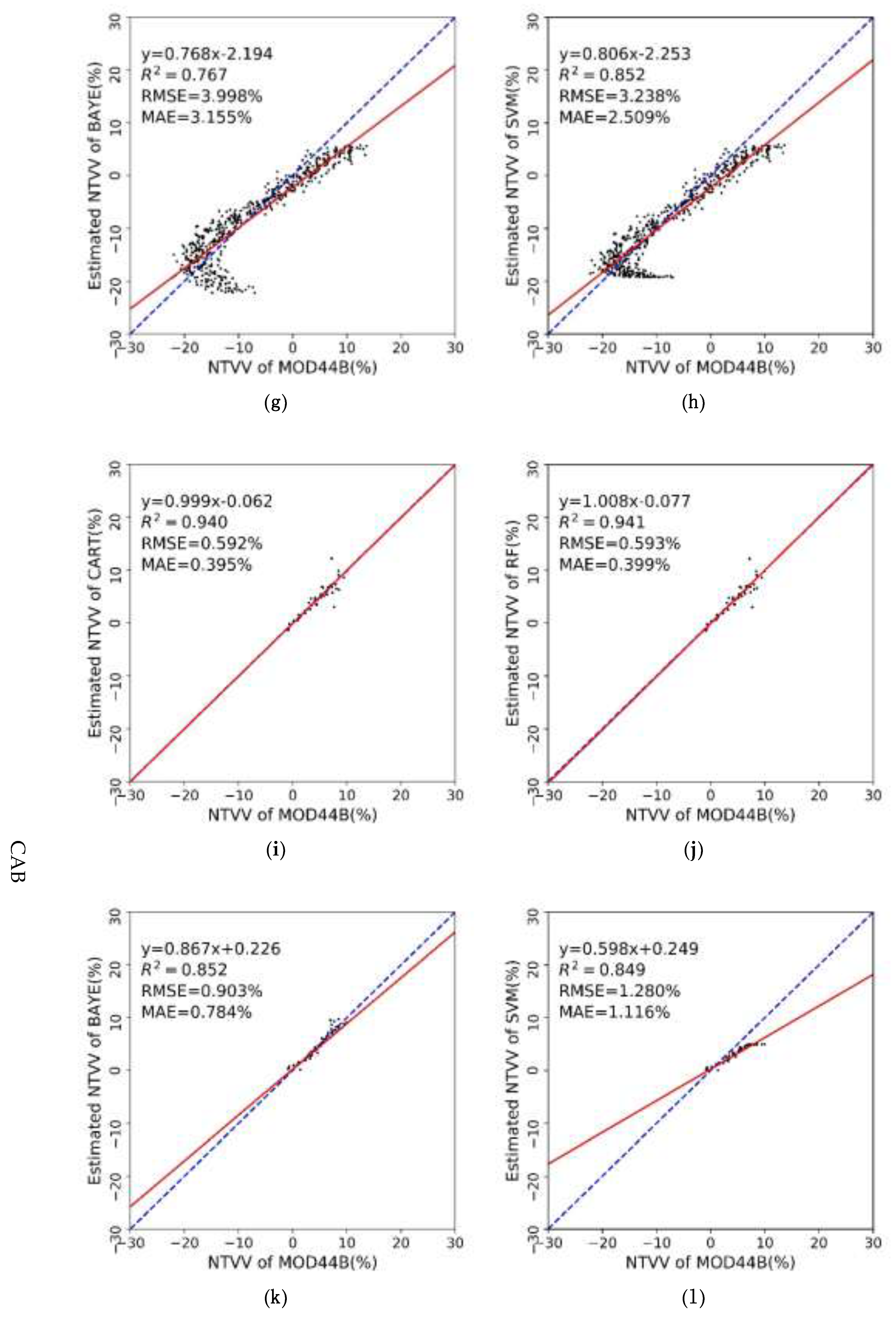
4.4. Machine Learning Results Evaluation
4.5. Evaluation of Machine Learning Results without AD and TA Methods
4.6. Evaluation of Machine Learning Results without TA Method
5. Discussion
6. Conclusions
Author Contributions
Acknowledgments
Conflicts of Interest
References
- Liu, X.F.; Zhang, J.S.; Zhu, X.F.; Pan, Y.Z.; Liu, Y.X.; Zhang, D.H.; Lin, Z.H. Spatiotemporal changes in vegetation cover and its driving factors in the Three-River Headwaters Region during 2000–2011. J. Geogr. Sci. 2014, 24, 288–302. [Google Scholar] [CrossRef]
- Shen, X.J.; An, R.; Feng, L.; Ye, N.; Zhu, L.; Li, M. Vegetation changes in the Three-River Headwaters Region of the Tibetan Plateau of China. Ecol. Indic. 2018, 93, 804–812. [Google Scholar] [CrossRef]
- Sun, Q.L.; Li, B.L.; Xu, L.L.; Zhang, T.; Ge, J.S.; Li, F. Analysis of NDVI change trend and its impact factors in the Three-River Headwater Region from 2000 to 2013. J. Geo-Inf. Sci. 2016, 18, 1707–1716. [Google Scholar]
- Liu, J.Y.; Xu, X.L.; Shao, Q.Q. The spatial and temporal characteristics of grassland degradation in the Three-river Headwaters Region in Qinghai Province. Acta Geogr. Sin. 2008, 63, 364–376. [Google Scholar]
- Shao, Q.Q.; Cao, W.; Fan, J.W.; Huang, L.; Xu, X.L. Effects of an ecological conservation and restoration project in the Three-River Source Region. China. J. Geogr. Sci. 2017, 27, 183–204. [Google Scholar] [CrossRef]
- Liu, L.L.; Cao, W.; Shao, Q.Q. Characteristics of Land Use/Cover and Macroscopic Ecological Changes in the Headwaters of the Yangtze River and of the Yellow River over the Past 30 Years. Sustainability 2016, 8, 237. [Google Scholar] [CrossRef]
- Zhou, W.; Yang, H.; Huang, L.; Chen, C.; Lin, X.; Hu, Z. Grassland degradation remote sensing monitoring and driving factors quantitative assessment in China from 1982 to 2010. Ecol. Indic. 2017, 83, 303–313. [Google Scholar] [CrossRef]
- Asrar, G.; Weiser, R.L.; Johnson, D.E.; Kanemasu, E.T.; Kileen, J.M. Distinguishing among tallgrass prairie cover types from measurements of multispectral reflectance. Remote Sens. Environ. 1986, 19, 159–169. [Google Scholar] [CrossRef]
- Alfredo, C.D.; Emilio, C.W.; Ana, C. Satellite remote sensing analysis to monitor desertification processes in the crop-rangeland boundary of Argentina. J. Arid Environ. 2002, 52, 121–133. [Google Scholar]
- Lu, D.; Batistella, M.; Mausel, P.; Moran, E. Mapping and monitoring land degradation risks in the Western Brazilian Amazon using multitemporal Landsat TM/ETM+ images. Land Degrad. Dev. 2007, 18, 41–54. [Google Scholar] [CrossRef]
- Schmidt, S.; Alewell, C.; Meusburger, K. Mapping spatio-temporal dynamics of the cover and management factor (C-factor) for grasslands in Switzerland. Remote Sens. Environ. 2018, 211, 89–104. [Google Scholar] [CrossRef]
- Wang, X.H.; Wang, B.T.; Xu, X.Y.; Liu, T.; Duan, Y.J.; Zhao, Y. Spatial and temporal variations in surface soil moisture and vegetation cover in the Loess Plateau from 2000 to 2015. Ecol. Indic. 2018, 95, 320–330. [Google Scholar] [CrossRef]
- Liu, Y.; Li, L.H.; Chen, X.; Zhang, R.; Yang, J.M. Temporal-spatial variations and influencing factors of vegetation cover in Xinjiang from 1982 to 2013 based on GIMMS-NDVI3g. Glob. Planet. Chang. 2018, 169, 145–155. [Google Scholar] [CrossRef]
- Li, Z.; Huffman, T.; McConkey, B.; Townley-Smith, L. Monitoring and modeling spatial and temporal patterns of grassland dynamics using time-series MODIS NDVI with climate and stocking data. Remote Sens. Environ. 2013, 138, 232–244. [Google Scholar] [CrossRef]
- Li, J.Y.; Yang, X.C.; Jin, Y.X.; Yang, Z.; Huang, W.G.; Zhao, L.N.; Gao, T.; Yu, H.D.; Ma, H.L.; Qin, Z.H.; et al. Monitoring and analysis of grassland desertification dynamics using Landsat images in Ningxia, China. Remote Sens. Environ. 2013, 138, 19–26. [Google Scholar] [CrossRef]
- Si, Y.L.; Schlerf, M.; Zurita-Milla, R.; Skidmore, A.; Wang, T.J. Mapping spatio-temporal variation of grassland quantity and quality using MERIS data and the PROSAIL model. Remote Sens. Environ. 2012, 121, 415–425. [Google Scholar] [CrossRef]
- Fu, B.J.; Liu, G.H.; Lv, Y.H.; Chen, L.D.; Ma, K.M. Ecoregions and ecosystem management in China. Int. J. Sustain. Dev. World Ecol. 2004, 11, 397–409. [Google Scholar] [CrossRef]
- Chen, B.X.; Zhang, X.Z.; Tao, J.; Wu, J.; Wang, J.; Shi, P. The impact of climate change and anthropogenic activities on alpine grassland over the Qinghai-Tibet Plateau. Agric. Forest Meteorol. 2014, 189–190, 11–18. [Google Scholar] [CrossRef]
- Wang, B.; Tao, Q.; Hoskins, B.; Wu, G.; Liu, Y. Tibetan Plateau warming and precipitation changes in East Asia. Geophys. Res. Lett. 2008, 35, L14702. [Google Scholar] [CrossRef]
- The People’s Government of Qinghai Province. The Second Stage Planning on Ecological Protection and Construction in Qinghai Sanjiangyuan Nature Reserve; The People’s Government of Qinghai Province: Xining, China, 2013.
- Niu, T.L.; Liu, X.H.; Li, Z.Y.; Gao, Y.Y.; De, K.J.; Wang, X.; Shi, H.L. The spatio-temporal changes of the grassland in Madoi County, the source region of the Yellow River during 1990–2009. Environ. Sci. Technol. 2013, 36, 438–442. [Google Scholar]
- Zhou, W.; Gang, C.C.; Li, J.L.; Zhang, C.B.; Mu, S.J.; Sun, Z.G. Spatial-temporal dynamics of grassland cover and its response to climate change in China during 1982–2010. Acta Geogr. Sin. 2014, 69, 15–30. [Google Scholar]
- Ma, T.X.; Song, X.F.; Zhao, X.; Li, R.H. Spatiotemporal Variation of Vegetation Cover and Its Affecting Factors in the Headwaters of the Yellow River during the Period of 2000-2010. Arid Zone Res. 2016, 33, 1217–1225. [Google Scholar]
- Xiao, T.; Wang, C.Z.; Feng, M.; Qu, R.; Zhai, J. Dynamic Characteristic of vegetation cover in the Three-River Source Region from 2000 to 2011. Acta Agrestia Sin. 2014, 22, 39–45. [Google Scholar]
- Fan, J.W.; Shao, Q.Q.; Liu, J.Y.; Wang, J.B.; Harris, W.; Chen, Z.Q. Assessment of effects of climate change and grazing activity on grassland yield in the Three Rivers Headwaters Region of Qinghai–Tibet Plateau, China. Environ. Monit. Assess. 2010, 170, 571–584. [Google Scholar] [CrossRef] [PubMed]
- Wang, J.; Zhao, Y.Y.; Li, C.C.; Yu, L.; Liu, D.; Gong, P. Mapping global land cover in 2001 and 2010 with spatial-temporal consistency at 250 m resolution. ISPRS J. Photogramm. Remote Sens. 2015, 103, 38–47. [Google Scholar] [CrossRef]
- Sangermano, F.; Bol, L.; Galvis, P.; Gullison, R.E; Hardner, J.; Ross, G.S. Forest baseline and deforestation map of the Dominican Republic through the analysis of time series of MODIS data. Data Brief 2015, 4, 363–367. [Google Scholar] [CrossRef] [PubMed]
- Gessner, U.; Machwitz, M.; Conrad, C.; Dech, S. Estimating the Fractional Cover of Growth Forms and Bare Surface in Savannas. A Multi-resolution Approach based on Regression Tree Ensembles. Remote Sens. Environ. 2013, 129, 90–102. [Google Scholar] [CrossRef]
- Price, D.T.; McKenney, D.W.; Nalder, I.A.; Hutchinson, M.F.; Kesteven, J.L. A comparison of two statistical methods for spatial interpolation of Canadian monthly mean climate data. Agric. Forest Meteorol. 2000, 101, 81–94. [Google Scholar] [CrossRef]
- McKenney, D.W.; Pedlar, J.H.; Papadopol, P.; Hutchinson, M.F. The development of 1901–2000 historical monthly climate models for Canada and the United States. Agric. Forest Meteorol. 2006, 138, 69–81. [Google Scholar] [CrossRef]
- Jarvis, A.; Reuter, H.I.; Nelson, A.; Guevara, E. Hole-Filled SRTM for the Globe Version 4. 2008. Available online: http://srtm.csi.cgiar.org (accessed on 1 October 2018).
- Tabulate Area. Available online: http://pro.arcgis.com/en/pro-app/tool-reference/spatial-analyst/tabulate-area.htm (accessed on 9 August 2018).
- Burrows, W.R.; Benjamin, M.; Beauchamp, S.; Lord, E.R.; McCollor, D.; Thomson, B. CART decision-tree statistical analysis and prediction of summer season maximum surface ozone for the Vancouver, Montreal, and Atlantic regions of Canada. J. Appl. Meteorol. 1995, 34, 1848–1862. [Google Scholar] [CrossRef]
- Westreich, D.; Lessler, J.; Funk, M.J. Propensity score estimation: Neural networks, support vector machines, decision trees (CART), and meta-classifiers as alternatives to logistic regression. J. Clin. Epidemiol. 2010, 63, 826–833. [Google Scholar] [CrossRef] [PubMed]
- Breiman, L. Random forests. Mach. Learn. 2001, 45, 5–32. [Google Scholar] [CrossRef]
- Pal, M. Random forest classifier for remote sensing classification. Int. J. Remote Sens. 2005, 26, 217–222. [Google Scholar] [CrossRef]
- Pedregosa, F.; Varoquaux, G.; Gramfort, A.; Michel, V.; Thirion, B.; Grisel, O.; Blondel, M.; Prettenhofer, P.; Weiss, R.; Dubourg, V.; et al. Scikit-learn: Machine learning in Python. J. Mach. Learn. Res. 2011, 12, 2825–2830. [Google Scholar]
- Tipping, M.E. Sparse Bayesian Learning and the Relevance Vector Machine. J. Mach. Learn. Res. 2001, 1, 211–244. [Google Scholar]
- Vapnik, V.; Vashist, A. A new learning paradigm: Learning using privileged information. Neural Netw. 2009, 22, 544–557. [Google Scholar] [CrossRef] [PubMed]
- Shao, Q.Q.; Fan, J.W.; Liu, J.Y.; Huang, L.; Cao, W.; Liu, L.L. Target-based Assessment on Effects of First-stage Ecological Conservation and Restoration Project in Three-river Source Region, China and Policy Recommendations. Bull. Chin. Acad. Sci. 2017, 32, 35–44. [Google Scholar]
- Li, S.S.; Zhang, M.J.; Wang, B.L.; Li, X.F.; Luo, S.F. Spatial difference of precipitation variation in Three-river headwaters region of China in recent 51 years. Chin. J. Ecol. 2012, 31, 2635–2643. [Google Scholar]
- Yi, X.S.; Yin, Y.Y.; Li, G.S.; Peng, J.T. Temperature Variation in Recent 50 Years in the Three-River Headwaters Region of Qinghai Province. Sci. Geogr. Sin. 2011, 66, 1451–1465. [Google Scholar]
- Shao, J.A.; Lu, Q.S.; Zhang, X.Y. Remote Sensing-based Characteristics of Grassland Degradation in the Arid Western Three-River Sources Regions of Qinghai in the Past 30 Years. J. Nat. Resour. 2008, 23, 643–656. [Google Scholar]
- Chen, H. Response of Vegetation Community Characteristic and Soil Physico-Chemical Properties Grazing Intensity on Kobresia Pygmaea Meadow of Qinghai-Tibet Plateau; Northwest A&F University: Yangling, China, 2012. [Google Scholar]
- Wei, H.L.; Qi, Y.J. Analysis of grassland degradation of the Tibet Plateau and human driving forces based on remote sensing. Pratacultural Sci. 2016, 33, 2576–2586. [Google Scholar]
- Gao, Q.Z.; Li, Y.E.; Lin, E.D. Temporal and Spatial Distribution of Grassland Degradation in Northern Tibet. Sci. Geogr. Sin. 2005, 60, 965–973. [Google Scholar]
- Beullens, J.; Van de Velde, D.; Nyssen, J. Impact of slope aspect on hydrological rainfall and on the magnitude of rill erosion in Belgium and northern France. Catena 2014, 114, 129–139. [Google Scholar] [CrossRef]
- Ling, B.; Yu, M. Sensitivity Factors of Slope Gradient and Slope Direction of Landslides in Daguan County, Yunnan. Urban Geol. 2015, 10, 66–68. [Google Scholar]
- Wang, Y.F.; Li, M.S.; Lu, Y.D.; Luo, C.Y. Analysis of definition of slope gradient criterion for farmland to forest. Sci. Tech. Inf. Soil Water Conserv. 2004, 6, 25–27. [Google Scholar]
- Zhang, X.; Li, P.; Li, Z.B.; Yu, G.Q.; Li, C. Effects of precipitation and different distributions of grass strips on runoff and sediment in the loess convex hillslope. Catena 2018, 162, 130–140. [Google Scholar] [CrossRef]
- Feng, Y.Q.; Liang, S.H.; Wu, Q.B.; Chen, J.W.; Tian, X.; Wu, P. Vegetation responses to permafrost degradation in the Qinghai-Tibetan Plateau. J. Beijing Normal Univ. (Nat. Sci.) 2016, 52, 311–316. [Google Scholar]
- Yue, G.Y.; Zhao, L.; Zhao, Y.H.; Du, E.J.; Wang, Q.; Wang, Z.W.; Qiao, Y.P. Relationship between soil properties in permafrost active layer and surface vegetation in Xidatan on the Qinghai-Tibetan Plateau. J. Glaciol. Geocryol. 2013, 35, 565–573. [Google Scholar]
- Wang, X.Y.; Yi, S.H.; Wu, Q.B. The role of permafrost and soil water in distribution of alpine grassland and its NDVI dynamics on the Qinghai-Tibetan Plateau. Glob. Planet. Chang. 2016, 147, 40–53. [Google Scholar] [CrossRef]
- Sun, F.D.; Long, R.J.; Guo, Z.G.; Liu, W.; Gan, Y.M.; Chen, W.Y. Effects of rodents activities on plant community and soil environment in alpine meadow. Pratacultural Sci. 2011, 28, 146–151. [Google Scholar]
- Zhu, L.; Dong, S.K.; Wen, L. Effect of Cultivated Pasture on Recovering Soil Nutrient of “Blackbeach” in the Alpine Region of Headwater Areas of Qinghai-Tibetan Plateau, China. Procedia Environ. Sci. 2010, 2, 1355–1360. [Google Scholar] [CrossRef]
- Zhou, H.K.; Zhou, L.; Zhao, X.Q.; Liu, W.; Yan, Z.L.; Shi, Y. Degradation process and integrated treatment of “black soil beach” grassland in the source regions of Yangtze and Yellow Rivers. Chin. J. Ecol. 2003, 22, 51–55. [Google Scholar]
- Peng, J.; Pan, Y.J.; Liu, Y.X.; Zhao, H.; Wang, Y. Linking ecological degradation risk to identify ecological security patterns in a rapidly urbanizing landscape. Habitat Int. 2018, 71, 110–124. [Google Scholar] [CrossRef]
- Peng, J.; Yang, Y.; Liu, Y.X.; Hu, Y.; Du, Y.; Meersmans, J. Linking ecosystem services and circuit theory to identify ecological security patterns. Sci. Total Environ. 2018, 644, 781–790. [Google Scholar] [CrossRef] [PubMed]
- Zhang, L.P.; Peng, J.; Liu, Y.X.; Wu, J. Coupling ecosystem services supply and human ecological demand to identify landscape ecological security pattern: A case study in Beijing-Tianjin-Hebei region, China. Urban Ecosyst. 2017, 20, 701–714. [Google Scholar] [CrossRef]
- Feng, S.R.; Guo, L.; Li, D.D.; Huang, Q. Spatial patterns of landscape change in the Three Rivers Headwaters Region of China, 1987–2015. Acta Ecol. Sin. 2018, 38, 76–80. [Google Scholar] [CrossRef]
- Zheng, Y.T.; Han, J.C.; Fassnacht, S.R.; Xie, S.; Lv, E. Vegetation response to climate conditions based on NDVI simulations using stepwise cluster analysis for the Three-River Headwaters region of China. Ecol. Indic. 2017, 92, 18–29. [Google Scholar] [CrossRef]


| Class | DEM (m) | TEM (°C) | PRE (mm) |
|---|---|---|---|
| A | <4400 | <−3.31 | <476.88 |
| B | ≥4400 & <4900 | ≥−3.31 | ≥476.88 |
| C | ≥4900 |
| Study Areas * | Code Combination Definitions | ||
|---|---|---|---|
| 1st Letter: DEM (m) | 2nd Letter: TEM (°C) | 3rd Letter: PRE (mm) | |
| AAA | <4400 | <−3.31 | <476.88 |
| AAB | <4400 | <−3.31 | ≥476.88 |
| ABA | <4400 | ≥−3.31 | <476.88 |
| ABB | <4400 | ≥−3.31 | ≥476.88 |
| BAA | ≥4400 & <4900 | <−3.31 | <476.88 |
| BAB | ≥4400 & <4900 | <−3.31 | ≥476.88 |
| BBA | ≥4400 & <4900 | ≥−3.31 | <476.88 |
| BBB | ≥4400 & <4900 | ≥−3.31 | ≥476.88 |
| CAA | ≥4900 | <−3.31 | <476.88 |
| CAB | ≥4900 | <−3.31 | ≥476.88 |
| CBA | ≥4900 | ≥−3.31 | <476.88 |
| CBB | ≥4900 | ≥−3.31 | ≥476.88 |
| Study Areas | Area (km2) | NTVV (%) | Standard Deviation (%) |
|---|---|---|---|
| AAA | 7712 | −0.96 | 8.86 |
| AAB | 4944 | −1.98 | 13.63 |
| ABA | 19,551 | 2.34 | 10.71 |
| ABB | 54,386 | 2.54 | 11.34 |
| BAA | 70,579 | 0.82 | 9.24 |
| BAB | 25,855 | 0.78 | 14.61 |
| BBA | 34,092 | 0.66 | 9.7 |
| BBB | 47,224 | 1.18 | 14.98 |
| CAA | 48,276 | −0.15 | 5.19 |
| CAB | 12,577 | −0.33 | 10.98 |
| CBA | 1016 | 1.31 | 7.91 |
| CBB | 8930 | −0.74 | 13.36 |
| Study Areas | ML Method | R2 | RMSE (%) | MAE (%) |
|---|---|---|---|---|
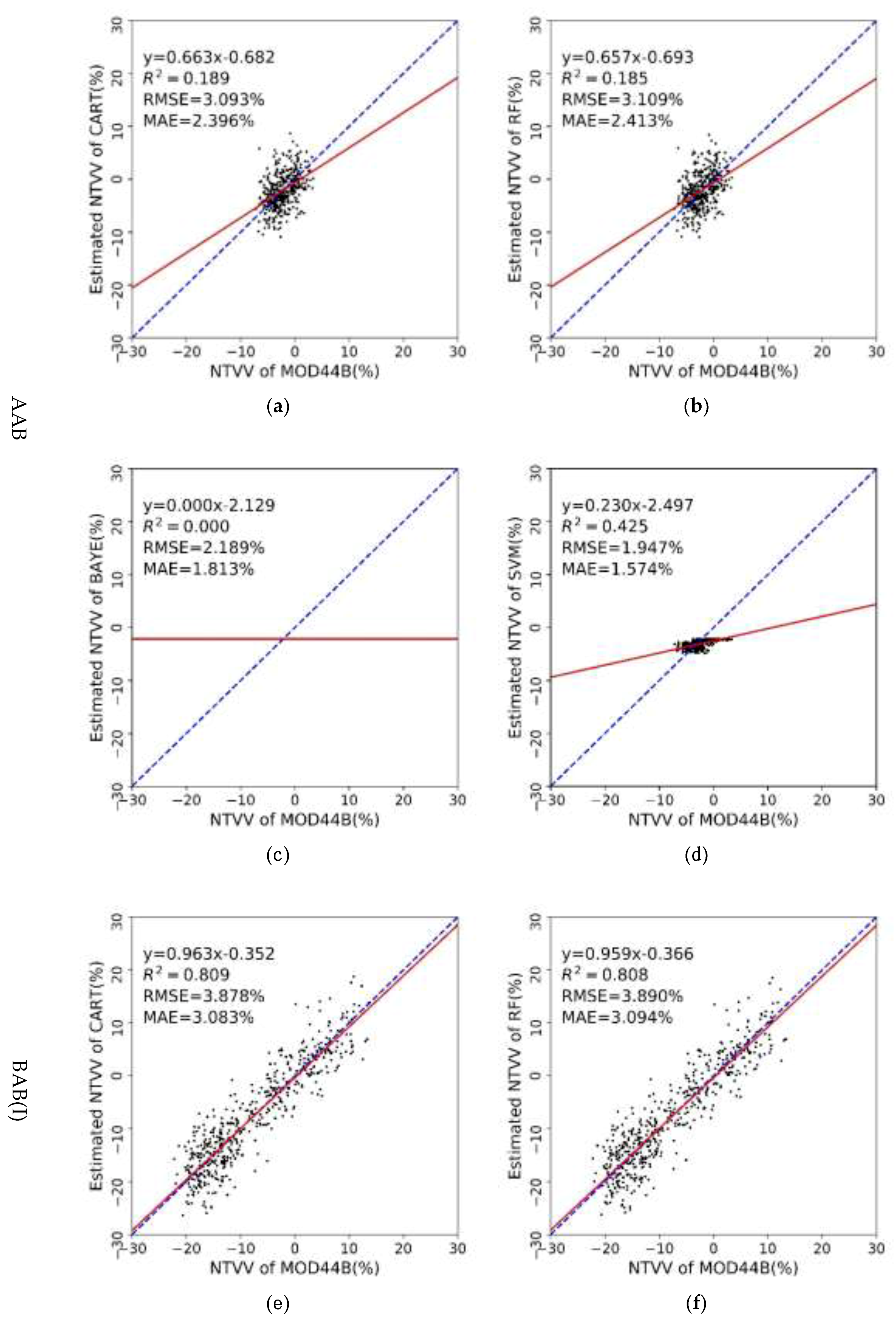
| AAB | CART | 0.189 | 3.093 | 2.396 |
| RF | 0.185 | 3.109 | 2.413 | |
| BAYE | 0.000 | 2.189 | 1.813 | |
| SVM | 0.425 | 1.947 | 1.574 | |
| BAB(I) | CART | 0.809 | 3.878 | 3.083 |
| RF | 0.808 | 3.890 | 3.094 | |
| BAYE | 0.767 | 3.998 | 3.155 | |
| SVM | 0.852 | 3.238 | 2.509 | |
| BAB(II) | CART | 0.576 | 4.350 | 3.386 |
| RF | 0.578 | 4.337 | 3.388 | |
| BAYE | 0.721 | 2.976 | 2.276 | |
| SVM | 0.781 | 4.672 | 4.128 | |
| BAB(III) | CART | 0.940 | 0.949 | 0.595 |
| RF | 0.942 | 0.928 | 0.598 | |
| BAYE | 0.569 | 2.394 | 1.909 | |
| SVM | 0.830 | 4.317 | 3.580 | |
| BBB(I) | CART | 0.481 | 4.066 | 3.162 |
| RF | 0.482 | 4.034 | 3.148 | |
| BAYE | 0.032 | 4.368 | 3.409 | |
| SVM | 0.785 | 2.504 | 2.076 | |
| BBB(II) | CART | 0.728 | 1.846 | 1.462 |
| RF | 0.727 | 1.856 | 1.465 | |
| BAYE | 0.749 | 1.631 | 1.240 | |
| SVM | 0.885 | 2.597 | 2.197 | |
| BBB(III) | CART | 0.225 | 0.951 | 0.448 |
| RF | 0.230 | 0.949 | 0.440 | |
| BAYE | 0.302 | 0.692 | 0.458 | |
| SVM | 0.070 | 2.469 | 2.366 | |
| CAB | CART | 0.940 | 0.592 | 0.395 |
| RF | 0.941 | 0.593 | 0.399 | |
| BAYE | 0.852 | 0.903 | 0.784 | |
| SVM | 0.849 | 1.280 | 1.116 | |
| CBB | CART | 0.947 | 0.815 | 0.618 |
| RF | 0.949 | 0.796 | 0.594 | |
| BAYE | 0.949 | 0.821 | 0.707 | |
| SVM | 0.969 | 1.347 | 1.161 |
| Study Areas | W/WO TA Method | R2 | RMSE (%) | MAE (%) |
|---|---|---|---|---|
| AAB | W | 0.185 | 3.109 | 2.413 |
| WO | 0.011 | 24.018 | 17.527 | |
| BAB(I) | W | 0.808 | 3.890 | 3.094 |
| WO | 0.075 | 23.858 | 18.076 | |
| BAB(II) | W | 0.578 | 4.337 | 3.388 |
| WO | 0.015 | 29.650 | 22.676 | |
| BAB(III) | W | 0.942 | 0.928 | 0.598 |
| WO | 0.013 | 27.222 | 20.774 | |
| BBB(I) | W | 0.482 | 4.034 | 3.148 |
| WO | 0.018 | 26.235 | 20.001 | |
| BBB(II) | W | 0.727 | 1.856 | 1.465 |
| WO | 0.008 | 25.233 | 19.003 | |
| BBB(III) | W | 0.230 | 0.949 | 0.440 |
| WO | 0.000 | 30.145 | 22.545 | |
| CAB | W | 0.941 | 0.593 | 0.399 |
| WO | 0.008 | 23.092 | 17.323 | |
| CBB | W | 0.949 | 0.796 | 0.594 |
| WO | 0.036 | 24.847 | 19.044 |
© 2018 by the authors. Licensee MDPI, Basel, Switzerland. This article is an open access article distributed under the terms and conditions of the Creative Commons Attribution (CC BY) license (http://creativecommons.org/licenses/by/4.0/).
Share and Cite
Liu, N.; Yang, Y.; Yao, L.; Yue, X. A Regionalized Study on the Spatial-Temporal Changes of Grassland Cover in the Three-River Headwaters Region from 2000 to 2016. Sustainability 2018, 10, 3539. https://doi.org/10.3390/su10103539
Liu N, Yang Y, Yao L, Yue X. A Regionalized Study on the Spatial-Temporal Changes of Grassland Cover in the Three-River Headwaters Region from 2000 to 2016. Sustainability. 2018; 10(10):3539. https://doi.org/10.3390/su10103539
Chicago/Turabian StyleLiu, Naijing, Yaping Yang, Ling Yao, and Xiafang Yue. 2018. "A Regionalized Study on the Spatial-Temporal Changes of Grassland Cover in the Three-River Headwaters Region from 2000 to 2016" Sustainability 10, no. 10: 3539. https://doi.org/10.3390/su10103539
APA StyleLiu, N., Yang, Y., Yao, L., & Yue, X. (2018). A Regionalized Study on the Spatial-Temporal Changes of Grassland Cover in the Three-River Headwaters Region from 2000 to 2016. Sustainability, 10(10), 3539. https://doi.org/10.3390/su10103539