Multi-Depot Vehicle Routing Optimization Considering Energy Consumption for Hazardous Materials Transportation

Abstract

Focusing on the multi-depot vehicle routing problem (MDVRP) for hazardous materials transportation, this paper presents a multi-objective optimization model to minimize total transportation energy consumption and transportation risk. A two-stage method (TSM) and hybrid multi-objective genetic algorithm (HMOGA) are then developed to solve the model. The TSM is used to find the set of customer points served by each depot through the global search clustering method considering transportation energy consumption, transportation risk, and depot capacity in the first stage, and to determine the service order of customer points to each depot by using a multi-objective genetic algorithm with the banker method to seek dominant individuals and gather distance to keep evolving the population distribution in the second stage, while with the HMOGA, customer points serviced by the depot and the serviced orders are optimized simultaneously. Finally, by experimenting on two cases with three depots and 20 customer points, the results show that both methods can obtain a Pareto solution set, and the hybrid multi-objective genetic algorithm is able to find better vehicle routes in the whole transportation network. Compared with distance as the optimization objective, when energy consumption is the optimization objective, although distance is slightly increased, the number of vehicles and energy consumption are effectively reduced.

1. Introduction

Hazardous materials can be toxic, corrosive, inflammable, and explosive, but also are necessary for the development of industry and agriculture. How to choose one or more transportation routes for hazardous materials with low energy consumption and low risk has become a very important topic with practical significance to ensure personal, property, and environmental security as well as economic sustainability.

According to statistics, the daily amount of hazardous materials being transported in China exceeds 1 million tons, and the total amount per year exceeds 400 million tons [1]. These large quantities of hazardous materials form a dangerous flowing source on the roads. If an accident occurs, it could cause damage to nearby people and the surrounding environment. Alp et al. [2] studied the effects of meteorologic conditions and wind direction probabilities on the consequences of accidents, and proposed a three-integral mathematical evaluation model for calculating individual and social risks. Leonelli et al. [3] proposed a new personal and social risk assessment model, introducing risk factors such as transportation mode, hazardous materials category, meteorologic conditions, wind direction probability, and seasonal attributes, and considered the impact of population distribution, which greatly improved the accuracy of risk assessment for hazardous materials transportation. Based on a statistical analysis of accidents, Fabiano et al. [4] discussed risk factors from the aspects of road characteristics, weather conditions, and traffic conditions, and proposed a risk assessment model for the hazardous materials transportation process at accident sites. Based on the route segment–specific (location-specific) accident rate, Chakrabarti et al. [5] estimated route segment total risk to measure the average number of persons likely to be exposed to all possible consequence scenarios by computing and comparing the loss of containment and spillage probabilities for different route segments. Taking the length and quality of roads, the population density in different segments of the roads, types of hazardous materials, and types of vehicles into consideration, Faghih-Roohi et al. [6] proposed a dynamic value-at-risk model. Mohammadi et al. [7] designed a reliable hazardous materials transportation network based on four factors: distance from the incident source, number of people exposed to the risk, number of hazardous materials shipments passing that segment, and the characteristics of the road type. With the rapid development of Geographic Information System (GIS) technology, it has also been applied to risk assessment for hazardous materials transportation (Bubbico et al. [8], Sahnoon et al. [9], Chen et al. [10]). Visual map display and data analysis functions provide convenience and improve accuracy for risk assessment during the transportation of hazardous materials. It can be seen that scholars have made many contributions to the problem of transporting hazardous materials. The risk of transporting hazardous materials is related to many uncertain factors, and it is difficult to measure accurately, but it is still a factor that must be considered.

In addition to risk, energy consumption is also an important factor to consider in reducing the transportation costs of enterprises, reducing carbon emissions, and achieving sustainable development of hazardous materials transportation. There are many factors that affect transportation energy consumption, but they can be roughly classified into categories such as vehicle construction, transportation environment, and driver strategies. Factors influencing fuel consumption have been studied by Bigazzi et al. [11], Demir et al. [12], and Suzuki [13]. Trucks have to overcome various obstacles while transporting hazardous materials, such as speed, road gradient, and payload. These are key factors that affect energy consumption. Bektaş and Laporte [14] analyzed the relationship between vehicle load, speed, and total cost, and proposed that minimizing the cumulative load alone does not necessarily lead to energy minimization, particularly when there are time window restrictions. Demir et al. [15] derived an optimum driving speed and showed that reductions in emissions could be achieved by varying speed over a network. It should be noted that the optimum driving speed varies to a certain degree between geographic areas due to speed limits and traffic density. Given the fact that the shortest distance may not be the optimal solution for the purpose of lowering fuel consumption, Xiao et al. [16] developed route schedules with lower fuel costs by better managing the trade-off between the total distance and the priority of serving customers with larger demands. Suzuki [17] indicated that significant savings in fuel consumption may be realized by delivering heavy items in the early segments of a tour and lighter items in the later segments. In fact, transportation costs are more related to energy consumption than distance. Therefore, for hazardous materials transportation, considering the factors that affect energy consumption, it is more practical to find one or more low-energy vehicle routes as the optimization objective.

The transportation route is a key factor to guarantee that hazardous materials are transported safely and economically, which many experts and scholars have been studying. Batta et al. classified transportation risk into road risk and node risk [18]. Karkazis et al. [19] formulated the routing problem of transporting hazardous materials as an optimization problem, with the objective of minimizing transportation risk and costs. Meng et al. [20] used the dynamic programming method to solve the transportation route optimization problem. Liu et al. [21] applied a multilevel fuzzy comprehensive evaluation method to optimizing hazardous materials transportation routing. Das et al. [22] explored the routing problem in a transportation network with the capacity limit, and developed a multi-objective algorithm to find nondominated solutions. Pradhananga et al. [23] chose minimum transportation time and risk as the optimization objective to search for Pareto optimal solutions. Given the unscientific nature of simply evaluating the total risk of a fleet as a whole without considering individual vehicle risk, Wang et al. [24] developed a two-stage exact algorithm based on the ε-constraint method to solve the proposed problem. Alrukaibi et al. [25] designed a risk/cost algorithm using available data from Kuwait. For their study, incident probability, incident consequence, and risk assessment were used as the algorithm’s main criteria to identify available alternative routes. Mohammadi et al. [7] proposed a mathematical model for designing a reliable hazardous materials transportation network on the basis of hub location topology under uncertainties; to cope with the uncertainties, they provided a solution framework based on an integration of the chance-constrained programming approach. Obviously, these studies on the routing problem of hazardous materials transportation have been relatively sufficient, and have gone through a study process from a single objective to multi-objective optimization and from certain to uncertain environments. However, energy consumption is not considered in the model, and to solve the model, most studies turned the multi-objective model into a single objective, and finally got an optimal solution instead of the Pareto optimal solution set.

All of the above studies on the vehicle routing problem (VRP) for hazardous materials transportation assumed that there was only one depot. However, there may, in fact, be more than one vehicle depot in a city, and it is of more practical significance to study the VRP with multiple depots for hazardous materials transportation. At present, only a few studies have focused on the multi-depot vehicle routing problem (MDVRP) for hazardous materials transportation. Zhao et al. [26] considered the return trips between collection centers and recycling centers, and developed a multi-objective model with minimization of cost and risk. This optimization problem with two objectives was then transformed into a single objective problem. Du et al. [27] developed a fuzzy bilevel programming model in which the upper-level formulation allocated customers to depots and the lower level determined the optimal routing for each depot. However, the study only considered transportation risk minimization as the optimization objective. In fact, for hazardous materials transportation, in addition to risk, energy consumption is also a major factor that must be considered. This is mainly due to the fact that energy consumption is a key factor in reducing the transportation costs of enterprises, reducing carbon emissions, and achieving sustainable development. To this end, this study aims to find the optimal vehicle routings for the MDVRP considering both transportation risk and energy consumption.

Many heuristic methods have been developed in the context of the VRP, including the tabu search algorithm [28], the genetic algorithm [29], the ant colony algorithm [30], and so on. Compared to the VRP, the MDVRP is more complicated, because it needs to consider which customer point should be serviced by which depot, in addition to considering the vehicle routing for each depot. It is necessary to coordinate the delivery tasks among multiple depots. Gillett and Johnson presented a clustering procedure and a sweep heuristic for each depot [31]. Salhi and Sari proposed a multilevel heuristic method [32]. Giosa et al. [33] summarized and proposed a number of heuristics for the two-stage approach to solving the MDVRP. In order to solve the emergency vehicle routing problem with multiple depots, Qin et al. [34] divided it into two steps, and used the nearest assignment and average distance method to transform the MDVRP into multiple VRPs with a single depot in the first step, and then adopted a genetic algorithm to solve the VRPs with a single depot in the second step. Ho et al. [35] developed two hybrid genetic algorithms. The major difference between the two algorithms is that the initial solutions were generated randomly in the first algorithm, and the initialization procedure was incorporated into the Clarke and Wright savings method and the nearest neighbor heuristic in another algorithm. In summary, the methodologies for MDVRP can be categorized into one-stage and two-stage solving methods.

To sum up, a number of studies have explored the traditional VRP with only one depot. These studies move from single objective optimization to multi-objective optimization and from single solution to a nondominated solution set. However, only a few studies have focused on the MDVRP for hazardous materials transportation, and all of them consider a single objective or do not consider transportation energy consumption, due to the complexity of the problem. Furthermore, these studies rarely consider all depots and customer points to find the optimal Pareto solution set to reduce both transportation risk and energy consumption. The existing research has mainly adopted the two-stage method, which cannot make multiple depots coordinate transportation and dynamically solve the problem. In addition, the existing research only considers one objective or converts multiple objectives into one to solve the problem, and they rarely use multi-objective algorithms to seek an optimal Pareto solution set. Different from the current studies on the MDVRP for hazardous materials transportation, this study aims to obtain the Pareto optimal solution set of noncomparable transportation risk and energy consumption. Finally, a two-stage algorithm (TSM) and a one-stage hybrid multi-objective genetic algorithm (HMOGA) are designed, and the solution optimality between these two algorithms is compared and analyzed.

The rest of this paper is organized as follows: Section 2 describes the MDVRP for hazardous materials transportation, Section 3 establishes an optimization model to minimize transportation risk and energy consumption, Section 4 presents a TSM and HMOGA to solve the proposed model, Section 5 gives numerical examples to analyze the effectiveness of the above two algorithms, and Section 6 gives conclusions.

2. Problem Description

As the name implies, the VRP for hazardous materials transportation with one depot is a problem of vehicle scheduling for a specific depot. All customer points are served by a specific depot. However, in reality, it is very common that multiple depots coordinate the transportation and distribution of hazardous materials. The MDVRP for hazardous materials transportation can be defined as the following:

(1)

There exist several hazardous materials depots, and each depot has enough vehicles to transport the hazardous materials.

(2)

Multiple customer points exist and will be assigned to different depots.

(3)

Each vehicle will service the corresponding customer points and can service several customer points, while each customer point can be serviced only one time by one vehicle.

(4)

After the delivery task is finished, all transportation vehicles will return to their hazardous materials depot.

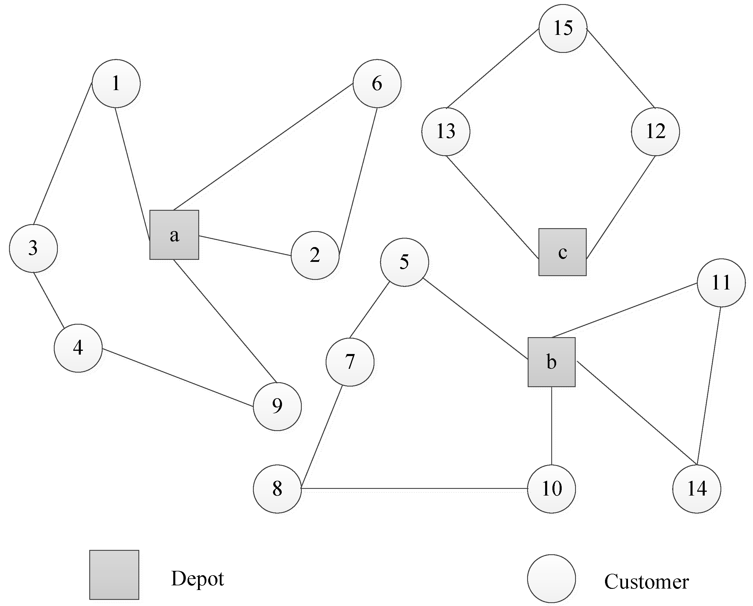
Figure 1 is a sketch of the MDVRP for hazardous materials transportation. It can be seen that with three depots, named a, b, and c, there are 15 customer points, and each customer point can be serviced by only one depot. According to the MDVRP, multiple depots can cooperate with the transportation environment according to customer needs to achieve the global optimal objective.

In the MDVRP, because of the strongly corrosive, highly toxic, explosive, and flammable characteristics of hazardous materials, transportation risk is an optimization objective that must be considered. For enterprises, minimizing transportation costs is paramount. However, low risk means high cost to some extent. Therefore, the MDVRP for hazardous materials transportation should be solved according to the idea of multi-objective optimization, and it is very important to find the Pareto solution set. In many reports in the literature, transportation cost is usually measured by distance and time. However, the shortest transportation distance or time in practice does not mean that transportation cost is the lowest. Compared to distance or time, transportation energy consumption is of great significance to reducing business operating costs, lowering carbon emissions, and achieving sustainable development. Therefore, this paper sets two optimization objectives to minimize risk and energy consumption for hazardous materials transportation.

3. Mathematical Model

3.1. Energy Consumption Evaluation

Rolling resistance, air resistance, and ramp resistance are the main external forces that affect the energy consumption of truck transportation. According to the research in [36], the following formula for calculating power consumption to overcome resistance is used:

$$P_r\left(m,v\right)=c_r·g·m·v$$

(1)

Equation (1) is the power used to overcome rolling resistance during the transportation of hazardous materials, where $P_r\left(m,v\right)$ represents the power consumed by transport equipment with a total weight of m to overcome rolling resistance at speed v (kW); $c_r$ represents the rolling resistance coefficient; g represents gravitational acceleration (m/s²); m represents the total weight of the transport equipment, including the weight of the cargo $m_c$ and the vehicle M(t); and v represents the instantaneous speed of the transport equipment (m/s).

$$P_a\left(v\right)=0.0005c_a·{\rho }_a·z·v^3$$

(2)

Equation (2) is the power consumed to overcome air resistance during transportation, where $P_a\left(v\right)$ is the power consumed to overcome air resistance at speed v (kW); a is the air resistance coefficient; ${\rho }_a$ is air density (kg/m³); and z is the windward area of the vehicle, also known as the front area (m²).

$$P_g\left(m,v,i\right)=m·g·v·i_{ij}$$

(3)

Equation (3) is the power consumed by the truck from node i to node j to overcome ramp resistance during transportation, where $P_g\left(m,v,i\right)$ represents power consumed to overcome ramp resistance at ramp i and transport speed v, and $i_{ij}$ represents the slope of node i to node j.

In addition, the acceleration of trucks while transporting hazardous materials requires a large amount of fuel. According to the literature [37], the energy consumption of trucks accelerating from 0 to $v$ is:

$$W_{num}\left(m,v\right)=\frac{0.504}{7200}m·v^2$$

(4)

The movement of the truck is a real-time change process. Considering that the data are not easy to obtain, this paper uses the average speed $\overline{v}$ and the average slope $\overline{i}$ to calculate the average energy consumption during transportation. Therefore, the average energy consumption of hazardous materials transportation between 2 nodes is:

$${\overline{W}}_{ij}(m,d,\overline{v},\overline{i})=\left(P_r+P_a+P_g\right)·\frac{d_{ij}}{\overline{v}}+n_{num}·d_{ij}·W_{num}$$

(5)

where $d_{ij}$ represents the distance of transportation from node i to node j (km); $\overline{v}$ represents the average speed during transportation (m/s); $\overline{i}$ represents the average slope; and $n_{num}$ represents the average number of accelerations per kilometer (times/km).

3.2. MDVRP Multi-Objective Model for Hazardous Materials Transportation

Hazardous materials transportation risk is usually defined as the product of the accident rate and the potential loss during transportation. The probability of accidents occurring is often affected by time, weather conditions, vehicle type, loading form, and road conditions, and the severity of the consequences are related to the number of people affected, property losses, and weather conditions. In this paper, we use the risk measurement model proposed by Erkut et al. [38] to calculate hazardous materials transportation risk, and regard the number of people affected on both sides of the road as the main indicator for measuring risk:

$$r_{ij}=\frac{2}{1000}{a}_{ij}·p_{ij}·d_{ij}·r_d$$

(6)

where $r_{ij}$ is the risk of road segment (persons), $a_{ij}$ is the accident rate, $p_{ij}$ is the population density (persons/km²), and $r_d$ is the impact radius of the accident (m).

The MDVRP multi-objective model for hazardous materials transportation is:

$$\min Z_1={\displaystyle \sum _{d\in S_0}{\displaystyle \sum _{k\in V_d}{\displaystyle \sum _{i\in S}{\displaystyle \sum _{j\in S_1}{r}_{ij}·x_{ijk}^d}}}}$$

(7)

$$\min Z_2={\displaystyle \sum _{d\in S_0}{\displaystyle \sum _{k\in V_d}{\displaystyle \sum _{i\in S}{\displaystyle \sum _{j\in S}{\overline{W}}_{ij}·x_{ijk}^d}}}}$$

(8)

s.t.

$${\displaystyle \sum _{i\in S}{\displaystyle \sum _{j\in S_{{}_1}}{\displaystyle \sum _{d\in S_0}{x}_{ijk}^d·q_j}\le L_k^d}},\forall k\in V_d$$

(9)

$${\displaystyle \sum _{j\in S_1}{\displaystyle \sum _{k\in V_d}{x}_{ijk}^d}}\le \left|V_d\right|,\forall i\in S_0,\forall d\in S_0$$

(10)

$${\displaystyle \sum _{j\in S_1}{x}_{ijk}^d}-{\displaystyle \sum _{j\in S_1}{x}_{jik}^d}=0,\forall i\in S_0,\forall d\in S_0,\forall k\in V_d$$

(11)

$${\displaystyle \sum _{i\in S}{\displaystyle \sum _{d\in S_0}{\displaystyle \sum _{k\in V_d}{x}_{ijk}^d}=1}},\forall j\in S_1$$

(12)

$${\displaystyle \sum _{j\in S}{\displaystyle \sum _{d\in S_0}{\displaystyle \sum _{k\in V_d}{x}_{ijk}^d}=1}},\forall i\in S_1$$

(13)

$${\displaystyle \sum _{j\in S_0}{x}_{ijk}^d}={\displaystyle \sum _{j\in S_0}{x}_{jik}^d}=0,\forall i\in S_0,\forall d\in S_0,\forall k\in V_d$$

(14)

$$r_{ij}{x}_{ijk}^d\le \mathrm{R},\forall i\in S,\forall j\in S,\forall d\in S_0,\forall k\in V_d$$

(15)

$$x_{ijk}^d=\left\{1,0\right\},\forall i\in S,\forall j\in S,\forall d\in S_0,\forall k\in V_d$$

(16)

In the above model, as the objective functions, Equations (7) and (8), respectively, are used to minimize total transportation risk and energy consumption, and it is worth mentioning that the risk of the delivery vehicle on its return to the depot from the final customer point is not calculated in total risk, while energy is calculated in total transportation energy. In the objective function, $S_0$ is the depot set, here $S_0=\left\{i|i=1,2,\cdots ,m\right\}$; $m$ is the total number of hazardous materials depots; $S_1$ is the customer point set, $S_1=\left\{i|i=1,2,\cdots ,n\right\}$, where $n$ is the number of customer points; $S$ is the transportation network nodes set, here $S=S_0\cup S_1$; $V_d$ is the vehicle set of hazardous materials depot d and $V_d=\left\{k|k=1,2,\cdots ,K\right\}$, $d\in S_0$; and $x_{ijk}^d$ defines the 0–1 integer variable. Equation (9) is the load constraint, which means any vehicle of any depot should satisfy the corresponding load constraint, namely, it cannot overload. In the equation, $q_j$ is the quantity demanded at customer point i and $L_k^d$ is the load capacity of vehicle k from depot d. Equation (10) means the number of vehicles in the depot is limited, and the number of vehicles arranged to transport hazardous materials should not exceed the number owned by the depot. Equation (11) indicates that every vehicle departing from the depot should return to the original depot after finishing the transportation task. Equations (12) and (13) guarantee that each customer point is serviced once and by one vehicle from a depot. Equation (14) means the vehicles cannot depart from one depot and return to another depot. Equation (15) constrains the maximum risk on the segment. Equation (16) denotes that if the route of vehicle $k$ from depot $d$ for transporting hazardous materials contains the road segment from node i to node j, $x_{ijk}^d$ is equal to 1, else $x_{ijk}^d$ equals 0.

4. Solving Methods

Different from single objective optimization, possible conflicts exist between multiple objectives in the multi-objective optimization, and an improved sub-objective might cause the performance of the other one to decrease. Multi-objective optimization generally gets a set of Pareto solutions; elements of the set are called Pareto optimal solutions. In reality, decision-makers select one or more solutions from a Pareto optimal solution set as the optimal solution of a multi-objective optimization problem based on personal preference. For a multi-objective optimization problem, the typical algorithms include niched Pareto genetic algorithm (NPGA) [39], nondominated sorting genetic algorithm-II (NSGA-II) [40], and strong Pareto evolutionary algorithm (SPEA2) [41]. These algorithms have better solution efficiency for particular problems. However, for a specific problem, these algorithms cannot be used directly, but often need to be modified according to the problem properties.

This paper mainly uses genetic algorithm theory to design a method of solving MDVRP for hazardous materials transportation. Based on biological characteristics, the genetic algorithm realizes diversity and global search by operating the population composed of potential solutions. It focuses on the set of individuals, which is consistent with the Pareto solution set of the multi-objective optimization problem. Moreover, the genetic algorithm does not need many mathematical prerequisites, but can deal with all types of objective functions and constraints, and has good performance for combinatorial optimization.

4.1. Two-Stage Method

Solving the MDVRP for hazardous materials transportation has a certain complexity, and the algorithm needs to solve two problems: one is to choose appropriate customer points for hazardous materials depots, and the other is to design a reasonable distribution service order for each depot to service the selected customer points. The method is designed in two stages: In stage one, we use the global search cluster to convert the problem into several multi-objective optimization problems with single depots, which decreases the solving complexity of the problem. In stage two, we design a multi-objective genetic algorithm to solve the routing problem transformed in stage one, then we can obtain the corresponding routing for each depot to service its customer points.

4.1.1. Global Search Cluster

Deciding which depot services which customer points is related to the customer point itself, the current depot, and other customer points that are serviced by the current depot. It also means that there is an inverse relationship between the risk and energy of the customer point, the current depot, and other customer points that are serviced by the current depot to determine whether the depot serves the customer point. By defining intimacy in order to determine which customer points the depot will service, customer points will be serviced by the depot with the highest intimacy.

Intimacy is defined as follows:

$$close(i,d)=\frac{f(i,d)}{{(rt)}_{id}},i\in S_1,d\in S_0$$

(17)

$$f(i,d)=\frac{{{\displaystyle \sum _{j\in S_q(d)\cup d}e}}^{-\alpha {(rt)}_{ij}}+e^{\beta L^d}}{\left|S_q(d)\right|+1},i\in S_1,d\in S_0,j\in S_q(d)$$

(18)

$${\left(rW\right)}_{ij}=a·r_{ij}+b·{\overline{W}}_{ij},\left(a+b=1\right)$$

(19)

Here, on the hypothesis that customer point j is serviced by depot d, f(i, d) is defined as the affinity between depot d and customer point i; (rW)_ij refers to dimensionless risk and energy-weighted average on network nodes i to j, r_ij is the dimensionless nominal risk, and ${\overline{W}}_{ij}$ is the dimensionless nominal energy. In the above equations, a, b, α, and β are the weighting coefficients used to adjust the factor magnitude; L^d is the current capacity of the depot; S_q(d) refers to the customer points assigned to depot d; the initial state for S_q(d) is the depot itself; and |S_q(d)| is the assigned customer point number to depot d. In this way, all customer points are divided into |S₀| groups, where |S₀| is the number of the depot.

4.1.2. Multi-Objective Genetic Algorithm

The designed multi-objective genetic algorithm constructs a Pareto optimal solution set by the banker method, using the gather density method to keep evolving the population distribution. The basic process of the algorithm is shown in Figure 2, in which Pop refers to population, |Pop| is the population size and its consistent size is N, Paretos is the Pareto optimal solution set, |Paretos| is the number of Pareto optimal solutions in the set and its value takes 2N as the maximum, and the end condition of the algorithm is the generation limit. Here, the evolutionary group is a population with a fixed number of chromosomes. The chromosomes of the offspring population are composed of all the Pareto individuals in the Pareto pool, all the individuals in the Pareto set of the current population, and the individuals in the current population selected by the selection operator.

(1)   Encoding and Decoding Chromosomes

We adopted a natural number coding method. For example, a network has one hazardous materials depot and eight customer points. If the depot is marked 0 and the customer points are respectively marked 1–8, the randomly generated sequence 0 3 5 1 4 2 8 7 6 becomes one of the chromosomes. Because in the model a few vehicles are needed to service the customer points, chromosomes obtained by this coding method also have to be decoded. The chromosomes are decoded based on a greedy strategy, by inserting the customer points into the route according to the order of the genes in the chromosome without violating load capacity constraint. If another customer point is added, it will violate the load constraint, which means that we should assign another vehicle to service this customer point. Assuming that there are eight customer points and their quantity demand, successively, is 3 tons, 2 tons, 4 tons, 1 ton, 2 tons, 2 tons, 2 tons, and 1 ton, and vehicle load capacity is 8 tons, the chromosome 0 3 5 1 4 2 8 7 6 decodes as follows:

• Transportation route 1: 0→3→5→0
• Transportation route 2: 0→1→4→2→0
• Transportation route 3: 0→8→7→6→0

(2)   Designing a Genetic Operator

The selection operator, crossover operator, and mutation operator play important roles in deciding solution efficiency of the genetic algorithm. The basic flow of the selection operator is shown in Figure 1.

(1)   Crossover operator: partially mapped crossover

➀

Randomly select a mating area in the selected two chromosomes, for example, A = 0 3 7 | 6 5 1 8 | 4 2, B = 0 1 2 | 3 4 5 6 | 7 8.

➁

To chromosomes A and B, add their own mating area to the other chromosome, for instance, to the two chromosomes in ➀, after operation ➁ to obtain A′ = 0 3 4 5 6 | 3 7 6 5 1 8 4 2, B′ = 0 6 5 1 8 | 1 2 3 4 5 6 7 8.

➂

To chromosome A′ and B′ respectively, delete the genes behind the mating area that appeared in the mating area, then get their offspring chromosomes A″ = 0 3 4 5 6 7 1 8 2, B″ = 0 6 5 1 8 2 3 4 7.

(2)   Mutation operator: reverse transcription method

In the chromosome two different genes are first randomly selected except the genes representing hazardous materials depot, and then a reverse operation is performed on the selected genes.

(3)   Constructing Pareto Optimal Solution Set

The banker method is not a kind of backtracking method, and constructing new Pareto optimal solutions does not need to compare with the existing Pareto optimal solutions. Set Paretos as the Pareto optimal solutions set and Pop as evolution group set, then adopt the banker method to construct Pareto optimal solution set for Pop as follows:

➀

Initialize the Pareto optimal solutions set as Paretos.

➁

Take out an individual (usually the first one) from Pop, as a banker, compare the banker with other individuals, and delete the individual dominated by the banker.

➂

After the banker is compared with all individuals in Pop, if any individual dominates the banker, delete the banker, otherwise add the banker into Paretos.

➃

Repeat steps ➁ and ➂ until Pop becomes null.

(4)   Calculating Individual Gathering Density

Evolving population distribution is an important part of the multi-objective optimization. Here, the gathering density method is used to keep the evolving population distribution, specifically adopting gather distance to represent the individual gather density, and the greater gather distance shows the smaller gather density. Before calculating each individual distance, we need to order the individual according to its objective function value. Set distance $I_i$ as the gather distance for individual i, and $I_i^j$ as the value of objective j for individual i. If individual i contains m objectives, the gather distance for individual i will be calculated by Equation (20):

$$I_i={\displaystyle \sum _{k=1}^m(I_{i+1}^k-I_{i-1}^k)}$$

(20)

4.2. Hybrid Multi-Objective Genetic Algorithm

When solving the MDVRP for hazardous materials transportation, we need to consider the customer points serviced by each depot as well as the service order. Therefore, we designed a hybrid multi-objective genetic algorithm (HMOGA) to solve the MDVRP for hazardous materials transportation. The algorithm adopts the same method shown in Section 4.1.2 in the aspects of Pareto optimal solution set construction and keeping the evolving population distribution. Other specific operations are as follows:

(1)   Chromosome Coding and Decoding

The hybrid multi-objective genetic algorithm adopts a hybrid coding mode combining the customer point and distribution service. The coding mode divides the chromosome into two parts: part 1 is to select the customer points for each depot to service, with a length equal to the number of all customer points and gene values are depot numbers; part 2 is to determine the service order for each customer point, with a length also equal to the number of all customer points, while genes are customer points. Combining part 1 with part 2 and according to the loading capacity constraint of hazardous materials transportation vehicles, we adopt a greedy selection strategy to decode the chromosome. For example, if there are three depots and 10 customer points, the hybrid coding chromosomes are as follows:

• Chromosome part 1: a→c→b→c→a→b→a→b→c→b
• Chromosome part 2: 3→9→2→10→1→8→6→7→5→4

(2)   Genetic Operator Design

Similar to coding, genetic operators are also designed in two parts. Chromosome part 1 adopts two-point crossover and simple mutation operators; chromosome part 2 uses partially mapped crossover and reverse transcription operators.

(1)   Crossover operator

➀

Two-point crossover operator: First, according to certain probability, freely choose two individual chromosomes as the parent generation, and select two genes in part 1 of the selected chromosomes as the intersections; second, swap the genes between the intersections of the selected chromosomes, generating the offspring chromosomes.

➁

Partially mapped crossover operator: Use the partially mapped crossover operator in Section 4.1.2 to complete the crossover operation.

(2)   Mutation operator

➀

Simple mutation operator: With a certain probability, randomly select a chromosome, freely choose a gene on part 1, and change the gene to its allele; if the selected gene is b, change it to a or c.

➁

Reverse transcription operator: same as reverse transcription operations in Section 4.1.2.

5. Case Studies

5.1. Cases Design

An enterprise has three hazardous materials depots and 20 customer points with hazardous materials. The depots are designated a, b, and c, and the customer points are numbered 1–20. Each depot uses trucks to deliver hazardous materials, and the dead weight, payload, capacity, engine efficiency, and other vehicle parameters of the trucks are identical. Assume that each depot has enough hazardous materials and transportation vehicles. This paper uses the affected population model in the traditional risk model to measure the risk of each road segment. In addition to the length of the road segment, the traditional affected population model also needs some relevant parameters such as affected radius, accident rate, and population density. For energy consumption, a middle-level method is used. Trucks perform delivery tasks by overcoming rolling resistance, air resistance, and ramp resistance during the transportation of hazardous materials. To calculate rolling resistance and ramp resistance, in addition to the total weight of the vehicle, the rolling resistance coefficient, the ramp resistance coefficient, the road ramp, and other parameters are required. For air resistance, the air resistance coefficient, the vehicle windward area, and the air density are required parameters. In order to better verify the solution effect of the designed methods, we designed two cases, case 1 and case 2.

In case 1, the risk triangle fuzzy number of the first three hazardous materials depots and 20 customer points in the literature [27] are used as the source data of road segment length, population density, accident rate, and road ramp from each depot to and between customer points. The road segment length is obtained by subtracting the lower limit from the upper limit of the fuzzy number; the population density around the road segment is obtained by subtracting the lower limit from the value with maximum possibilities of the fuzzy number and multiplying by 150; the accident rate is obtained by multiplying the value with maximum possibilities of the fuzzy number by 10⁻⁵; the road ramp is obtained by subtracting the value with maximum possibilities from the upper limit of the fuzzy number.

In case 2, the road ramp is a random number between −5% and 5%, and the accident rate is a random number between 10⁻⁶ and 5 × 10⁻⁵. The road segment length, the population density on both sides of the road, and the number of customer points are the same as the corresponding data in case 1. The road ramp and the accident rate are shown in

Table A1. Average slope and accident rate of road segments.

(Average Gradient, Accident Rate)	a	b	c	1	2	3	4
b	(11, 1)
c	(12, 29)	(−17, 6)
1	(19, 10)	(−42, 1)	(−38, 47)
2	(31, 41)	(−43, 1)	(−44, 27)	(0, 3)
3	(−35, 30)	(14, 19)	(29, 8)	(30, 1)	(−14, 37)
4	(8, 24)	(32, 27)	(2, 24)	(1, 46)	(46, 31)	(36, 8)
5	(37, 18)	(5, 29)	(11, 12)	(−12, 14)	(13, 29)	(−49, 48)	(30, 24)
6	(42, 45)	(−5, 31)	(46, 44)	(19, 14)	(−33, 19)	(−38, 8)	(40, 8)
7	(12, 42)	(−9, 31)	(−43, 11)	(3, 30)	(−13, 8)	(21, 46)	(−36, 26)
8	(23, 38)	(−20, 9)	(38, 39)	(11, 35)	(−37, 12)	(12, 35)	(13, 37)
9	(−46, 9)	(−3, 34)	(16, 43)	(−11, 42)	(25, 22)	(−29, 16)	(−10, 21)
10	(17, 43)	(0, 23)	(−18, 50)	(−50, 37)	(46, 41)	(−44, 22)	(−25, 14)
11	(48, 36)	(−35, 18)	(−40, 50)	(21, 25)	(11, 26)	(−33, 4)	(−37, 29)
12	(−19, 26)	(−18, 3)	(1, 31)	(−40, 11)	(−48, 50)	(13, 49)	(36, 35)
13	(7, 16)	(24, 31)	(−28, 20)	(12, 38)	(−17, 38)	(−16, 35)	(−44, 38)
14	(−20, 1)	(−19, 40)	(−21, 14)	(37, 24)	(−45, 18)	(−18, 8)	(−7, 37)
15	(−33, 5)	(33, 41)	(42, 15)	(−1, 23)	(14, 9)	(−13, 44)	(7, 24)
16	(−40, 19)	(46, 26)	(5, 43)	(25, 48)	(−37, 33)	(16, 42)	(−20, 7)
17	(37, 8)	(38, 16)	(16, 2)	(0, 38)	(35, 25)	(31, 30)	(5, 19)
18	(35, 9)	(23, 44)	(−39, 19)	(−12, 6)	(37, 4)	(31, 10)	(−28, 42)
19	(25, 50)	(−20, 37)	(−1, 5)	(29, 30)	(10, 35)	(3, 9)	(−19, 2)
20	(−35, 23)	(45, 48)	(−12, 34)	(5, 20)	(22, 26)	(11, 41)	(−39, 26)

,

Table A2. Average slope and accident rate of road segments.

(Average Gradient, Accident Rate)	5	6	7	8	9	10	11
6	(31, 34)
7	(−37, 22)	(49, 37)
8	(−22, 6)	(−45, 29)	(−45, 43)
9	(29, 48)	(−42, 10)	(−17, 32)	(3, 37)
10	(40, 47)	(2, 39)	(42, 33)	(46, 42)	(10, 6)
11	(29, 28)	(−7, 42)	(−10, 10)	(−10, 36)	(29, 28)	(−44, 35)
12	(25, 18)	(−41, 20)	(−7, 43)	(−26, 31)	(8, 1)	(31, 15)	(28, 35)
13	(12, 24)	(−24, 26)	(45, 7)	(9, 38)	(−36, 6)	(16, 22)	(−47, 47)
14	(−14, 19)	(40, 45)	(34, 6)	(−25, 13)	(−28, 23)	(19, 12)	(37, 10)
15	(36, 43)	(−27, 2)	(3, 38)	(19, 8)	(−12, 38)	(31, 29)	(15, 17)
16	(−27, 16)	(−36, 50)	(35, 16)	(45, 1)	(−50, 35)	(3, 27)	(21, 9)
17	(37, 23)	(−38, 29)	(20, 48)	(−7, 4)	(−8, 28)	(19, 32)	(−42, 50)
18	(−27, 14)	(44, 3)	(−10, 15)	(39, 41)	(−42, 4)	(−36, 9)	(5, 23)
19	(−25, 50)	(−42, 27)	(−24, 17)	(−50, 43)	(16, 22)	(19, 26)	(45, 50)
20	(4, 15)	(−46, 10)	(−50, 8)	(45, 11)	(36, 11)	(23, 49)	(−45, 5)

and

Table A3. Average slope and accident rate of road segments.

(Average Gradient, Accident Rate)	12	13	14	15	16	17	18	19
13	(−23, 32)
14	(−36, 5)	(−28, 39)
15	(49, 22)	(−35, 21)	(−6, 30)
16	(12, 47)	(−26, 11)	(−42, 32)	(37, 29)
17	(−21, 3)	(2, 32)	(28, 43)	(−29, 19)	(−39, 46)
18	(43, 45)	(41, 31)	(−33, 42)	(−4, 10)	(−10, 13)	(−47, 35)
19	(−13, 15)	(−40, 23)	(48, 32)	(−50, 37)	(−19, 10)	(−25, 30)	(−25, 25)
20	(20, 12)	(41, 24)	(28, 37)	(25, 28)	(50, 31)	(−31, 18)	(−35, 5)	(12, 38)

in Appendix A, where the letters indicate the depot number and the figures indicate the number of the customer point.

The parameters related to vehicles transporting hazardous materials in the two cases are shown in

Table 1. Parameter values in case 1 and case 2 (Kirschstein et al. [37]; Ren [42]).

Symbol	Value	Unit	Symbol	Value	Unit	Symbol	Value	Unit
$c_r$	0.01		$c_a$	0.695		${\rho }_a$	1.2	kg/m3
$z$	9.6	m2	$n_{num}$	2.5	times/km	$M$	14	t
$L_k^d$	15	t	$r_d$	1000	m	$\overline{v}$	30	km/h

. According to the setting of the affected radius of hazardous materials in the literature [42], the accident affected radius in both cases is 1000 m. The demand amount of each customer point in the two cases is measured by weight (t), as shown in

Table 2. Demand amount of each customer point in case 1 and case 2.

Customer point qj	1	2	3	4	5	6	7	8	9	10	11	12	13	14	15	16	17	18	19	20
Demand amount (t)	4	3	9	6	3	8	5	6	6	9	4	3	5	7	4	4	5	7	5	6

.

5.2. Results Analysis

The parameters for the global search clustering method in the first stage are set as a = 0.6, b = 0.4, α = 0.9, β = 0.1.

Table 3. Customer points for each depot in case 1 and case 2.

Depot	Customer Points in Case 1							Customer Points in Case 2
a	1	4	14	17	19	20		3	9	12	14	15	20
b	2	3	6	7	8	10	13	1	2	6	7	8	17	19
c	5	9	11	12	15	16	18	4	5	10	11	13	16	18

shows the customer points serviced by each hazardous materials depot in case 1 and case 2 by calculating the clustering algorithm proposed in the first stage. In the second stage, the parameters of the multi–objective genetic algorithm are set as follows: population size is 100, maximum evolution generation is 100, partially mapped crossover rate is 0.95, and reverse transcription mutation rate is 0.2.

Based on the clustering results for depots a, b, and c in case 1 and case 2, we obtain their Pareto solution set of customer points serviced by each depot, as shown in

Table 4. Pareto solution sets for customer points serviced by each depot in case 1.

Depot	No.	Routes	Number of Vehicles	Risk (Person)	Energy Consumption (kWh)
a	1	a-1-4-19-20-a-14-17	2	1010.9	2995.1
	2	a-19-20-17-a-14-4-1	2	1315.5	2761.2
	3	a-14-20-17-a-4-1-19	2	1240.2	2975.5
	4	a-1-4-14-a-20-17-19	2	1295.3	2921.5
	5	a-4-19-20-17-a-1-14	2	1306.5	2819.3
b	1	b-3-2-7-b-10-8-13-b-6	3	71.8	1272.3
	2	b-13-8-10-b-2-3-7-b-6	3	154.7	1187.6
	3	b-7-13-8-b-10-6-b-3-2	3	94.6	1191.5
c	1	c-9-16-15-18-c-5-11-12	2	97.5	1507.2
	2	c-5-11-12-15-18-c-9-16	2	101.3	1427.7
	3	c-11-16-18-15-12-c-9-5	2	161	1336.5
	4	c-11-12-15-18-16-c-5-9	2	180.9	1278.2

and

Table 5. Pareto solution sets for customer points serviced by each depot in case 2.

Depots	No.	Routes	Number of Vehicles	Risk (Person)	Energy Consumption (kWh)
a	1	a-15-14-12-a-9-3-a-20	3	38.525	1441.17
	2	a-9-15-12-a-3-a-14-20	3	17.093	1615.854
	3	a-9-15-a-3-a-14-12-a-20	4	33.669	1565.958
	4	a-15-20-a-3-a-14-12-a-9	4	16.727	1625.259
b	1	b-1-17-19-b-2-6-b-8-7	3	49.623	1654.58
	2	b-1-6-b-7-17-19-b-2-8	3	30.846	1699.874
	3	b-2-8-7-b-1-17-19-b-6	3	50.934	1630.303
	4	b-2-7-8-b-1-17-19-b-6	3	48.354	1681.225
	5	b-2-8-b-6-1-b-7-17-19	3	31.385	1699.874
c	1	c-16-18-c-10-11-c-5-4-13	3	49.605	1420.315
	2	c-16-18-c-4-5-c-10-13-c-11	4	19.316	1685.929
	3	c-18-c-10-13-c-4-5-16-c-11	4	26.07	1565.662
	4	c-4-10-c-5-16-18-c-11-13	3	31.871	1490.274
	5	c-11-10-c-5-4-13-c-16-18	3	41.055	1420.315
	6	c-13-4-5-c-10-11-c-18-16	3	66.188	1420.315
	7	c-10-c-18-16-5-c-4-13-11	3	74.252	1398.882

.

The parameters of the HMOGA are set as follows: population size is 200, maximum evolution generation is 200, two-point crossover rate is 0.6, partially mapped crossover rate is 0.9, simple mutation rate is 0.3, and reverse transcription mutation rate is 0.1.

Table 6. Pareto optimal solution set solved by the hybrid multi-objective genetic algorithm (HMOGA) in case 1.

No.	Routes	Number of Vehicles	Risk (Person)	Energy Consumption (kWh)	Total Number of Vehicles	Total Risk (Person)	Total Energy Consumption (kWh)
1	a-4-5-a-6-1	2	16.1	558.2	10	584.8	5722.9
	b-3-2-b-7-8-b-10-12-b-13-17	4	218.7	2274.7
	c-16-14-c-9-18-c-15-19-20-c-11	4	350	2890
2	a-1-4-5-a-6	2	22.9	582	9	592.6	5685.4
	b-7-8-b-10-12-b-13-17-b-3-2	4	218.7	2274.7
	c-15-19-20-c-11-16-14-c-9-18	3	351	2828.8
3	a-1-6-a-4-5	2	17	558.2	9	598.3	5575.4
	b-12-13-17-b-3-7-b-10-8-b-2	4	230.3	2188.4
	c-11-16-14-c-9-18-c-15-19-20	3	351	2828.8
4	a-6-1-a-4-5	2	16.1	558.2	9	629.1	5385.6
	b-12-17-13-b-3-7-b-10-8-b-2	4	262	1998.6
	c-11-16-14-c-9-18-c-15-19-20	3	351	2828.8
5	a-1-6-a-4-5	2	17	558.2	9	687.7	5360.2
	b-3-7-b-12-13-17-b-10-8-b-2	4	230.3	2188.4
	c-11-16-9-c-14-18-c-15-19-20	3	440.5	2613.6
6	a-1-6-a-4-5	2	17	558.2	9	719.4	5170.4
	b-12-17-13-b-3-7-b-10-8-b-2	4	262	1998.6
	c-11-16-9-c-14-18-c-15-19-20	3	440.5	2613.6

and

Table 7. Pareto optimal solution set solved by the HMOGA in case 2.

No.	Routes	Number of Vehicles	Risk (Person)	Energy Consumption (kWh)	Total Number of Vehicles	Total Risk (Person)	Total Energy Consumption (kWh)
1	a-4-5-a-14-20-a-16-18-15-a-9	4	23.81	1103.72	9	89.99	2225.46
	b-3-b-10-11-b-6-12-1-b-7-8-2	4	45.60	497.23
	c-19-17-13	1	20.59	624.51
2	a-14-20-a-16-18-15-a-9-4-5	3	30.36	1185.11	9	57.95	4315.60
	b-2-7-13-b-12-6-1-b-10-b-3-11	4	18.68	1344.97
	c-17-8-c-19	2	8.91	1785.52
3	a-4-20-a-14-9-a-16-18-15	3	83.61	719.25	8	232.57	2019.60
	b-3-11-b-1-10-b-2-12-6-b-5-7-8	4	128.37	675.84
	c-19-17-13	1	20.59	624.51
4	a-4-5-a-14-20-a-16-18-15-a-9	4	23.81	1103.72	9	81.04	2241.25
	b-1-12-6-b-2-3-b-8-7-b-10-11	4	36.64	513.02
	c-19-17-13	1	20.59	624.51
5	a-9-5-4-a-16-18-15-a-3-a-14-20	4	48.27	1211.36	8	107.45	2159.43
	b-1-12-6-b-2-8-7-b-10-11	3	38.60	323.56
	c-19-17-13	1	20.59	624.51
6	a-4-5-a-14-20-a-16-18-15-a-9	4	23.81	1103.72	10	61.54	2621.59
	b-6-b-10-12-b-3-11-b-2-7-8-b-1	5	17.15	893.36
	c-19-17-13	1	20.59	624.51
7	a-14-9-a-16-18-15-a-4-20	3	83.61	719.25	8	196.38	2137.18
	b-3-11-b-1-10-b-2-6-12-b-5-7-8	4	92.19	793.42
	c-19-17-13	1	20.59	624.51
8	a-16-18-15-a-9-14-a-20-4-5	3	125.71	997.51	8	225.48	2059.70
	b-7-8-b-3-11-b-2-12-6-b-1-10	4	79.19	437.68
	c-19-17-13	1	20.59	624.51
9	a-4-5-a-14-20-a-16-18-15-a-9	4	23.81	1103.72	10	66.59	2518.64
	b-6-b-10-b-3-11-b-2-7-8-b-1-12	5	22.20	790.41
	c-19-17-13	1	20.59	624.51
10	a-4-5-a-14-20-a-16-18-15-a-9	4	23.81	1103.72	9	72.85	2354.90
	b-10-b-3-11-b-2-7-8-b-1-12-6	4	28.46	626.67
	c-19-17-13	1	20.59	624.51

show the Pareto optimal solution sets obtained by solving the HMOGA in case 1 and case 2, respectively.

In the “Routes” column of Table 4, Table 5, Table 6 and Table 7, each letter and the figures behind it indicate the transport route of a delivery vehicle. For example, “a-1-4-19-20-a-14-17” in Table 4 indicates the need for two delivery vehicles. Its transportation routes are a-1-4-19-20-a and a-14-17-a. From the above tables, it can be seen that the methods designed here can all obtain the Pareto optimal solution set, and the solutions in the set are not comparable. Figure 3 and Figure 4 are the Pareto optimal distribution curves by solving the HMOGA in case 1 and case 2, respectively. It can be seen from Figure 3 and Figure 4 that the HMOGA can obtain the Pareto solution distributed in the whole solution space instead of focusing on a certain area, where the first point and the last point in each figure correspond to the optimal solution of energy consumption and risk, respectively. Decision-makers can select the appropriate routes for hazardous materials transport vehicles according to the actual situation. If the transportation task is currently carried out according to the fourth solution in Table 4, the decision-maker can choose the first solution in the table to carry out the transportation task when an accident occurs between customer points 2 and 3 and traffic is prohibited.

Figure 4 and Figure 5 show optimal risk value and energy value, respectively, of each depot obtained by the two methods in case 1.

It can be seen from Figure 5 and Figure 6 in case 1 that compared to the single objective risk and energy consumption optimal solutions, the HMOGA model performed nearly six times and 1.1% better than the TSM. The huge difference in Figure 5 is mainly due to the characteristics of data used in case 1. In the optimal risk solution, depot an optimized by HMOGA only serves three customer points (1, 4, and 6), and the accident rate and population density of the road segment between depot a and the three customer points are relatively small. However, there are six customer points (1, 4, 14, 17, 19, 20) serviced by depot an obtained by the TSM in case 1, and the accident rate and population density between depot a and customer points 17 and 20 is relatively large. Therefore, the risk value of depot a obtained by the HMOGA is much smaller than the optimal risk value obtained by the TSM.

For optimal energy consumption, the optimization result of the HMOGA only saves 1.1% compared with the optimization result of the TSM. This is mainly due to the strong dependence of energy consumption on the length of the road segment. In case 1, the length and slope of the road segment have little changes, and the slope is only uphill, so the optimization effect of the HMOGA is not obvious.

Similarly, Figure 7 and Figure 8 show the optimal risk value and energy value of each depot in case 2, respectively.

In case 2, since the slope and accident rate of the road segment are randomly generated, for the optimal solutions of risk and energy consumption, the HMOGA has a nice optimization effect compared with the TSM. As can be seen from Figure 7 and Figure 8, the optimal risk and energy consumption values obtained by the HMOGA are reduced by 12.4% and 54.8%, respectively, compared with the values obtained by the TSM in case 2.

As to single depots, the optimal solution obtained by the TSM may be better than the HMOGA, but for the entire transportation network, the HMOGA can find better transportation routes than the TSM. Accordingly, to solve the MDVRP for hazardous materials transportation, the HMOGA has certain advantages in practical application.

For the MDVRP for hazardous materials transportation, most studies aim to reduce transportation costs, with distance as the main optimization objective. In order to compare the optimization effect when transportation distance and risk are used as the optimization objective, in addition to considering transportation risk, we test case 2.

Table 8. Optimal vehicle routes obtained by using energy consumption and distance as the optimization objectives in case 2.

	Routes	Number of Vehicles	Distance (km)	Energy Consumption (kWh)	Total Number of Vehicles	Total Distance (km)	Total Energy Consumption (kWh)
Energy consumption as an objective	a-4-20-a-14-9-a-16-18-15	3	166	719.3	8	442	2019.6
	b-3-11-b-1-10-b-2-12-6-b-5-7-8	4	210	675.8
	c-19-17-13	1	66	624.5
Distance as an objective	a-4-5-a-6-2-1	2	73	857.0	9	432	3877.1
	b-10-8-b-3-7-b-12-17-13	3	151	1419.6
	c-19-20-15-c-16-9-c-18-14-c-11	4	208	1600.6

shows the optimal vehicle route obtained by taking energy consumption and distance as the optimization objective in case 2. It can be seen from Table 8 that for the MDVRP for hazardous materials transportation, compared with distance as the optimization objective, when energy consumption is optimized, although total distance increases by 2.3%, total energy consumption reduces by 47.9% and the number of vehicles decreases by one. Therefore, it is more practical to consider the energy consumption of truck transportation in the MDVRP.

6. Conclusions

Hazardous materials transportation routing is one of the basic elements to assure safe transportation. In reality, it is very common that some depots coordinate the transportation and distribution of hazardous materials.

Designing scientific and reasonable transportation routes considering factors such as transportation risk and energy consumption can help deliver hazardous materials to each customer point safely, quickly, and economically. We took the MDVRP for hazardous materials transportation as the research object, considering transportation risk and energy consumption, and established a hazardous materials transportation routing multi-objective optimization model. In the model, the risk of the road segment is measured by the number of people who could be affected if an accident occurred, and energy consumption is measured by the trucks overcoming resistance during transportation.

As for solving the model, we designed a TSM and a HMOGA. In the TSM, the purpose of the first stage is to find the set of customer points serviced by each depot through the global search clustering method considering transportation energy consumption, transportation risk, and depot capacity, and to determine the service order for customer points to each depot by using a multi-objective genetic algorithm with the banker method to seek dominant individuals and gather distance to keep evolving population distribution in the second stage. The HMOGA combines the solution method of the two stages into one stage. In the design of the algorithm, customer points serviced by the depot and serviced orders are optimized simultaneously. In the end, we compared the above two methods through two cases, and the results show that the methods can obtain different Pareto solution sets. The TSM and HMOGA have their own advantages, but the HMOGA is able to find better transportation routes for the whole transportation network.

In addition, when the length and slope of the road segment do not change much, energy consumption does not change much, and decision-makers can use transport risk as the main basis for decision-making. When the difference between the slope and length of the road segment is large, it is important to optimize the energy consumption to find the Pareto optimal solution set for hazardous materials transportation. The decision-maker can select the appropriate solution to perform the transportation task in the Pareto solution according to the actual situation. Compared with distance, when energy consumption is the optimization objective, although the distance is slightly increased, the number of vehicles and amount of energy consumption are effectively reduced.

Due to the lack of actual data, such as accident probability and slope information of road segments, we designed the example by simply improving the data in the existing literature. Although the rationality of the model and algorithm is verified, a large-scale actual road network study is still necessary for further research. In addition, we found the Pareto optimal solution set, and for each solution in the set, it is difficult to measure which one is better. Hence, in combination with other conditions, choosing one or more Pareto solutions as hazardous materials transportation routes is the focus of the next phase of research.

References

1. Shang, H.W. Taking about the Logistics of Chemical Transport of Dangerous Goods Status and the Development of Counter measures. China Mark. 2008, 19, 007. [Google Scholar]
2. Alp, E.; Zelensky, M.J. Risk quantification for meteorology- and direction-dependent hazards due to point and linear risk sources. J. Loss Prev. Process Ind. 1996, 9, 135–145. [Google Scholar] [CrossRef]
3. Leonelli, P.; Bonvicini, S.; Spadoni, G. New detailed numerical procedures for calculating risk measures in hazardous materials transportation. J. Loss Prev. Process Ind. 1999, 12, 507–515. [Google Scholar] [CrossRef]
4. Fabiano, B.; Currò, F.; Palazzi, E.; Pastorino, R. A framework for risk assessment and decision-making strategies in dangerous good transportation. J. Hazard. Mater. 2002, 93, 1–15. [Google Scholar] [CrossRef]
5. Chakrabarti, U.K.; Parikh, J.K. Route evaluation for hazmat transportation based on total risk—A case of Indian State Highways. J. Loss Prev. Process Ind. 2011, 24, 524–530. [Google Scholar] [CrossRef]
6. Faghih-Roohi, S.; Ong, Y.S.; Asian, S.; Zhang, A.N. Dynamic conditional value-at-risk model for routing and scheduling of hazardous material transportation networks. Ann. Oper. Res. 2016, 247, 715–734. [Google Scholar] [CrossRef]
7. Mohammadi, M.; Jula, P.; Tavakkoli-Moghaddam, R. Design of a reliable multi-modal multi-commodity model for hazardous materials transportation under uncertainty. Eur. J. Oper. Res. 2017, 257, 792–809. [Google Scholar] [CrossRef]
8. Bubbico, R.; Cave, S.D.; Mazzarotta, B. Risk analysis for road and rail transport of hazardous materials: A GIS approach. J. Loss Prev. Process Ind. 2004, 17, 477–482. [Google Scholar] [CrossRef]
9. Sahnoon, I.; Shanableh, A.; Hamad, K. Risk-based GIS model for hazardous materials routing in Sharjah, United Arab Emirates as a case study. Int. J. Sustain. Soc. 2016, 8, 96. [Google Scholar] [CrossRef]
10. Chen, L.; Huang, Y.C.; Bai, R.Z.; Chen, A. Regional disaster risk evaluation of China based on the universal risk model. Nat. Hazards 2017, 89, 647–660. [Google Scholar] [CrossRef]
11. Bigazzi, A.Y.; Bertini, R.L. Adding Green Performance Metrics to a Transportation Data Archive. Rec. J. Transp. Res. Board 2009, 2121, 30–40. [Google Scholar] [CrossRef] [Green Version]
12. Demir, E.; Bektaş, T.; Laporte, G. A review of recent research on green road freight transportation. Eur. J. Oper. Res. 2014, 237, 775–793. [Google Scholar] [CrossRef] [Green Version]
13. Suzuki, Y. A dual-objective metaheuristic approach to solve practical pollution routing problem. Int. J. Prod. Econ. 2016, 176, 143–153. [Google Scholar] [CrossRef]
14. Bektaş, T.; Laporte, G. The Pollution-Routing Problem. Transp. Res. Part B Methodol. 2011, 45, 1232–1250. [Google Scholar] [CrossRef]
15. Demiraab, E. An adaptive large neighborhood search heuristic for the Pollution-Routing Problem. Eur. J. Oper. Res. 2012, 223, 346–359. [Google Scholar] [CrossRef]
16. Xiao, Y.; Zhao, Q.; Kaku, I.; Xu, Y. Development of a fuel consumption optimization model for the capacitated vehicle routing problem. Comput. Oper. Res. 2012, 39, 1419–1431. [Google Scholar] [CrossRef]
17. Suzuki, Y. A new truck-routing approach for reducing fuel consumption and pollutants emission. Transp. Res. Part D Transp. Environ. 2011, 16, 73–77. [Google Scholar] [CrossRef]
18. Batta, R.; Chiu, S.S. Optimal obnoxious paths on a network: transportation of hazardous materials. Oper. Res. 1988, 36, 84–92. [Google Scholar] [CrossRef]
19. Karkazis, J.; Boffey, T.B. Optimal location of routes for vehicles transporting hazardous materials. Eur. J. Oper. Res. 1995, 86, 201–215. [Google Scholar] [CrossRef]
20. Meng, Q.; Lee, D.H.; Cheu, R.L. Multi-objective vehicle routing and scheduling problem with time window constraints in hazardous material transportation. J. Transp. Eng. 2005, 131, 699–707. [Google Scholar] [CrossRef]
21. Liu, H.X.; Zhou, X.; Yang, J.R. Fuzzy synthetic evaluation model of transportation routes of dangerous goods. J. Traffic Transp. Eng. 2006, 6, 80–82. [Google Scholar]
22. Das, A.; Mazumder, T.N.; Gupta, A.K. Pareto frontier analyses based decision making tool for transportation of hazardous waste. J. Hazard. Mater. 2012, 227–228, 341–352. [Google Scholar] [CrossRef] [PubMed]
23. Pradhananga, R.; Taniguchi, E.; Yamada, T.; Qureshi, A.G. Bi-objective decision support system for routing and scheduling of hazardous materials. Soc.-Econ. Plan. Sci. 2014, 48, 135–148. [Google Scholar] [CrossRef]
24. Wang, N.; Zhang, M.; Che, A.; Jiang, B. Bi-Objective Vehicle Routing for Hazardous Materials Transportation with No Vehicles Travelling in Echelon. IEEE Trans. Intell. Transp. Syst. 2018, 19, 1867–1879. [Google Scholar] [CrossRef]
25. Alrukaibi, F.; Alrukaibi, D.; Alkheder, S.; Sayed, T. Optimal route risk-based algorithm for hazardous material transport in Kuwait. J. Loss Prev. Process Ind. 2018, 52, 40–53. [Google Scholar] [CrossRef]
26. Zhao, J.; Zhu, F. A multi-depot vehicle-routing model for the explosive waste recycling. Int. J. Prod. Res. 2016, 54, 1–14. [Google Scholar] [CrossRef]
27. Du, J.; Li, X.; Yu, L.; Zhou, J. Multi-depot vehicle routing problem for hazardous materials transportation: A fuzzy bi-level programming. Inf. Sci. 2017, 399, 201–218. [Google Scholar] [CrossRef]
28. Brandão, J. A tabu search algorithm for the heterogeneous fixed fleet vehicle routing problem. Comput. Oper. Res. 2011, 38, 140–151. [Google Scholar] [CrossRef]
29. Baker, B.M.; Ayechew, M.A. A genetic algorithm for the vehicle routing problem. Comput. Oper. Res. 2003, 30, 787–800. [Google Scholar] [CrossRef]
30. Bell, J.E.; Mcmullen, P.R. Ant colony optimization techniques for the vehicle routing problem. Adv. Eng. Inform. 2004, 18, 41–48. [Google Scholar] [CrossRef]
31. Gillett, B.E.; Johnson, J.G. Multi-terminal vehicle-dispatch algorithm. Omega 2009, 4, 711–718. [Google Scholar] [CrossRef]
32. Salhi, S.; Sari, M. A multi-level composite heuristic for the multi-depot vehicle fleet mix problem. Eur. J. Oper. Res. 1997, 103, 95–112. [Google Scholar] [CrossRef]
33. Giosa, I.D.; Tansini, I.L.; Viera, I.O. New assignment algorithms for the multi-depot vehicle routing problem. J. Oper. Res. Soc. 2002, 53, 977–984. [Google Scholar] [CrossRef]
34. Qin, J.; Ye, Y.; Cheng, B.R.; Zhao, X.; Ni, L. The emergency vehicle routing problem with uncertain demand under sustainability environments. Sustainability 2017, 9, 288. [Google Scholar] [CrossRef]
35. Ho, W.; Ho, G.T.S.; Ji, P.; Lau, H.C. A hybrid genetic algorithm for the multi-depot vehicle routing problem. Eng. Appl. Artif. Intell. 2008, 21, 548–557. [Google Scholar] [CrossRef]
36. Ross, M. Fuel efficiency and the physics of automobiles. Contemp. Phys. 1997, 38, 381–394. [Google Scholar] [CrossRef]
37. Kirschstein, T.; Meisel, F. GHG-emission models for assessing the eco-friendliness of road and rail freight transports. Transp. Res. Part B 2015, 73, 13–33. [Google Scholar] [CrossRef]
38. Erkut, E.; Verter, V. Modeling of transport risk for hazardous Materials. Oper. Res. 1998, 46, 625–642. [Google Scholar] [CrossRef]
39. Horn, J.; Nafpliotis, N.; Goldberg, D.E. A niched Pareto genetic algorithm for multi-objective Optimization. In Proceedings of the 1st IEEE Congress on Evolutionary Computation, Piscataway, Orlando, FL, USA, 27–29 June 1994; pp. 82–87. [Google Scholar]
40. Deb, K.; Pratap, A.; Agarwal, S.; Meyarivan, T.A. A fast and elitist multi-objective genetic algorithm: NSGA-II. IEEE Trans. Evol. Comput. 2002, 6, 182–197. [Google Scholar] [CrossRef]
41. Laumanns, M. Spea2: Improving the Strength Pareto Evolutionary Algorithm. Technical Report Gloriastrasse. 2001. Available online: https://www.research-collection.ethz.ch/bitstream/handle/20.500.11850/145755/eth-24689-01.pdf (accessed on 10 June 2018).
42. Ren, C.X. Hazardous Materials Transportation by Road: Risk-Analysis-Based Optimal Routing Methodology. Ph.D. Thesis, Nankai University, Tianjin, China, 2007. [Google Scholar]
Figure 1. Multi-depot vehicle routing problem.
Sustainability 10 03519 g001
Figure 2. Basic flow of the multi-objective genetic algorithm.
Sustainability 10 03519 g002
Figure 3. Pareto optimal solution distribution solved by HMOGA in case 1.
Sustainability 10 03519 g003
Figure 4. Pareto optimal solution distribution solved by HMOGA in case 2.
Sustainability 10 03519 g004
Figure 5. Minimum risk obtained by the two algorithms for each depot in case 1.
Sustainability 10 03519 g005
Figure 6. Minimum energy obtained by the two algorithms for each depot in case 1.
Sustainability 10 03519 g006
Figure 7. Minimum risk obtained by the two algorithms for each depot in case 2.
Sustainability 10 03519 g007
Figure 8. Minimum energy consumption obtained by the two algorithms for each depot in case 2.
Sustainability 10 03519 g008