

Climate Change Impacts on the Hydrology of the Brahmaputra River Basin

 ,
,  , ,
, ,  ,
,  and
and 
Abstract
1. Introduction
1.1. Background
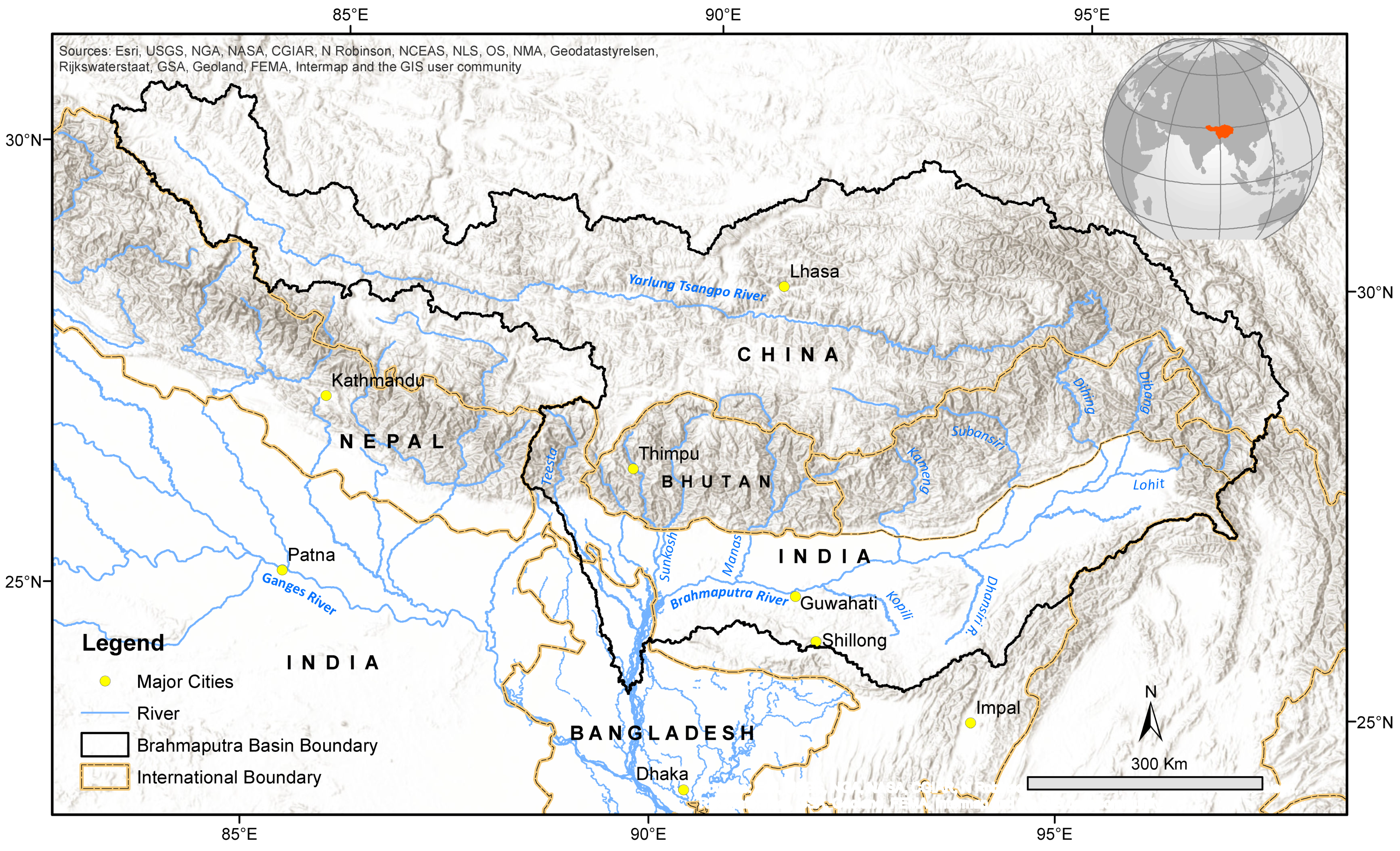
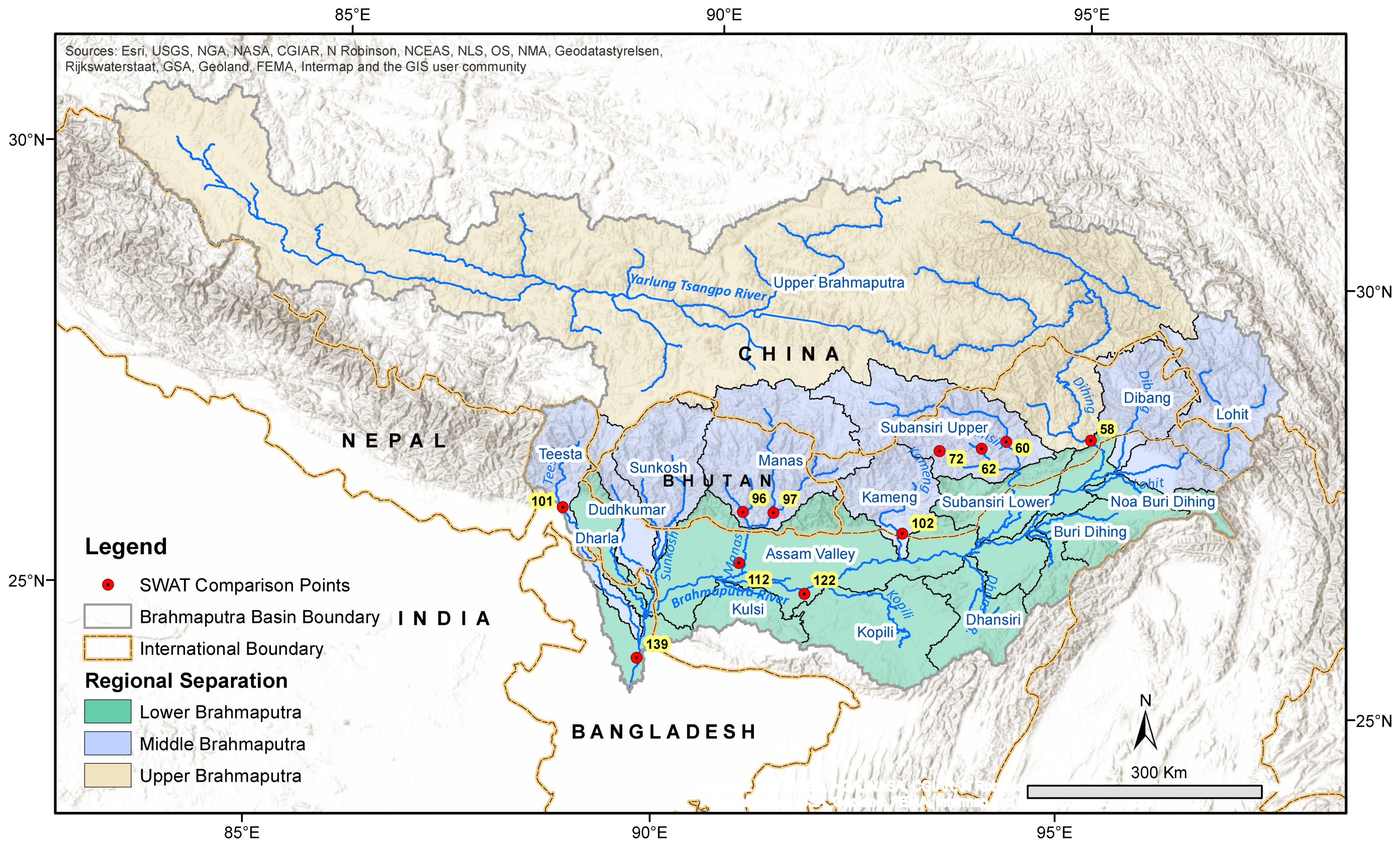
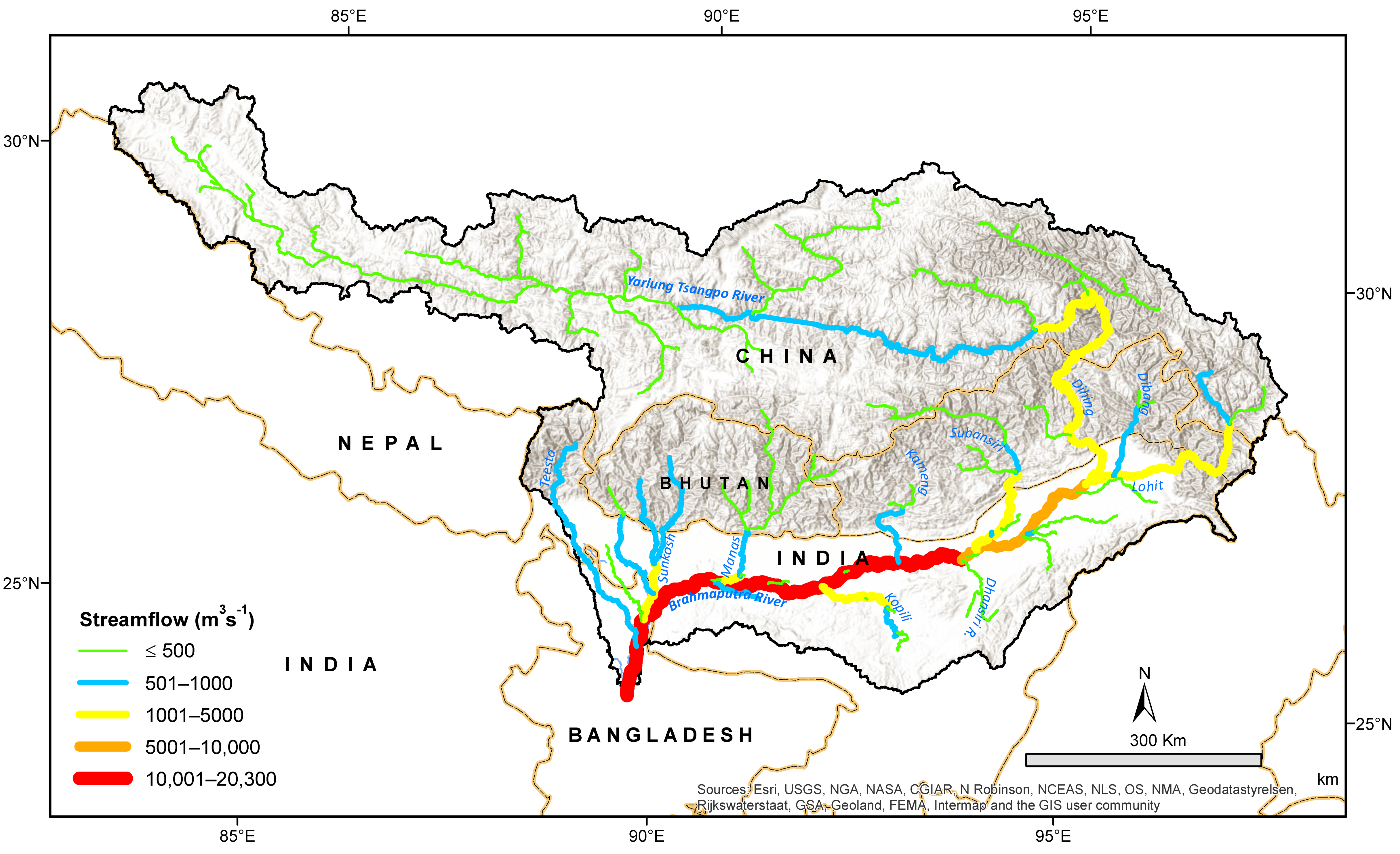
1.2. Study Area
2. Methods and Materials
2.1. Methods
2.2. SWAT Modeling Tool
2.3. Data
2.4. Climate Change Scenarios
2.4.1. Selection of CC Scenarios and GCMs
2.4.2. Generation of Climatic Variables for CC SWAT Simulation
2.5. Statistical Methods for Model Verification
3. Brahmaputra SWAT Model
3.1. Model Development
3.2. Model Calibration and Validation
3.2.1. Simulation, Calibration and Validation Period
3.2.2. Challenge in Model Calibration
3.2.3. Model Parameter Sensitivity Analysis and Calibrated Parameters
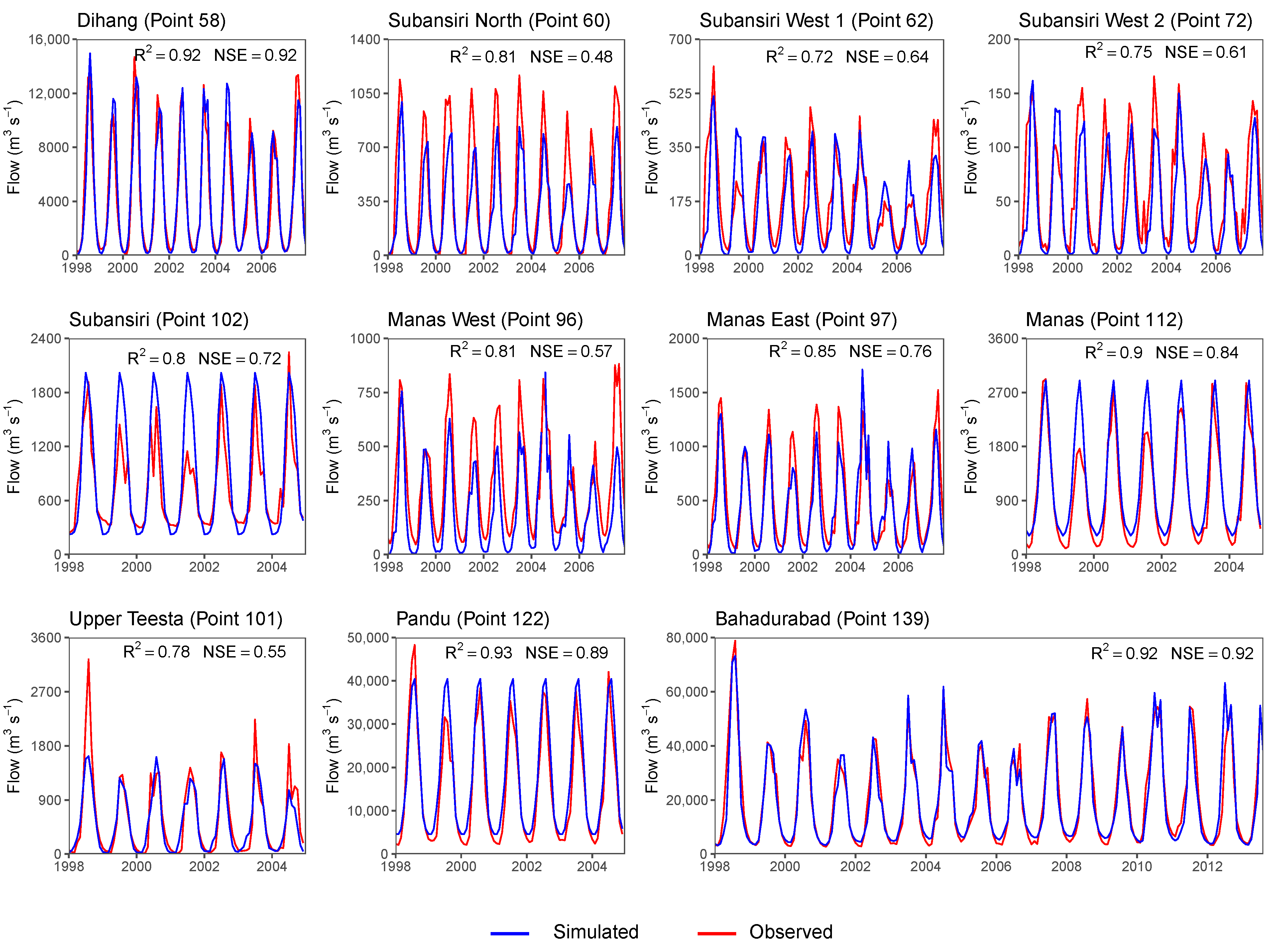
3.3. Model Performance
4. Results and Discussion
4.1. Hydrology and Water Balance
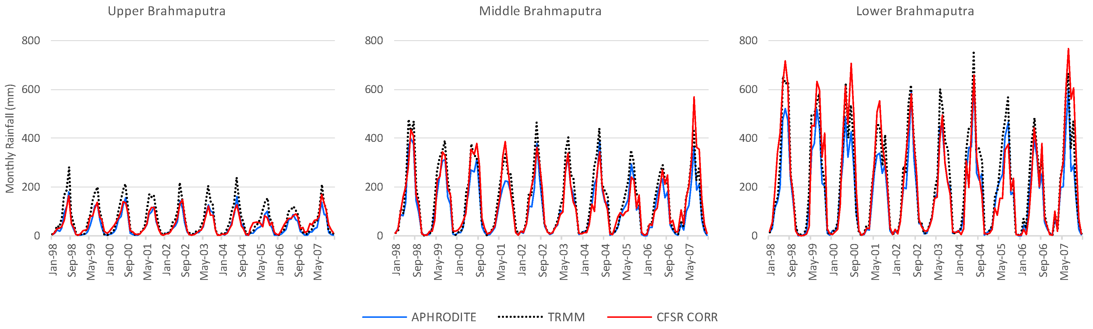
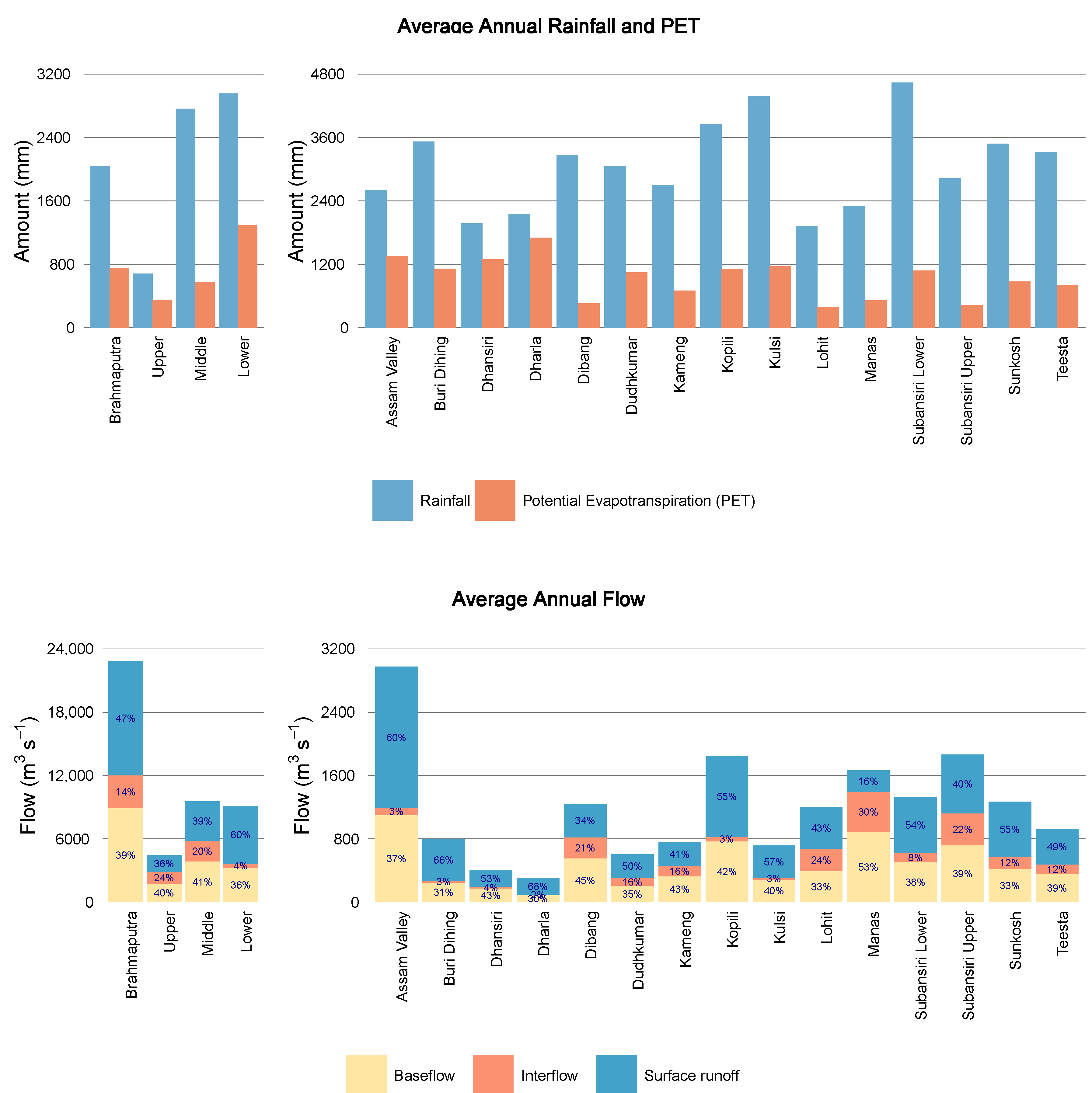
4.1.1. Precipitation and Evapotranspiration
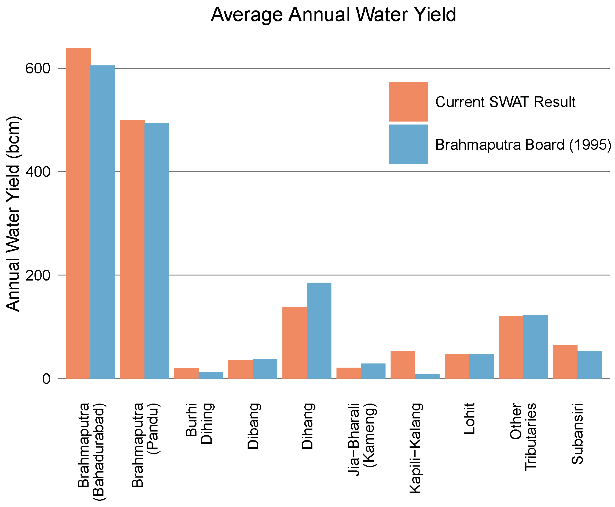
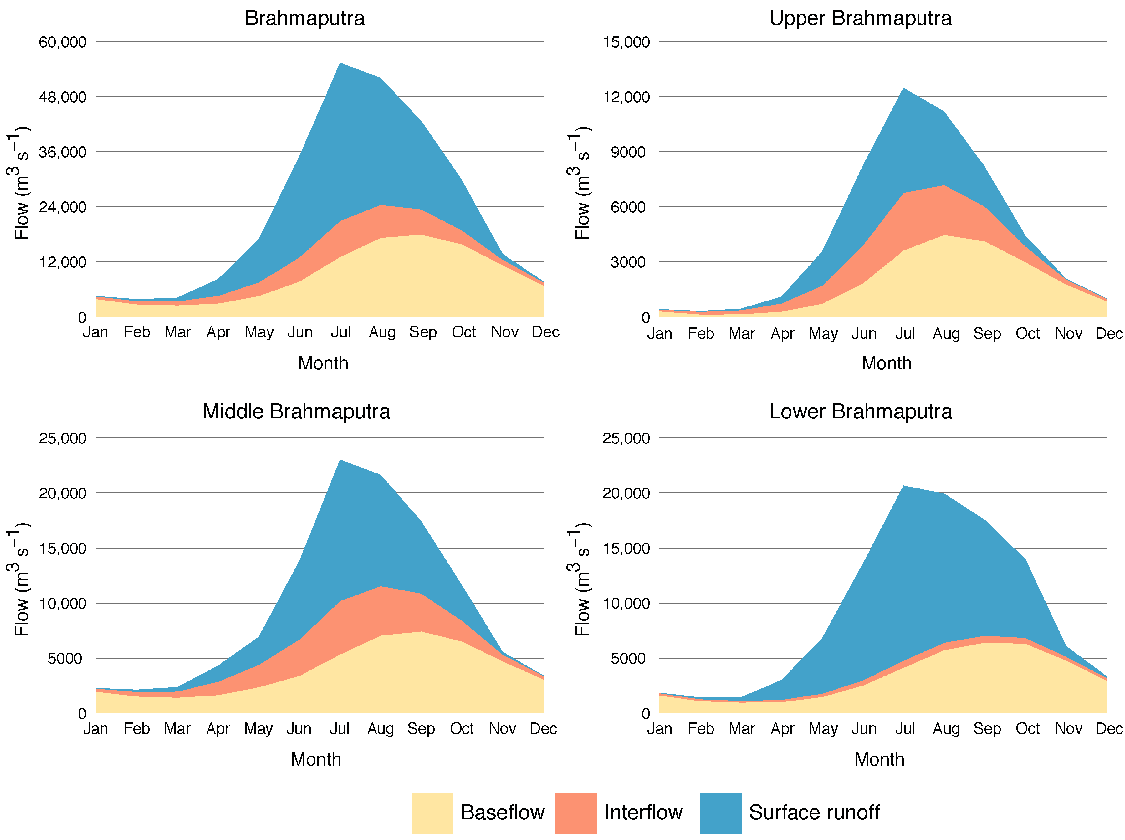
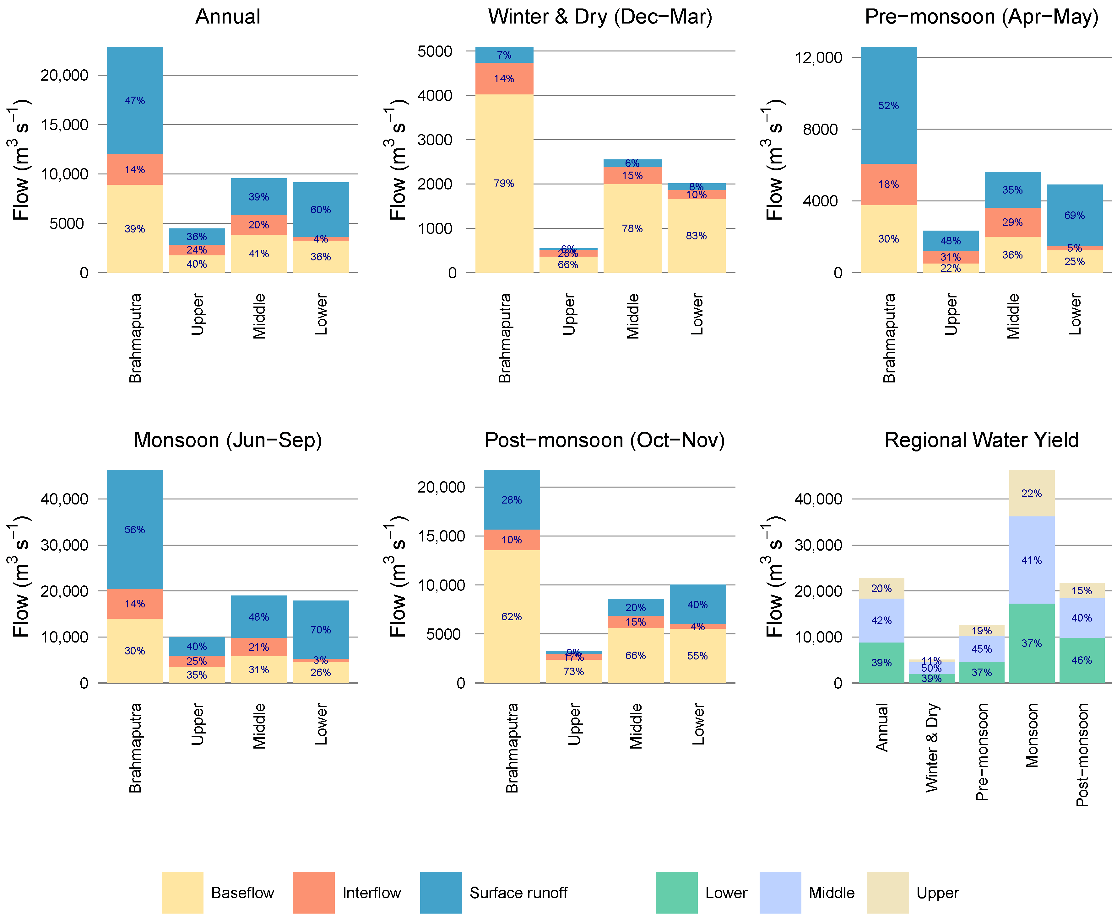
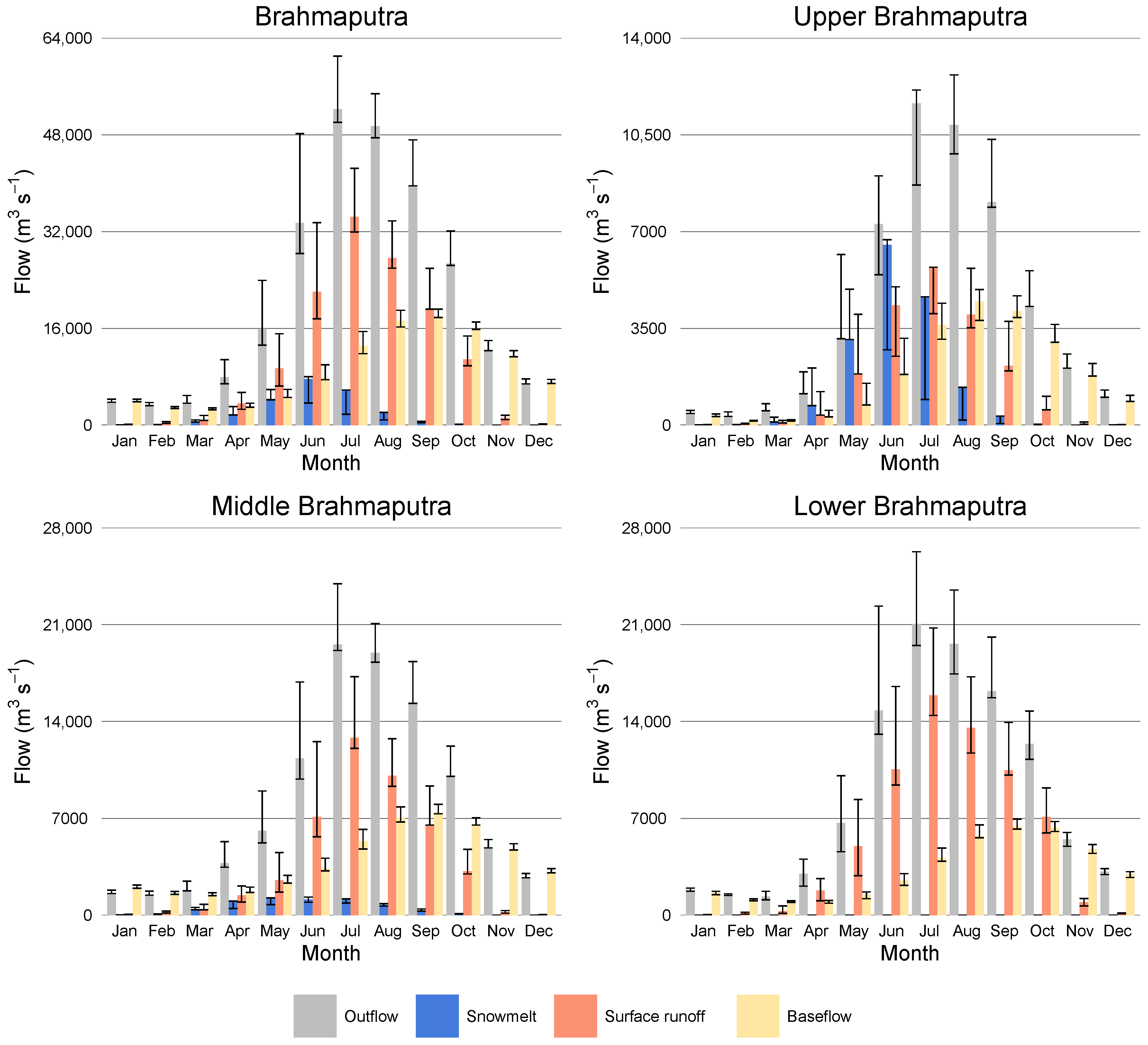
4.1.2. Baseflow, Water Yield and Snowmelt
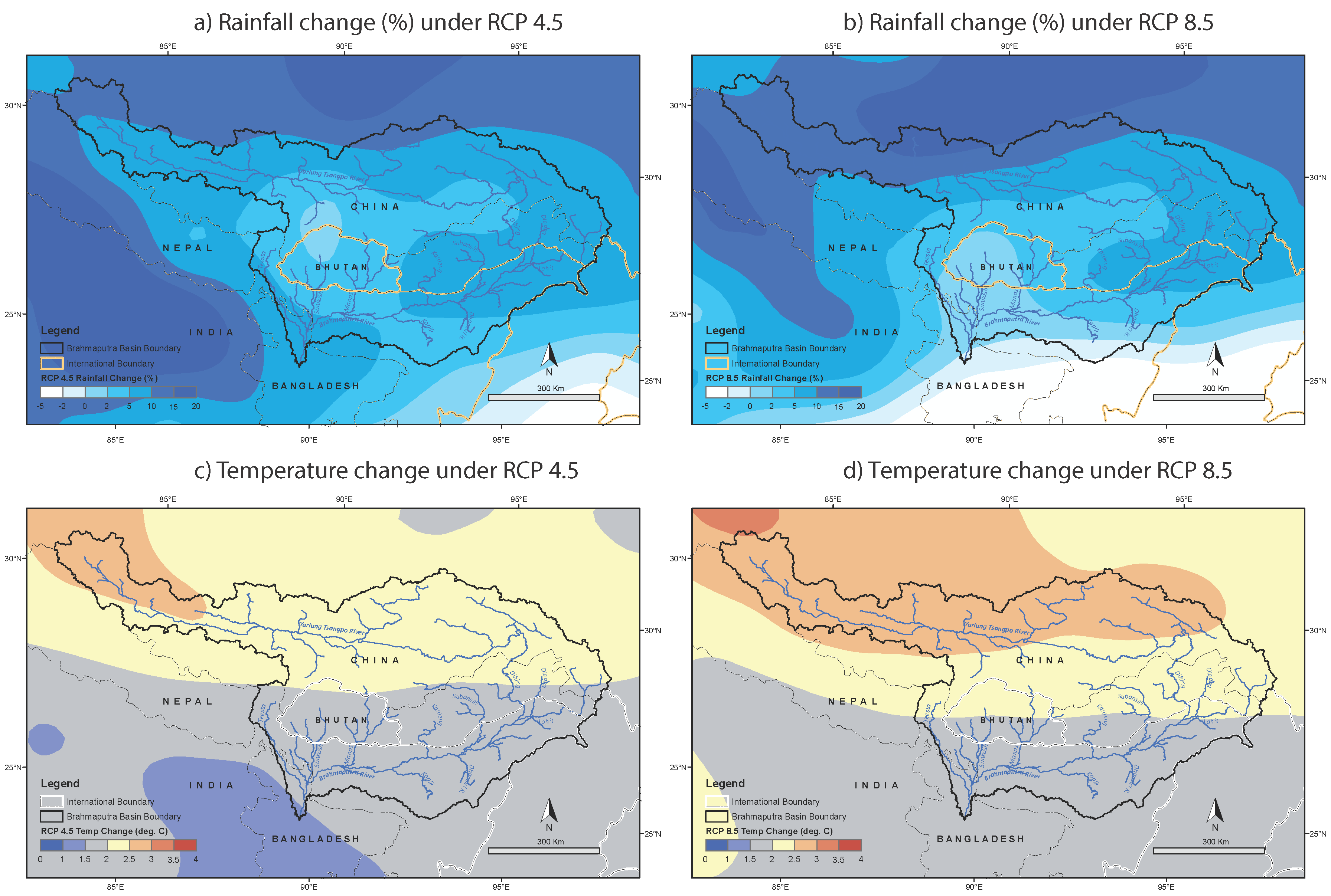
4.2. Impact of Climate Change
5. Conclusions
5.1. Summary of Findings
5.2. Contribution to Basin Water Management
5.3. Limitations
Author Contributions
Funding
Data Availability Statement
Acknowledgments
Conflicts of Interest
References
- Barnett, T.P.; Adam, J.C.; Lettenmaier, D.P. Potential impacts of a warming climate on water availability in snow-dominated regions. Nature 2005, 438, 303–309. [Google Scholar] [CrossRef] [PubMed]
- Viviroli, D.; Dürr, H.H.; Messerli, B.; Meybeck, M.; Weingartner, R. Mountains of the world, water towers for humanity: Typology, mapping, and global significance. Water Resour. Res. 2007, 43, W07447. [Google Scholar] [CrossRef]
- Immerzeel, W.W.; Van Beek, L.P.H.; Konz, M.; Shrestha, A.B.; Bierkens, M.F.P. Hydrological response to climate change in a glacierized catchment in the Himalayas. Clim. Change 2012, 110, 721–736. [Google Scholar] [CrossRef] [PubMed]
- Kaser, G.; Großhauser, M.; Marzeion, B. Contribution potential of glaciers to water availability in different climate regimes. Proc. Natl. Acad. Sci. USA 2010, 107, 20223–20227. [Google Scholar] [CrossRef]
- Cruz, R.V.; Harasawa, H.; Lal, M.; Wu, S. Asia. In Climate Change: Impacts, Adaptation, and Vulnerability; Contribution of Working Group II to the Fourth Assessment Report of the Intergovernmental Panel on Climate Change; Parry, M.L., Canziani, O.F., Palutikof, J.P., Van Der Linden, P.J., Hanson, C.E., Eds.; Cambridge University Press: Cambridge, UK, 2007; pp. 470–506. [Google Scholar]
- Immerzeel, W.; Droogers, P.; de Jong, S.; Bierkens, M. Large-scale monitoring of snow cover and runoff simulation in Himalayan river basins using remote sensing. Remote. Sens. Environ. 2009, 113, 40–49. [Google Scholar] [CrossRef]
- Beniston, M. Climatic Change in Mountain Regions: A Review of Possible Impacts. Clim. Change 2003, 59, 5–31. [Google Scholar] [CrossRef]
- Immerzeel, W.W.; Pellicciotti, F.; Bierkens, M.F.P. Rising river flows throughout the twenty-first century in two Himalayan glacierized watersheds. Nat. Geosci. 2013, 6, 742–745. [Google Scholar] [CrossRef]
- Lutz, A.; Immerzeel, W.; Shrestha, A.B.; Bierkens, M.F. Consistent increase in High Asia’s runoff due to increasing glacier melt and precipitation. Nat. Clim. Change 2014, 4, 587–592. [Google Scholar] [CrossRef]
- Turner, A.G.; Annamalai, H. Climate change and the South Asian summer monsoon. Nat. Clim. Change 2012, 2, 587–595. [Google Scholar] [CrossRef]
- Palash, W.; Quadir, M.E.; Shah-Newaz, S.M.; Kirby, M.D.; Mainuddin, M.; Khan, A.S.; Hossain, M.M. Surface Water Assessment of Bangladesh and Impact of Climate Change. A Supplementary Report of Bangladesh Integrated Water Resources Assessment; Institute of Water Modelling, Bangladesh & Commonwealth Scientific and Industrial Research: Dhaka, Bangladesh, 2014; 150p. [Google Scholar]
- Panday, P.K.; Frey, E.K.; Ghimire, B. Detection of the timing and duration of snowmelt in the Hindu Kush-Himalaya using QuikSCAT, 2000–2008. Environ. Res. Lett. 2011, 6, 24007–24013. [Google Scholar] [CrossRef]
- Jiang, Y.; Palash, W.; Akanda, A.; Small, D.; Islam, S. A Simple Streamflow Forecasting Scheme for the Ganges Basin. In Flood Forecasting; Elsevier Inc.: Amsterdam, The Netherlands, 2016. [Google Scholar] [CrossRef]
- Bolch, T.; Kulkarni, A.; Kääb, A.; Huggel, C.; Paul, F.; Cogley, J.G.; Frey, H.; Kargel, J.S.; Fujita, K.; Scheel, M.; et al. The State and Fate of Himalayan Glaciers. Science 2012, 336, 310–314. [Google Scholar] [CrossRef] [PubMed]
- Akhtar, M.; Ahman, N.; Booij, M.J. Use of regional climate model simulations as input for hydrological models for the Hindukush-Karakorum-Himalaya region. Hydrol. Earth Syst. Sci. 2009, 13, 1075–1089. [Google Scholar] [CrossRef]
- Bharati, L.; Lacombe, G.; Gurung, P.; Jayakody, P.; Hoanh, C.T.; Smakhtin, V. The Impacts of Water Infrastructure and Climate Change on the Hydrology of the Upper Ganges River Basin; IWMI Research Report 142; IWMI: Colombo, Sri Lanka, 2011. [Google Scholar] [CrossRef]
- Gosain, A.K.; Rao, S.; Basuray, D. Climate change impact assessment on the hydrology of Indian river basins. Curr. Sci. 2006, 90, 346–353. [Google Scholar]
- Seidel, K.; Martinec, J.; Baumgartner, M.F. Modelling runoff and impact of climate change in large Himalayan basins. In Proceedings of the International Conference on Integrated Water Resources Management (ICIWRM), Roorkee, India, 19–21 December 2000. [Google Scholar]
- Singh, P.; Haritashya, U.; Kumar, N. Modelling and estimation of different components of streamflow for Gangotri Glacier basin, Himalayas. Hydrol. Sci. J. 2008, 53, 309–322. [Google Scholar] [CrossRef]
- Thomson, A.M.; Calvin, K.V.; Smith, S.J.; Kyle, G.P.; Volke, A.; Patel, P.; Delgado-Arias, S.; Bond-Lamberty, B.; Wise, M.A.; Clarke, L.E.; et al. RCP4.5: A pathway for stabilization of radiative forcing by 2100. Clim. Change 2011, 109, 77–94. [Google Scholar] [CrossRef]
- Sarker, M.H.; Huque, I.; Alam, M.; Koudstaa, R. Rivers, chars, char dwellers of Bangladesh. Int. J. River Basin Manag. 2003, 1, 61–80. [Google Scholar] [CrossRef]
- Palash, W. Hydro-morphological analysis of the Padma-Meghna confluence and its downstream. Master’s Thesis, Katholeike University Leuven, Leuven, Belgium, 2008. [Google Scholar]
- IWM. Water Availability, Demand and Adaptation Option Assessment of the Brahmaputra River Basin under Climate Change; Final Report; ICIMOD: Latipur, Nepal, 2013. [Google Scholar]
- Barman, S.; Bhattacharjya, R.K. Change in snow cover area of Brahmaputra river basin and its sensitivity to temperature. Environ. Syst. Res. 2015, 4, 16. [Google Scholar] [CrossRef]
- Immerzeel, W.; Droogers, P. Calibration of a distributed hydrological model based on satellite evapotranspiration. J. Hydrol. 2008, 349, 411–424. [Google Scholar] [CrossRef]
- Bajracharya, S.R.; Palash, W.; Shrestha, M.S.; Khadgi, V.R.; Duo, C.; Das, P.J.; Dorji, C. Systematic Evaluation of Satellite-Based Rainfall Products over the Brahmaputra Basin for Hydrological Applications. Adv. Meteorol. 2015, 2015, 398687. [Google Scholar] [CrossRef]
- Immerzeel, W.W.; Lutz, A.F. Regional Knowledge Sharing on Climate Change Scenario Downscaling; FutureWater report 116; FutureWater: Wageningen, The Netherlands, 2012; pp. 1–48. [Google Scholar]
- Lutz, A.F.; ter Maat, H.W.; Biemans, H.; Shrestha, A.B.; Wester, P.; Immerzeel, W.W. Selecting representative climate models for climate change impact studies: An advanced envelope-based selection approach. Int. J. Climatol. 2016, 36, 3988–4005. [Google Scholar] [CrossRef]
- Arnold, J.G.; Srinivasan, R.; Muttiah, R.S.; Williams, J.R. Large area hydrologic modeling and assessment. Part I: Model development. J. Am. Water Resour. Assoc. 1998, 34, 73–89. [Google Scholar] [CrossRef]
- Bharati, L.; Jayakody, P. Hydrological impacts of inflow and land-use changes in the Gorai River catchment, Bangladesh. Water Int. 2011, 36, 357–369. [Google Scholar] [CrossRef]
- Daniel, E.B.; Camp, J.V.; LeBoeuf, E.; Penrod, J.; Dobbins, J.; Abkowitz, M.D. Watershed Modeling and its Applications: A State-of-the-Art Review. Open Hydrol. J. 2011, 5, 26–50. [Google Scholar] [CrossRef]
- Garg, K.K.; Karlberg, L.; Barron, J.; Wani, S.P.; Rockstrom, J. Assessing the impacts of agricultural interventions in the Kothapally watershed, Southern India. Hydrol. Process. 2012, 26, 387–404. [Google Scholar] [CrossRef]
- Jha, M.K. Evaluating Hydrologic Response of an Agricultural Watershed for Watershed Analysis. Water 2011, 3, 604–617. [Google Scholar] [CrossRef]
- Pilling, C.G.; Jones, J.A.A. The impact of future climate change on seasonal discharge, hydrological processes and extreme flows in the Upper Wye experimental catchment, Mid-Wales. Hydrol. Process. 2002, 16, 1201–1213. [Google Scholar] [CrossRef]
- Srinivasan, R.; Ramanarayanan, T.S.; Arnold, J.G.; Bednarz, S.T. Large area hydrologic modeling and assessment part ii: Model application. JAWRA J. Am. Water Resour. Assoc. 1998, 34, 91–101. [Google Scholar] [CrossRef]
- Biesbrouck, B.; Wyseure, G.; Van Orschoven, J.; Feyen, J. AVSWAT2000; Course; Catholic University of Leuven, Laboratory for Soil and Water Management (LSWM): Leuven, Belgium, 2002. [Google Scholar]
- Di Luzio, M.; Srinivasan, R.; Arnold, J.G. Integration of watershed tools and swat model into basins. JAWRA J. Am. Water Resour. Assoc. 2002, 38, 1127–1141. [Google Scholar] [CrossRef]
- Neitsch, S.L.; Arnold, J.G.; Kiniry, J.R.; Williams, J.R. Soil and Water Assessment Tool—Theoretical Documentation (version 2009); Grassland, Soil and Water Research Laboratory, Agricultural Research Service, Blackland Research Center, Texas Agricultural Experiment Station: Temple, TX, USA, 2011. [Google Scholar]
- Wang, X.; Melesse, A.M. Evaluation of the swat model’s snowmelt hydrology in a northwestern minnesota watershed. Trans. ASAE 2005, 48, 1359–1376. [Google Scholar] [CrossRef]
- Lévesque, É.; Anctil, F.; Van Griensven, A.; Beauchamp, N. Evaluation of streamflow simulation by SWAT model for two small watersheds under snowmelt and rainfall. Hydrol. Sci. J. 2008, 53, 961–976. [Google Scholar] [CrossRef]
- Omani, N.; Srinivasan, R.; Smith, P.K.; Karthikeyan, R. Glacier mass balance simulation using SWAT distributed snow algorithm. Hydrol. Sci. J. 2016, 62, 546–560. [Google Scholar] [CrossRef]
- Rahman, K.; Maringanti, C.; Beniston, M.; Widmer, F.; Abbaspour, K.; Lehmann, A. Streamflow Modeling in a Highly Managed Mountainous Glacier Watershed Using SWAT: The Upper Rhone River Watershed Case in Switzerland. Water Resour. Manag. 2013, 27, 323–339. [Google Scholar] [CrossRef]
- Jarvis, A.; Reuter, H.I.; Nelson, A.; Guevara, E. Hole-filled SRTM for the globe Version 4. CGIAR-CSI SRTM 90m Database. 2008. Available online: http://srtm.csi.cgiar.org (accessed on 1 May 2020).
- Arino, O.; Ramos, J.; Kalogirou, V.; Defourny, P.; Achard, F. GlobCover 2009. Available online: https://epic.awi.de/id/eprint/31045/1/2017278_arino_poster.pdf (accessed on 29 November 2022).
- FAO; IIASA; ISRIC; ISSCAS; JRC. Harmonized World Soil Database (version 1.2); FAO: Rome, Italy; IIASA: Laxenburg, Austria, 2012. [Google Scholar]
- Saha, S. NCEP Climate Forecast System Reanalysis (CFSR) Selected Hourly Time-Series Products, January 1979 to December 2010. Bull. Amer. Meteor. Soc. 2010, 91, 1015–1057. [Google Scholar] [CrossRef]
- Dile, Y.T.; Srinivasan, R. Evaluation of CFSR climate data for hydrologic prediction in data-scarce watersheds: An application in the Blue Nile River Basin. JAWRA J. Am. Water Resour. Assoc. 2014, 50, 1226–1241. [Google Scholar] [CrossRef]
- Fuka, D.R.; Walter, M.T.; MacAlister, C.; DeGaetano, A.T.; Steenhuis, T.S.; Easton, Z.M. Using the Climate Forecast System Reanalysis as weather input data for watershed models. Hydrol. Process. 2013, 28, 5613–5623. [Google Scholar] [CrossRef]
- Hall, D.; Salomonson, V.V.; George, K. MODIS/Terra Snow Cover Monthly L3 Global 0.05Deg CMG; Version 5; NSIDC, National Snow and Ice Data Center: Boulder, CO, USA, 2006. [Google Scholar] [CrossRef]
- Tedesco, M.; Kelly, R.; Foster, J.L.; Chang, A.T.C. AMSR-E/Aqua Monthly L3 Global Snow Water Equivalent EASE-Grid; Version 2; NASA National Snow and Ice Data Center Distributed Active Archive Center: Boulder, CO, USA, 2004. [CrossRef]
- Lutz, A.F.; Immerzeel, W.W. Water Availability Analysis for the Upper Indus, Ganges, Brahmaputra, Salween and Mekong River Basins, Final Report. FutureWater report 127; FutureWater: Wageningen, The Netherlands, 2013; pp. 1–83. [Google Scholar]
- Déqué, M.; Rowell, D.P.; Lüthi, D.; Giorgi, F.; Christensen, J.H.; Rockel, B.; Jacob, D.; Kjellström, E.; de Castro, M.; Hurk, B.V.D. An intercomparison of regional climate simulations for Europe: Assessing uncertainties in model projections. Clim. Change 2007, 81, 53–70. [Google Scholar] [CrossRef]
- Moss, R.H.; Edmonds, J.A.; Hibbard, K.A.; Manning, M.R.; Rose, S.K.; Van Vuuren, D.P.; Carter, T.R.; Emori, S.; Kainuma, M.; Kram, T. The next generation of scenarios for climate change research and assessment. Nature 2010, 463, 747–756. [Google Scholar] [CrossRef]
- Stocker, T.F.; Qin, D.; Plattner, G.-K.; Tignor, M.; Allen, S.K.; Boschung, J.; Nauels, A.; Xia, Y.; Bex, V.; Midgley, P.M. (Eds.) The Physical Science Basis. Contribution of Working Group I to the Fifth Assessment Report of the Intergovernmental Panel on Climate Change; IPCC; Cambridge University Press: Cambridge, UK; New York, NY, USA, 2013; 1535p. [Google Scholar]
- Rajbhandari, R.; Shrestha, A.B.; Nepal, S.; Wahid, S. Projection of future climate over the Koshi River basin based on CMIP5 GCMs. Atmospheric Clim. Sci. 2016, 6, 190–204. [Google Scholar] [CrossRef]
- Arnell, N.W. The effect of climate change on hydrological regimes in Europe: A continental perspective. Glob. Environ. Change 1999, 9, 5–23. [Google Scholar] [CrossRef]
- Kay, A.L.; Davies, H.N.; Bell, V.A.; Jones, R.G. Comparison of uncertainty sources for climate change impacts: Flood frequency in England. Clim. Change 2009, 92, 41–63. [Google Scholar] [CrossRef]
- Gupta, H.V.; Sorooshian, S.; Yapo, P.O. Status of automatic calibration for hydrologic models: Comparison with multilevel expert calibration. J. Hydrologic Eng. 1999, 4, 135–143. [Google Scholar] [CrossRef]
- Moriasi, D.N.; Arnold, J.G.; van Liew, M.W.; Bingner, R.L.; Harmel, R.D.; Veith, T.L. Model Evaluation Guidelines for Systematic Quantification of Accuracy in Watershed Simulations. Trans. ASABE 2007, 50, 885–900. Available online: http://swat.tamu.edu/media/1312/moriasimodeleval.pdf (accessed on 20 August 2020). [CrossRef]
- Singh, J.; Knapp, H.V.; Demissie, M. Hydrologic Modeling of the Iroquois River Watershed Using HSPF and SWAT; ISWS CR 2004-08; Illinois State Water Survey: Champaign, IL, USA, 2004; Available online: www.sws.uiuc.edu/pubdoc/CR/ (accessed on 20 August 2020).
- Mahanta, C.; Zaman, A.M.; Shah-Newaz, S.M.; Rahman, S.M.; Mazumdar, T.K.; Choudhury, R.; Borah, P.J.; Saikia, L. Physical Assessment of the Brahmaputra River; IUCN, The International Union for Conservation of Nature: Dhaka, Bangladesh, 2014. [Google Scholar]
- Immerzeel, W.W.; Van Beek, L.P.H.; Bierkens, M.F.P. Climate change will affect the Asian water towers. Science 2010, 328, 1382–1385. [Google Scholar] [CrossRef] [PubMed]
- Yang, Y.E.; Wi, S.; Ray, P.A.; Brown, C.M.; Khalil, A.F. The future nexus of the Brahmaputra River Basin: Climate, water, energy and food trajectories. Glob. Environ. Change 2016, 37, 16–30. [Google Scholar] [CrossRef]
- Alley, K.D.; Hile, R.; Mitra, C. Visualizing Hydropower Across the Himalayas: Mapping in a time of Regulatory Decline, Himalaya. J. Assoc. Nepal Himal. Stud. 2014, 34, 9. [Google Scholar]
- McCully, P. Silenced Rivers, The Ecology and Politics of Large Dams; Zed Books: London, UK, 1996. [Google Scholar]
- Samaranayake, N.; Limaye, S.; Wuthnow, J. Water Resource Competition in the Brahmaputra River Basin; CNA Analysis and Solutions: Arlington, VI, USA, 2016. [Google Scholar]
- Islam, S.; Susskind, L. Water Diplomacy: A Negotiated Approach to Managing Complex Water Networks; Routledge: New York, NY, USA, 2012. [Google Scholar]


| Data Type | Source | Spatial Resolution | Temporal Resolution |
|---|---|---|---|
| Digital elevation model (DEM) | SRTM | 90 m | |
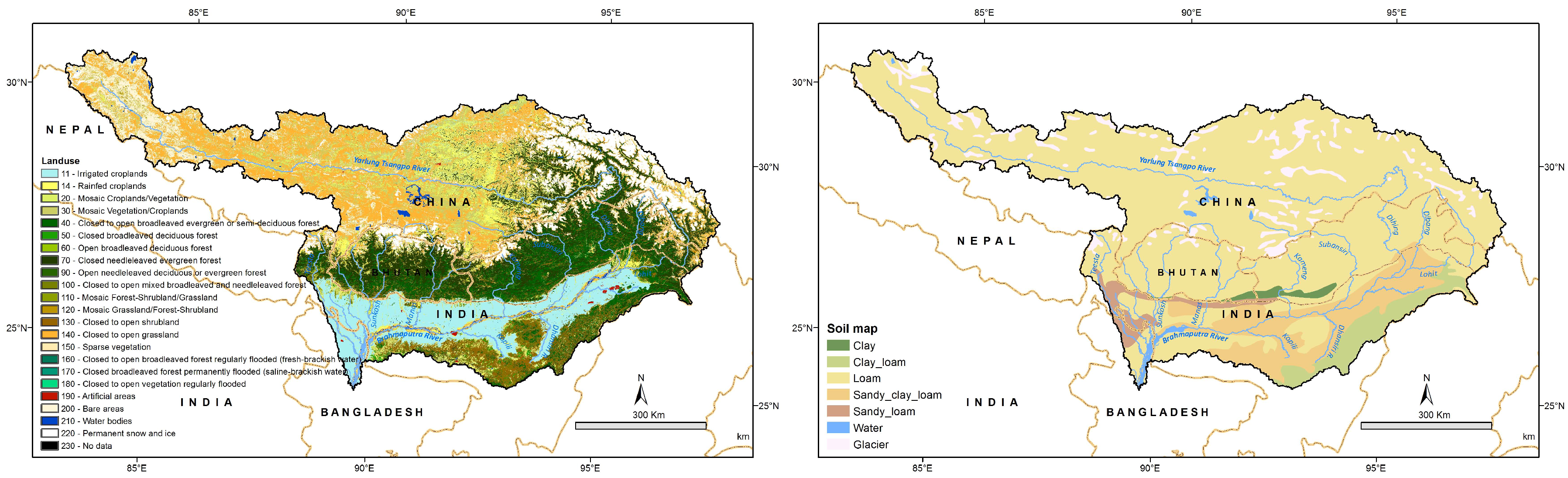
| Land use | GlobCover 2009 V2.3 | 1/360° | |
| Soil class map | Harmonized World Soil Database V1.2 | 1/120° | |
| Hydro-meteorological data (rainfall, temperature, relative humidity, solar radiation, wind speed) | Climate Forecast System Reanalysis (CFSR) | 0.5° | Daily |
| Weather generator data | Climate Forecast System Reanalysis (CFSR) | 0.5° | Historical analysis |
| Monthly snow cover data | MODIS/Terra Snow Cover Monthly L3 Global CMG, V5.0 | 0.5° | Monthly |
| Monthly snow water equivalent | AMSR-E/Aqua Monthly L3 Global Snow Water Equivalent EASE-Grids, V2.0 | 25 km | Monthly |
| Streamflow observations | BWDB, RivDis, ICIMOD, Immerzeel et al., [8] | Daily |
| River Point | Location Name | Longitude (deg.) | Latitude (deg.) | Upstream Sub-Basin Name | Data Type | Available Data Period | Data Source |
|---|---|---|---|---|---|---|---|
| 58 | Dihang | 91.88 | 29.28 | All Tibetan sub-basins in the upper Brahmaputra | Simulated results from HI-SPHY model | 1956―1982 | RivDis |
| 60 | 94.15 | 28.08 | Upper Subansiri | 1998―2007 | Lutz and Immerzeel [51] | ||
| 62 | 93.84 | 27.98 | Middle Subansiri 1 | ||||
| 72 | 93.30 | 27.92 | Middle Subansiri 2 | ||||
| 96 | 90.84 | 27.01 | Manas West | ||||
| 97 | 91.23 | 27.03 | Manas East | ||||
| 101 | Anderson Bridge | 88.54 | 26.82 | Upper Teesta | |||
| 102 | Jai Bhorelli | 92.89 | 26.93 | Kameng | Measured | 1958―1979 | RivDis |
| 112 | Manas | 90.84 | 26.41 | Manas (upper and lower) | 1955―1974 | ||
| 122 | Pandu | 91.70 | 26.13 | Upper Brahmaputra, Dibang, Lohit, Subansiri, Kameng, Buri Dihing, Dhansiri, upper Assam Valley | 1956―1979 | ||
| 139 | Bahadurabad | 89.66 | 25.18 | Whole Brahmaputra | 1979―2014 | BWDB |
| Model Number | Selected Model | Climate Type | RCP | ∆P (% change) | ∆T (°C anomaly) | Source |
|---|---|---|---|---|---|---|
| 1 | GISS-E2-R-r4i1p1_rcp45 | DRY, COLD | RCP 4.5 | 4.8 | 1.4 | Goddard Institute for Space Studies, NOAA, USA |
| 2 | IPSL-CM5A-LR-r4i1p1_rcp45 | DRY, WARM | 7.2 | 2.0 | Institut Pierre Simon Laplace, France | |
| 3 | IPSL-CM5A-LR-r3i1p1_rcp45 | WET, COLD | 6.7 | 2.4 | Institut Pierre Simon Laplace, France | |
| 4 | CanESM2-r4i1p1_rcp45 | WET, WARM | 11.4 | 2.3 | Canadian Centre for Climate Modelling and Analysis, Canada | |
| 5 | GFDL-ESM2G-r1i1p1_rcp85 | DRY, COLD | RCP 8.5 | 7.3 | 1.7 | Geophysical Fluid Dynamics Laboratory, NOAA, USA |
| 6 | IPSL-CM5A-LR-r4i1p1_rcp85 | DRY, WARM | −5.5 | 2.8 | Institut Pierre Simon Laplace, France | |
| 7 | CSIRO-Mk3-6-0-r3i1p1_rcp85 | WET, COLD | 12.6 | 1.7 | Commonwealth Scientific and Industrial Research Organisation, Australia | |
| 8 | CanESM2-r4i1p1_rcp85 | WET, WARM | 12.1 | 2.8 | Canadian Centre for Climate Modelling and Analysis, Canada |
| Parameter | Value Range | Upper Brahmaputra | Middle Brahmaputra | Lower Brahmaputra | |
|---|---|---|---|---|---|
| CN2 | 35–98 | 70–87 | 53–87 | 73–84 |  |
| GW_DELAY (Days) | 0–500 | 31 | 31–385 | 31–385 | |
| ALPHA_BF | 0–1 | 0.05 | 0.05–0.81 | 0.05–0.81 | |
| GWQMN (mm) | 0–500 | 1000 | 1000 | 1000 | |
| PLAPS (mm/km) | −1000–1000 | −200 | −200 | - | |
| TLAPS (°C/km) | −10–10 | −6.5 | −6.5 | - | |
| SOL_BD (g/cc) | 0.9–2.5 | 1–1.5 | 1–1.5 | - | |
| SFTMP (°C) | −5–5 | 2 | 2 | - | |
| SMTMP (°C) | −5–5 | 2 | 2 | - | |
| SMFMX (mm H2O/°C-day) | 0–4.5 | 1.5 | 1.5 | - | |
| SMFMN (mm H2O/°C-day) | 0–4.5 | 0.5 | 0.5 | - | |
| TIMP | 0–1 | 0.5 | 0.5 | - | |
| SNOCOVMX (mm) | 0–500 | 200 | 200 | - | |
| SNO50COV (%) | 0–1 | 0.65 | 0.65 | - |
| River Name (Point No.) | Performance Statistics | |||||||||
|---|---|---|---|---|---|---|---|---|---|---|
| Peak Obs. Value (m3s−1) | Peak Sim. Value (m3s−1) | Peak Error (m3s−1) | Mean Error (ME) (m3s−1) | Mean Abs. Error (MAE) (m3s−1) | RMSE (m3s−1) | R2 | NSE | PBIAS (%) | RSR | |
| Dihang (58) | 14,969 | 14,680 | 289 | 21 | 142 | 1326 | 0.90 | 0.90 | 2.9 | 0.32 |
| Subansiri North (60) | 994 | 1166 | −172 | −16 | 20 | 192 | 0.83 | 0.48 | 35.1 | 0.72 |
| Subansiri West 1 (62) | 516 | 613 | −97 | −6 | 10 | 82 | 0.70 | 0.62 | 24.1 | 0.62 |
| Subansiri West 2 (72) | 162 | 166 | −4 | −3 | 3 | 28 | 0.76 | 0.60 | 36.1 | 0.63 |
| Manas West (96) | 1205 | 882 | 323 | −18 | 21 | 158 | 0.75 | 0.46 | 51.7 | 0.73 |
| Manas East (97) | 1712 | 1523 | 189 | −11 | 24 | 188 | 0.82 | 0.75 | 16.1 | 0.49 |
| Upper Teesta (101) | 1631 | 3239 | −1608 | −8 | 30 | 315 | 0.78 | 0.55 | 9.9 | 0.67 |
| Kameng (102) | 2019 | 2247 | −228 | 33 | 46 | 438 | 0.67 | 0.55 | 23.2 | 0.67 |
| Manas (112) | 2899 | 2924 | −25 | 44 | 53 | 471 | 0.81 | 0.72 | 22.3 | 0.53 |
| Brahmaputra at Pandu (122) | 40,439 | 48,320 | −7881 | 619 | 718 | 6191 | 0.86 | 0.77 | 21.0 | 0.47 |
| Brahmaputra at Bahadurabad (139) | 73,266 | 78,910 | −5644 | −108 | 822 | 4889 | 0.92 | 0.92 | 2.1 | 0.29 |
| Name | Outflow (m3s−1) | Total Precipitation (mm) | Total AET (mm) | Soil Water (mm) | Snowmelt (m3s−1) | Surface Runoff (m3s−1) | Baseflow (m3s−1) | Interflow (m3s−1) | Water Yield (m3s−1) | Snowmelt to Runoff (m3s−1) |
|---|---|---|---|---|---|---|---|---|---|---|
| Brahmaputra | 21,262 | 2039 | 377 | 142 | 1911 | 10,805 | 8903 | 3122 | 22,829 | 1253 |
| Upper Brahmaputra | 4226 | 684 | 114 | 153 | 1402 | 1595 | 1775 | 1082 | 4452 | 870 |
| Middle Brahmaputra | 8122 | 2859 | 364 | 137 | 510 | 3714 | 3873 | 1949 | 9536 | 383 |
| Lower Brahmaputra | 8913 | 2837 | 684 | 120 | - | 5495 | 3255 | 381 | 8841 | - |
| Assam Valley | 19,893 | 2605 | 682 | 135 | - | 1775 | 1101 | 95 | 2971 | - |
| Buri Dihing | 676 | 3519 | 593 | 68 | - | 524 | 249 | 24 | 797 | - |
| Dhansiri | 382 | 1975 | 712 | 94 | - | 215 | 174 | 17 | 406 | - |
| Dharla | 301 | 2153 | 645 | 123 | - | 205 | 91 | 7 | 303 | - |
| Dibang | 1228 | 3270 | 332 | 121 | 121 | 423 | 555 | 266 | 1245 | 76 |
| Dikhu | 125 | 1676 | 594 | 57 | - | 53 | 57 | 16 | 126 | - |
| Dudhkumar | 603 | 3052 | 490 | 93 | - | 300 | 209 | 96 | 604 | - |
| Kameng | 724 | 2697 | 464 | 169 | 16 | 309 | 329 | 124 | 761 | 14 |
| Kopili | 1802 | 3854 | 754 | 150 | - | 1022 | 771 | 53 | 1847 | - |
| Kulsi | 716 | 4377 | 760 | 164 | - | 408 | 287 | 21 | 717 | - |
| Lohit | 1485 | 1921 | 176 | 188 | 208 | 520 | 393 | 283 | 1195 | 173 |
| Manas | 875 | 2309 | 236 | 115 | 46 | 274 | 887 | 505 | 1667 | 31 |
| Noa Buri Dihing | 65 | 1117 | 620 | 120 | - | 36 | 24 | 7 | 66 | - |
| Lower Subansiri | 2729 | 4634 | 671 | 154 | - | 712 | 507 | 111 | 1331 | - |
| Upper Subansiri | 1178 | 2826 | 318 | 145 | 105 | 743 | 720 | 403 | 1866 | 75 |
| Sunkosh | 1179 | 3479 | 422 | 158 | 5 | 692 | 419 | 158 | 1268 | 4 |
| Teesta | 850 | 3318 | 472 | 105 | 8 | 453 | 361 | 115 | 929 | 9 |
| Name | Season | Outflow (m3s−1) | Total Precipitation (mm) | Total AET (mm) | Snowmelt (m3s−1) | Surface Runoff (m3s−1) | Baseflow (m3s−1) | Interflow (m3s−1) | Water Yield (m3s−1) | Snowmelt to Runoff (m3s−1) |
|---|---|---|---|---|---|---|---|---|---|---|
| Brahmaputra | Winter and Dry | 4384 | 388 | 144 | 150 | 348 | 4027 | 712 | 5087 | 94 |
| Pre-monsoon | 11,906 | 1979 | 579 | 3012 | 6489 | 3770 | 2311 | 12,569 | 1311 | |
| Monsoon | 43,662 | 4189 | 569 | 4048 | 25,802 | 14,016 | 6443 | 46,261 | 2965 | |
| Post-monsoon | 19,573 | 1100 | 259 | 60 | 6039 | 13,562 | 2110 | 21,712 | 87 | |
| Upper Brahmaputra | Winter and Dry | 565 | 354 | 31 | 32 | 33 | 364 | 153 | 550 | 3 |
| Pre-monsoon | 2131 | 722 | 123 | 1902 | 1106 | 511 | 711 | 2329 | 660 | |
| Monsoon | 9459 | 1145 | 209 | 3215 | 4049 | 3514 | 2455 | 10,018 | 2269 | |
| Post-monsoon | 3178 | 384 | 82 | 15 | 298 | 2385 | 567 | 3250 | 15 | |
| Middle Brahmaputra | Winter and Dry | 1870 | 529 | 157 | 118 | 161 | 1997 | 392 | 2549 | 90 |
| Pre-monsoon | 4943 | 2386 | 592 | 1110 | 1984 | 2010 | 1617 | 5612 | 651 | |
| Monsoon | 16,291 | 6137 | 511 | 833 | 9136 | 5804 | 4023 | 18,963 | 696 | |
| Post-monsoon | 7466 | 1436 | 256 | 45 | 1709 | 5623 | 1246 | 8578 | 72 | |
| Lower Brahmaputra | Winter and Dry | 1948 | 250 | 240 | - | 154 | 1666 | 197 | 1987 | - |
| Pre-monsoon | 4833 | 2759 | 1041 | - | 3398 | 1248 | 253 | 4629 | - | |
| Monsoon | 17,912 | 6077 | 1056 | - | 12,617 | 4698 | 602 | 17,280 | - | |
| Post-monsoon | 8929 | 1614 | 473 | - | 4032 | 5555 | 434 | 9884 | - |
Disclaimer/Publisher’s Note: The statements, opinions and data contained in all publications are solely those of the individual author(s) and contributor(s) and not of MDPI and/or the editor(s). MDPI and/or the editor(s) disclaim responsibility for any injury to people or property resulting from any ideas, methods, instructions or products referred to in the content. |
© 2023 by the authors. Licensee MDPI, Basel, Switzerland. This article is an open access article distributed under the terms and conditions of the Creative Commons Attribution (CC BY) license (https://creativecommons.org/licenses/by/4.0/).
Share and Cite
Palash, W.; Bajracharya, S.R.; Shrestha, A.B.; Wahid, S.; Hossain, M.S.; Mogumder, T.K.; Mazumder, L.C. Climate Change Impacts on the Hydrology of the Brahmaputra River Basin. Climate 2023, 11, 18. https://doi.org/10.3390/cli11010018
Palash W, Bajracharya SR, Shrestha AB, Wahid S, Hossain MS, Mogumder TK, Mazumder LC. Climate Change Impacts on the Hydrology of the Brahmaputra River Basin. Climate. 2023; 11(1):18. https://doi.org/10.3390/cli11010018
Chicago/Turabian StylePalash, Wahid, Sagar Ratna Bajracharya, Arun Bhakta Shrestha, Shahriar Wahid, Md. Shahadat Hossain, Tarun Kanti Mogumder, and Liton Chandra Mazumder. 2023. "Climate Change Impacts on the Hydrology of the Brahmaputra River Basin" Climate 11, no. 1: 18. https://doi.org/10.3390/cli11010018
APA StylePalash, W., Bajracharya, S. R., Shrestha, A. B., Wahid, S., Hossain, M. S., Mogumder, T. K., & Mazumder, L. C. (2023). Climate Change Impacts on the Hydrology of the Brahmaputra River Basin. Climate, 11(1), 18. https://doi.org/10.3390/cli11010018