
Role of Metaheuristic Approaches for Implementation of Integrated MPPT-PV Systems: A Comprehensive Study
 , , , and
Abstract
:1. Introduction
- More efficiency;
- Capability of optimizing voltage differences as well as DC load optimization;
- Best for larger systems where solar panel output exceeds battery voltage by a significant margin;
- Enhances the system’s output and hence its capacity.
- Ease of representation: In distinct sections, the work summarizes the main characteristics of traditional and AI-based metaheuristic techniques in a simplified style using simplified flowcharts;
- Ease of analysis: A technical datasheet was created after reviewing all the major attributes required to design any PV system of recently reported conventional MPPT techniques, AI-based metaheuristic approaches, and other AI-based MPPT techniques. This datasheet provides a bare-bones description that facilitates even a new learner to understand the performances of these metaheuristic MPPT techniques, particularly PV systems in PSCs;
- Ease of modification: The technical datasheet highlights the pros and cons of all reviewed works of each category, which enables the user to identify the research gap as discussed above and helps them to modify a particular algorithm to meet the requirement of good PV system;
- Qualitative comparative analysis: The technical datasheet facilitates comparison of all MPPT approaches based on the key characteristics required while incorporating them in any PV system, which helps the readers to select the most suitable technique for any particular application.
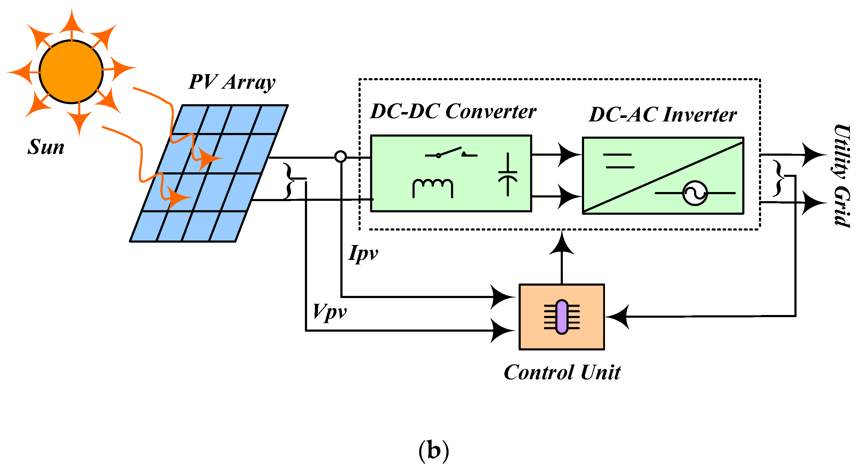
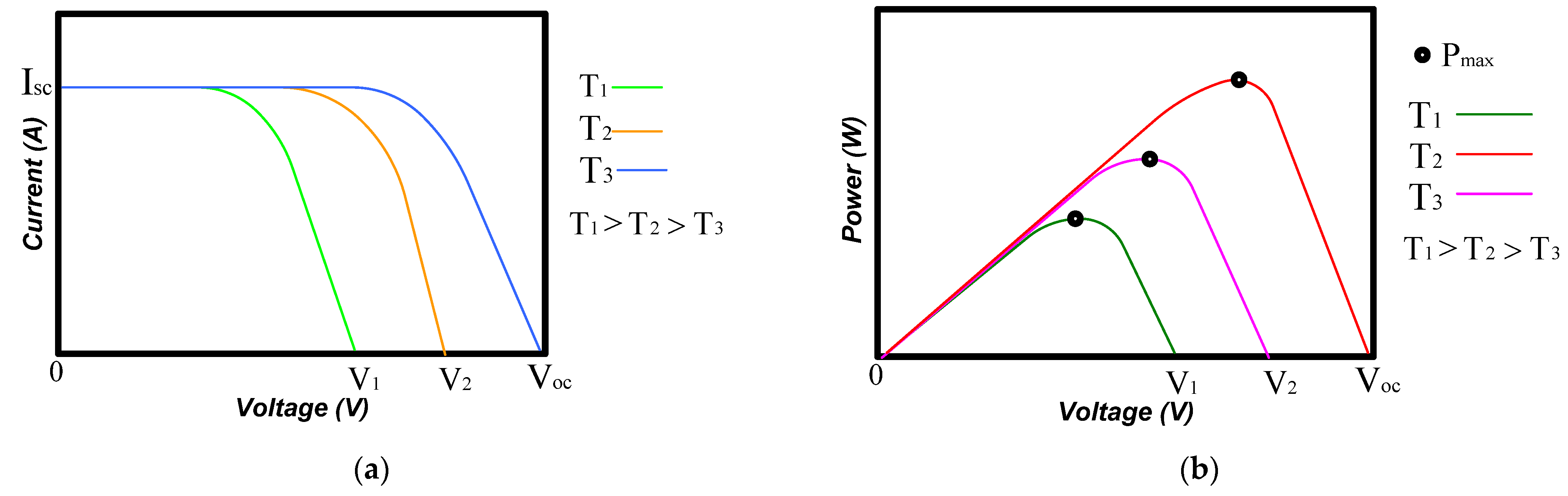
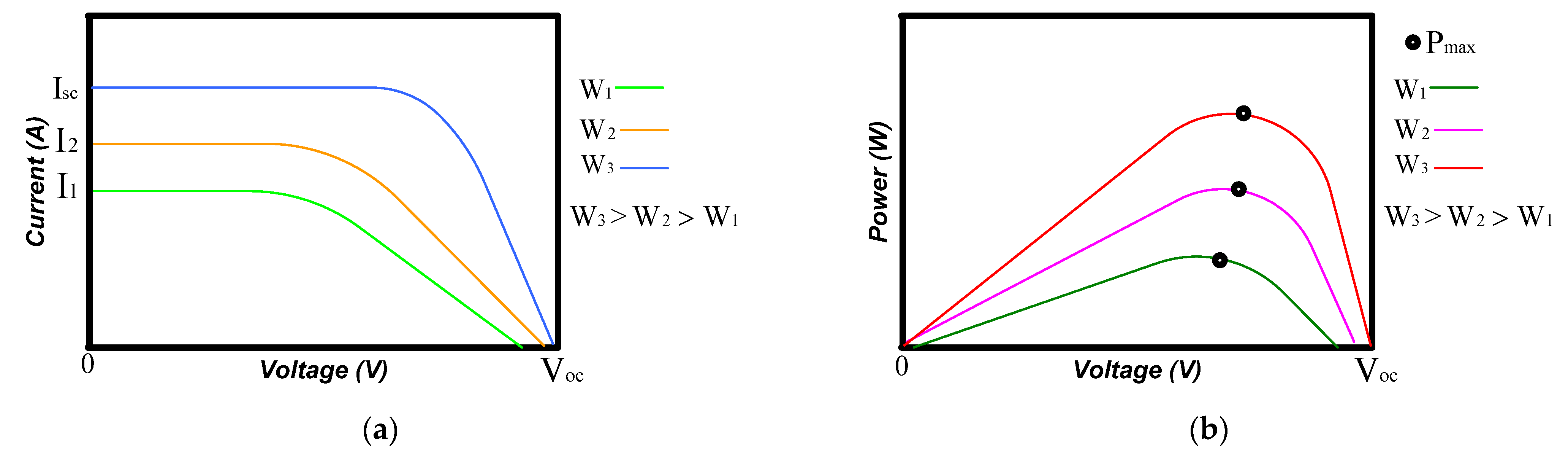
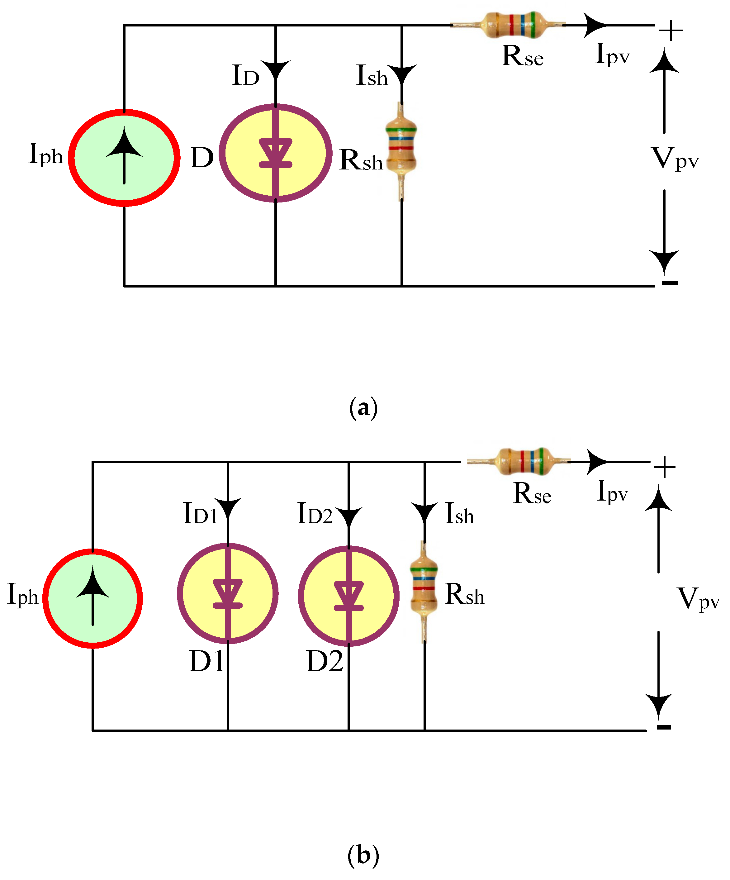
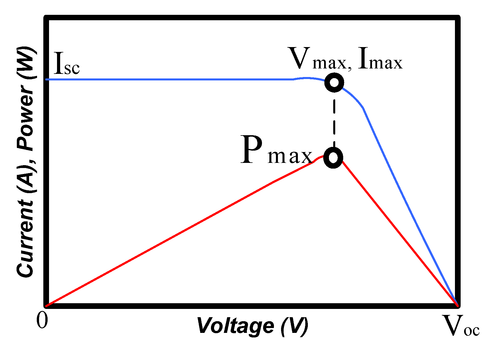
2. Modeling of PV Cell


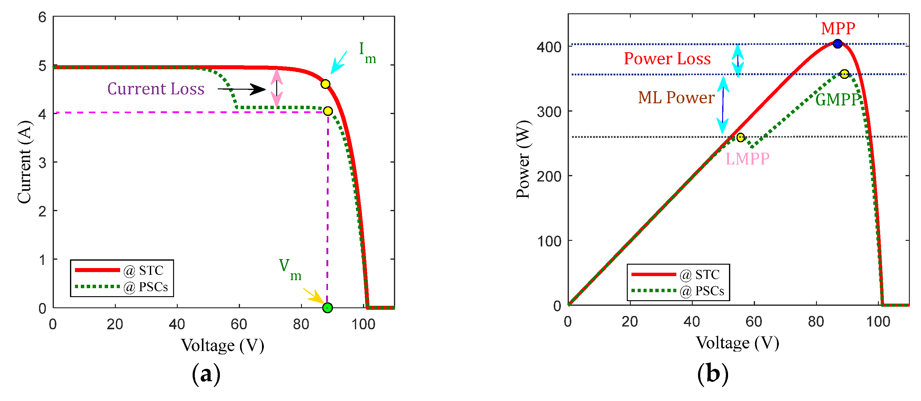
3. Partial shading Effect
- Non-linear PV module (I–V) characteristic curve with multiple LMPP. As a result, shading causes hot spots and damages the solar cells;
- Current and voltage mismatch in PV array;
- Many peaks in the (P–V) characteristic curve with an increase in shading conditions.
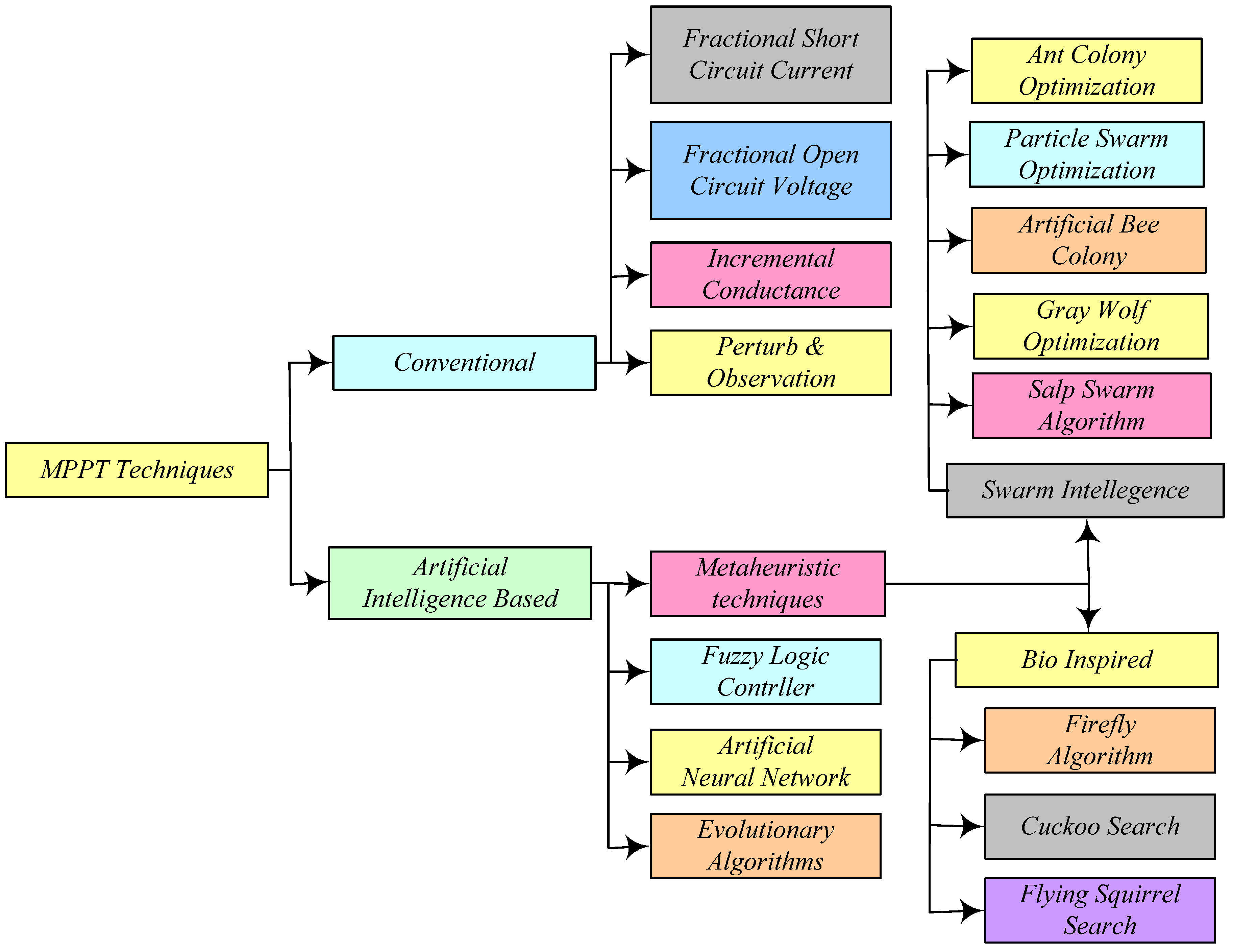
4. MPPT Algorithms
4.1. Conventional MPPT Techniques
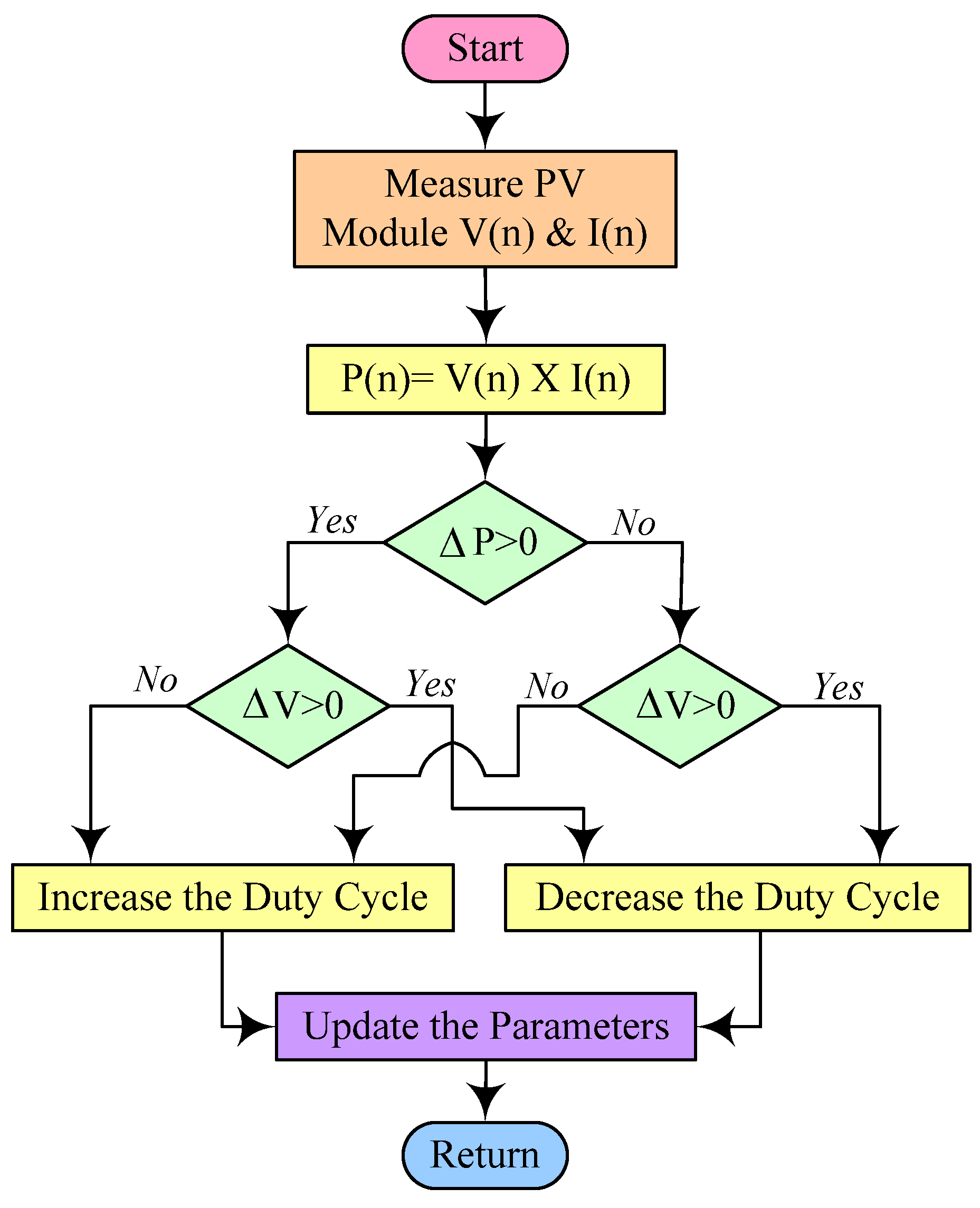
4.1.1. Perturb and Observe
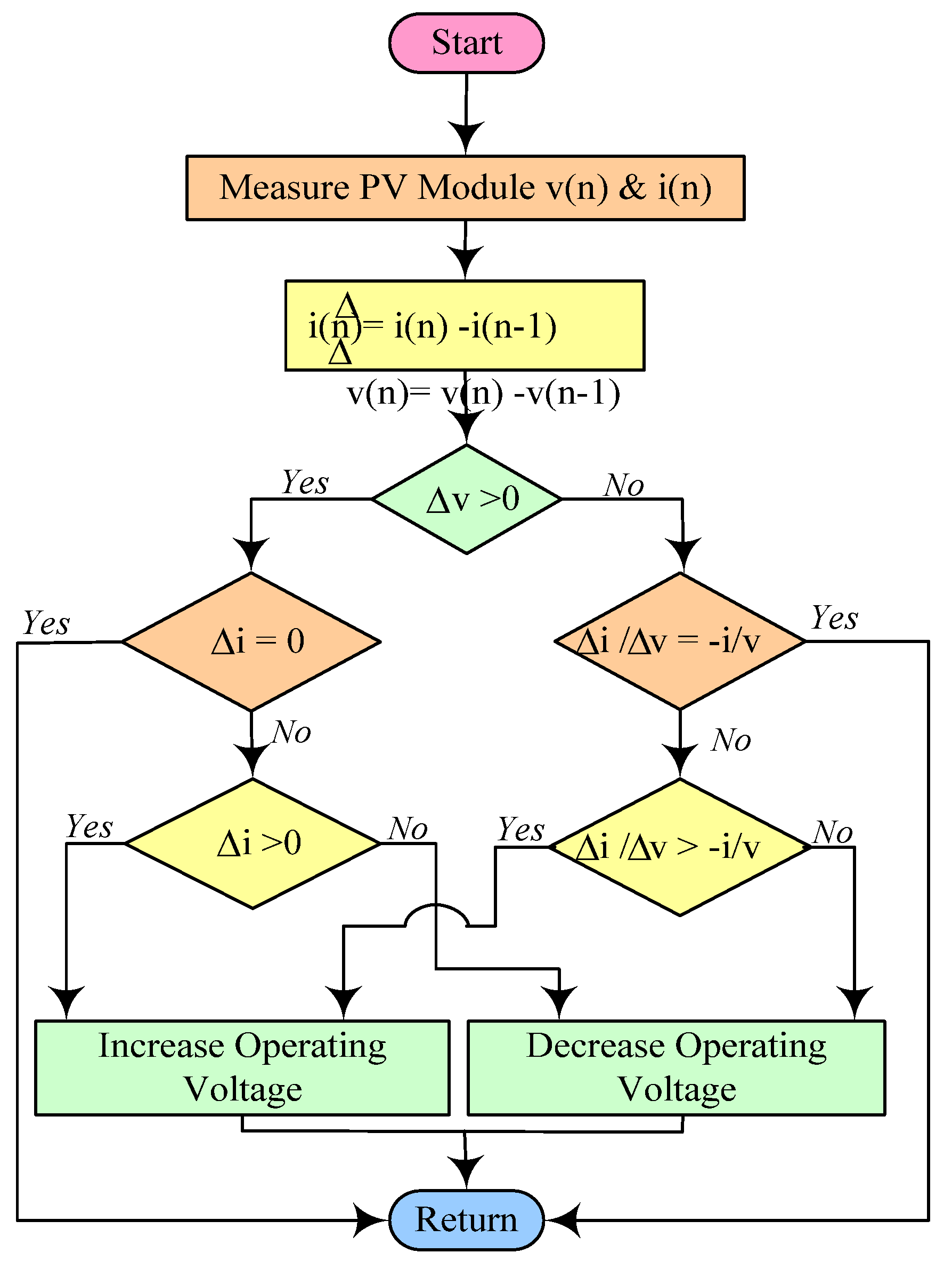
4.1.2. Incremental Conductance
| If | At MPP | |
| If | At the right side of MPP | |
| If | At the left side of MPP |
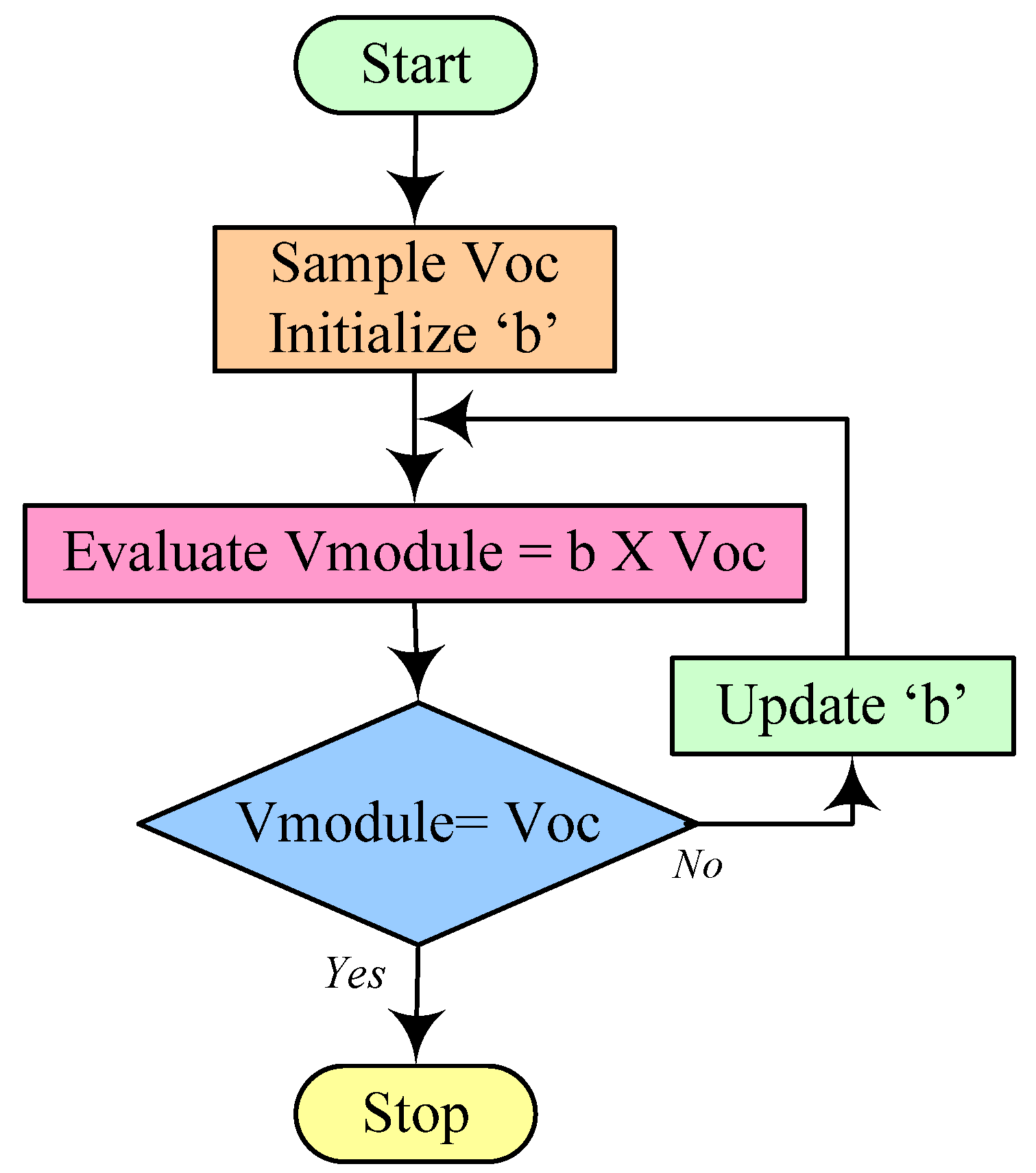
4.1.3. Fractional Open-Circuit Voltage Technique
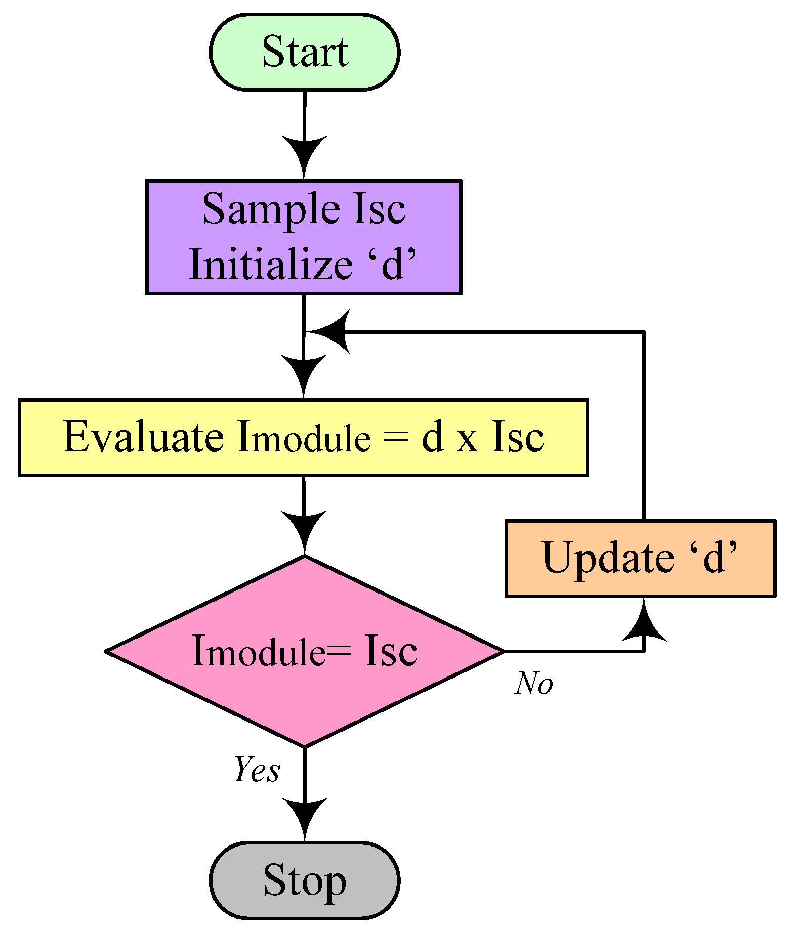
4.1.4. Fractional Short-Circuit Current Technique
4.2. Swarm Intelligence MPPT Techniques
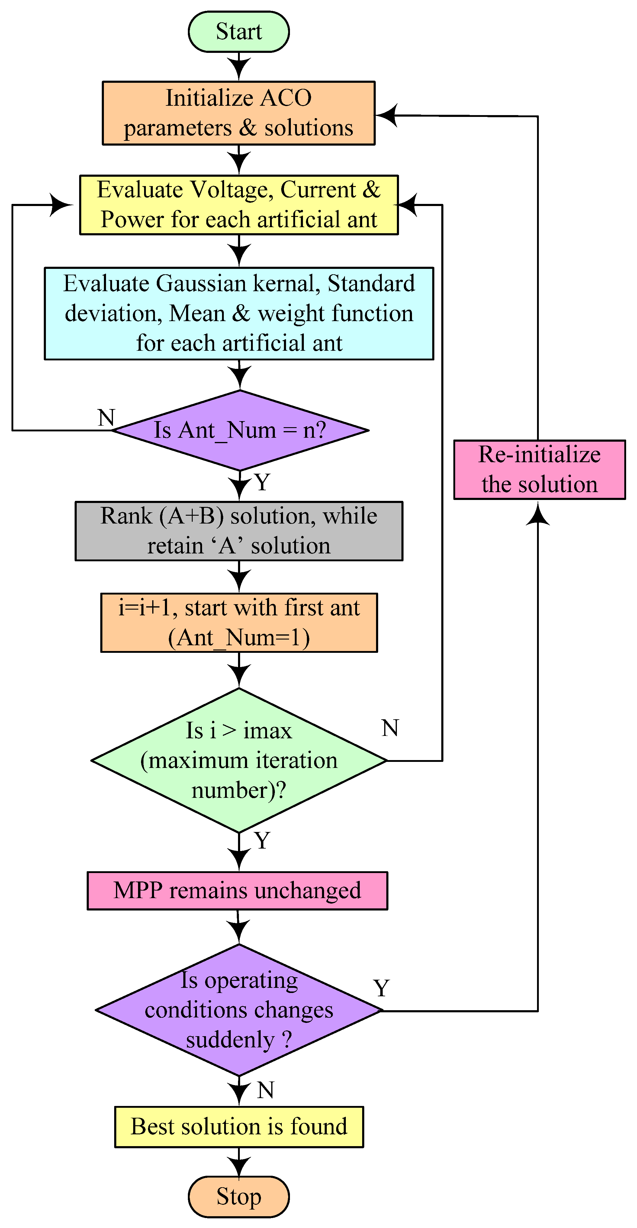
4.2.1. Ant colony Optimization
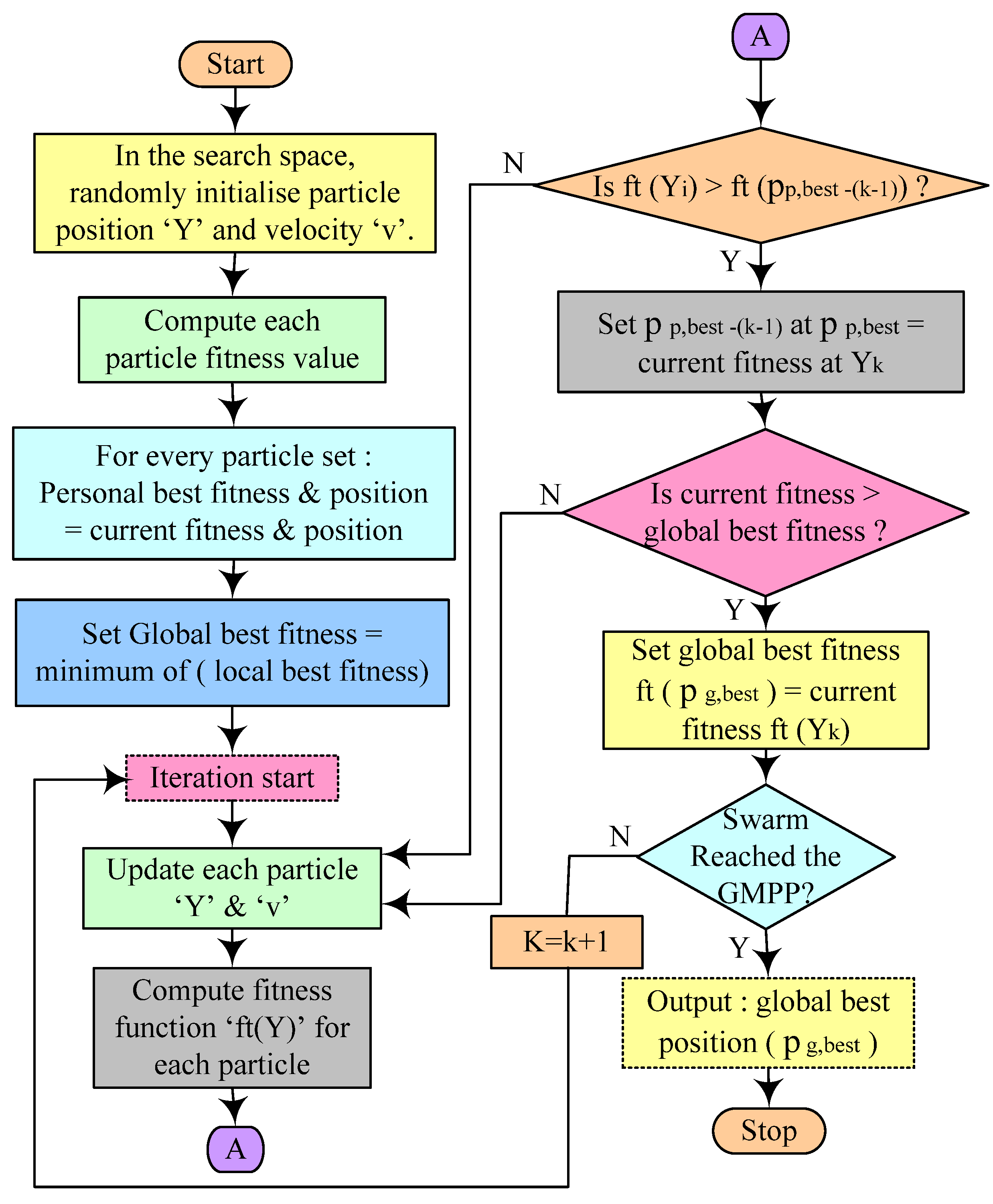
4.2.2. Particle Swarm Optimization
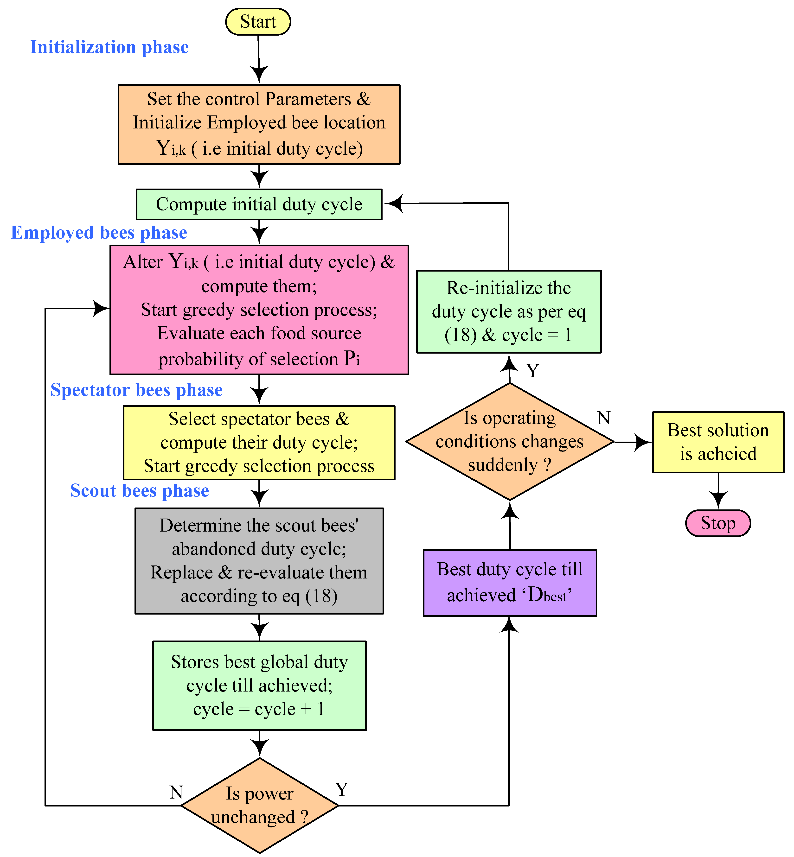
4.2.3. Artificial Bee Colony
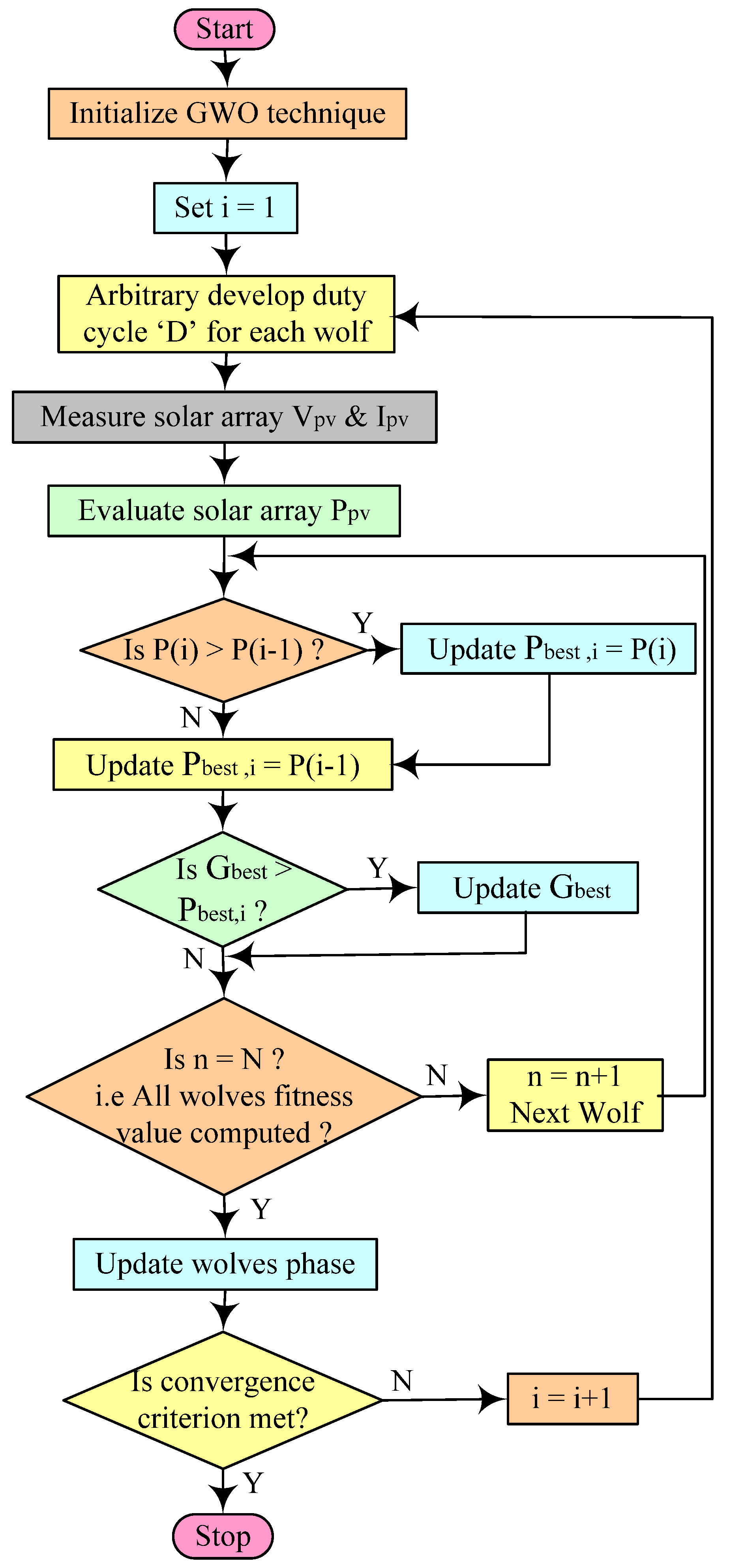
4.2.4. Grey Wolf Optimization
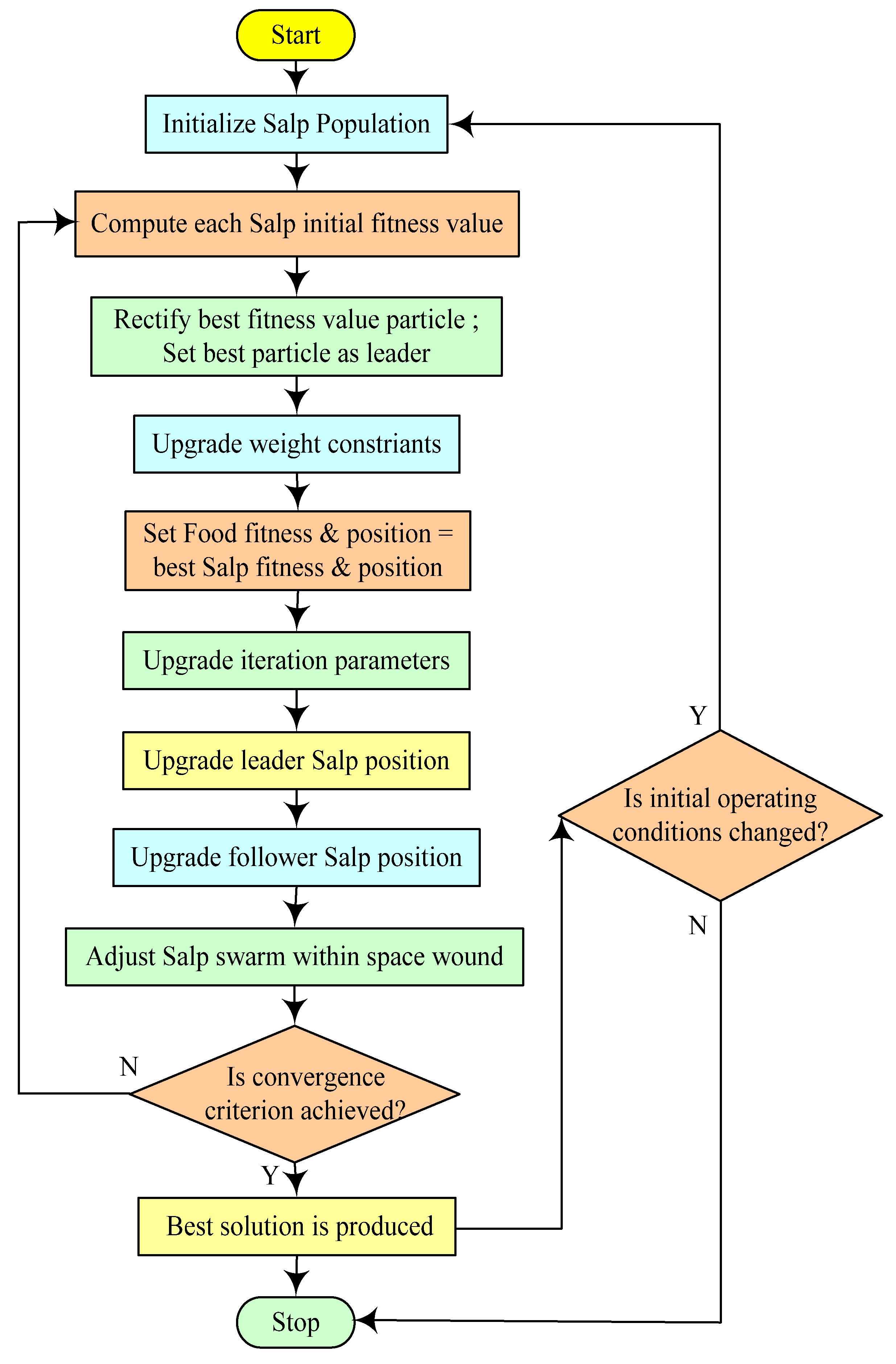
4.2.5. Salp Swarm Algorithm (SSA)


| Authors [Reference No.] | Optimization Techniques | Best Optimization Techniques | PV Module Pm (W) | PV System Size | GMPP (W) | Improved GMPP (%) | Irradiance (W/m2) | Shading Patterns | Tracking Time (s) |
|---|---|---|---|---|---|---|---|---|---|
| Krishnan SG et al. [54] | Proposed, ACO, PSO, P&O | Proposed ACO | 20 | 4 × 4 3 × 6 | 63, 48.75 | 1.00, 32.29 | NA | Non uniform | 1.5, 1.56 |
| Sridhar R et al. [55] | ACO, P&O | ACO | NA | 3 PV module in series | 61.4 | 261.1 | NA | Non uniform | 0.076 |
| Alshareef M et al. [56] | APSO, PSO, P&O | APSO | NA | NA | 40.56, 73.33, 76.51 | 13.07, 4.29, 73.49 | NA | NA | 1.9–2.4 |
| Panda KP et al. [57] | Modified PSO PSO, P&O | Modified PSO | 60 | 4 × 1 | 116.4 | 105.3 | 1000–400 | Non uniform | 0.9 |
| Gopalakrishnan SG et al. [58] | Proposed PSO PSO, P&O | Proposed PSO | 20 | 4 × 4 3 × 6 | 56.25, 48.75 | 18.42, 32.29 | NA | Non uniform | 1.9, 1.7 |
| Mao M et al. [59] | Proposed, PSO | Proposed | 83.2824 | 3 × 1 | 245.31, 60.8, 148.38 | −0.28, 32.83, 1.54 | 1000–300 | Non uniform | 0.012–0.016 |
| Koad RBA et al. [60] | LIPSO, P&O INC, PSO | LIPSO | NA | 4 × 1 | 60.64, 48.76, 36.58, 24.29, 11.67 | 4.98, 12.79, 8.80, 16.23 | 1000–200 | Uniform | NA |
| Belghith OB et al. [61] | PSO Fuzzy_TS P&O | PSO | 150 | 1 PV module | 148.46, 122.81, 55.67 | 1.48, 2.36, 5.69 | 1000–400 | Non uniform | 0.003–0.043 |
| Obukhov S et al. [62] | VCPSO, CFPSO | VCPSO | 320.4 | 3 PV module in series, 4 PV module in series, 8 PV module in series | 960.2, 478.8, 477.8, 312.3 | 0.376, 0.041, 0.378, 0.192 | 1000–100 | Non uniform | 0.48–0.66 |
| Li H et al. [63] | OD-PSO Firefly, P&O-PSO | OD-PSO | 101.3 | 3 PV module in series | 112.85, 110.85 | −10.48, 4.00 | 1000–300 | Non uniform | 1.64, 2.08 |
| Suhardi D et al. [64] | GWO INC | GWO | 200 | NA | 203.2, 142.2, 35.9 | 112.19, 54.76, −50.72 | 1000–400 | Non uniform | 0.55 |
| Kumar CS [65] | EGWO GWO PSO | EGWO | 200 | 4 PV module in series, 2 × 2 | 522.629, 401.044, 522.763, 401.027 | 0.938, 2.707, −0.05, 7.91 | 1000–400 | Non uniform | 3.6–4.8 |
| Shi JY et al. [66] | P&O, PSO GWO, GWO-P&O GWO-GSO | GWO-GSO | 60 | 4 × 1 | 100.72 | 100.95 | 1000–300 | Non uniform | 0.64 |
| Ilyas M [67] | Modified GWO GWO | Modified GWO | 100 | 4 PV module in series, 2 × 2 | 444.65, 435.76 | 0.234, 0.045 | NA | Non uniform | 0.189, 0.21 |
| Kraiem H et al. [68] | PSO, GWO | PSO | 249 | 4 PV module in series | 645.6, 633.9, 359.1 | 0.077, 0.939, 0.447 | 1000–200 | Non uniform | 0.0561–0.071 |
| Jamaludin MNI et al. [69] | SSA PSO GOA GWO BOA HC | SSA | 59.85 | 4 × 1 | 136.3, 114.3, 176.9 | 23.5, 107.7, 58.93 | 1000–500 | Non uniform | 0.22, 2.3, 4.2 |
| Dagal I et al. [70] | Hybrid SSPSO P&O FA DE ISSA | SSPSO | 60 | 4 PV module in series | 124.09 | 6.55 | 1000–400 | Non uniform | 0.29 |
| Krishnan S et al. [71] | SSO WOA GWO | SSO | 220.5 | 3 PV module in series 2X2 | 294.8, 41.8, 525.4, 38.5, 445.2, 02.7 | 5.58, 10.04, 39.92, 14.67, 14.97, 28.43 | 750–500 | Non uniform | 0.0245–0.0749 |
| Farzaneh J et al. [72] | P&O, FFA, PSO, DE, SSA, ISSA | ISSA | 60 | 4 PV module in series | 115.59 | 6.53 | 1000–400 | Non uniform | 1.22 |
| Ali MHM [73] | P&O, SSO | SSO | NA | NA | 843.5 | 2.55 | 200 | Uniform | 0.72 |
| Balaji V et al. [74] | Hybrid SSPO SS, PO | Hybrid SSPO | 50 | 4 PV module in series | 50.3, 85.1, 78.2, 96.1 | 27.66, 0.09, 24.32, 51.10 | 1000–200 | Non uniform | 0.52–0.57 |
| Restrepo C et al. [75] | ABC-P&O GMPPT P&O | ABC-P&O | 200.143 | 4 PV module in series | 597.95 | 54.19 | 900–120 | Non uniform | NA |
| Sawant PT et al. [76] | ABC, PSO | ABC | 75 | NA | 74, 61 | 2.77, 3.38 | 1000–800 | Non uniform | NA |
| Li N et al. [77] | P&O, PSO ABC, MABC | Modified MABC | NA | 2 PV module in series | 850 | 70.68 | 1000–800 | Non uniform | 0.39 |
| Wan Y et al. [78] | SSA-GWO, P&O, PSO, SSA | SSA-GWO | 35 | 3 PV module in series | 104.88, 44.55, 69.32 | 0.788, 28.60, 1.612 | 1000–300 | Non uniform | 0.46, 0.53, 0.47 |
| Hayder W et al. [79] | IPSO, PSO-P&O, ANN-PSO | IPSO | 120 | NA | 119.9720, 69.9888, 94.9073, 45.3924 | NA | 1000–400 | Non uniform | 1.5 |
| Almutairi A et al. [80] | OGWO, P&O | OGWO | 60 | NA | 60, 47.8, 23 | 32.77 | NA | Non uniform | 0.5, <1, |
| Sharma A et al. [81] | TSA-PSO, FPA, GWO, TSA, PSO, P&O | TSA-PSO | 85 | 3 PV module in series | 103.36, 122.88, 156.84 | 22.20, 5.97, 13.11 | 1000–300 | Non uniform | 0.38, 0.54, 0.40 |
| Chao K-H et al. [82] | I-ABC, PSO, P&O, ABC | I-ABC | 20 | 4 × 3 | 246.6, 198.6, 148.8, 107.1, 77.1 | 0.08, 2.00, 0.881, 17.43, 66.88 | NA | Non uniform | 0.38, 0.63, 0.89, 1.48, 1.14 |
| Alaraj M et al. [83] | HGWO, PSO, INC | HGWO | 450 | 5 × 5 | 8256, 6441, 6347, 5567 | 13.23, 13.09, 20.50, 22.86 | 1000–400 | Non uniform | 0.08, 0.07 |
| Windarko N A et al. [84] | Proposed, DE, FF, PSO, GWO | Proposed | 100 | 3 PV module in series | 172.9, 170.9, 80.9 | 5.81, 65.60, 226.2 | 1000–100 | Non uniform | 0.45, 0.41, 0.52 |
| Chawda G S et al. [85] | ICPSO, P&O, INC, GA-based FLC, PSO-based FLC PSO-GA-FLC | ICPSO | NA | NA | 97.3, 60, 94.2 | 7.955, 11.77 | 1000–300 | Non uniform | 0.1 |
| Authors [Reference No.] | Pros | Cons |
|---|---|---|
| Krishnan SG et al. [54] |
|
|
| Sridhar R et al. [55] |
|
|
| Alshareef M et al. [56] |
|
|
| Pandal KP et al. [57] |
|
|
| Gopalakrishnan SK et al. [58] |
|
|
| Mao M et al. [59] |
|
|
| Koad RBA et al. [60] |
|
|
| Belghith OB et al. [61] |
|
|
| Obukhov S et al. [62] |
|
|
| Li H et al. [63] |
|
|
| Suhardi D et al. [64] |
|
|
| Kumar CS et al. [65] |
|
|
| Shi JY et al. [66] |
|
|
| Ilyas M et al. [67] |
|
|
| Kraiem H et al. [68] |
|
|
| Jamaludin MNI et al. [69] |
|
|
| Dagal I et al. [70] |
|
|
| Krishnan S et al. [71] |
|
|
| Farzaneh J et al. [72] |
|
|
| Ali MHM [73] |
|
|
| Balaji V et al. [74] |
|
|
| Restrepo C et al. [75] |
|
|
| Sawant PT et al. [76] |
|
|
| Li N et al. [77] |
|
|
| Wan Y et al. [78] |
|
|
| Hayder W et al. [79] |
|
|
| Almutairi A et al. [80] |
|
|
| Sharma A et al. [81] |
|
|
| Chao K-H et al. [82] |
|
|
| Alaraj M et al. [83] |
|
|
| Windarko N A et al. [84] |
|
|
| Chawda G S et al. [85] |
|
|
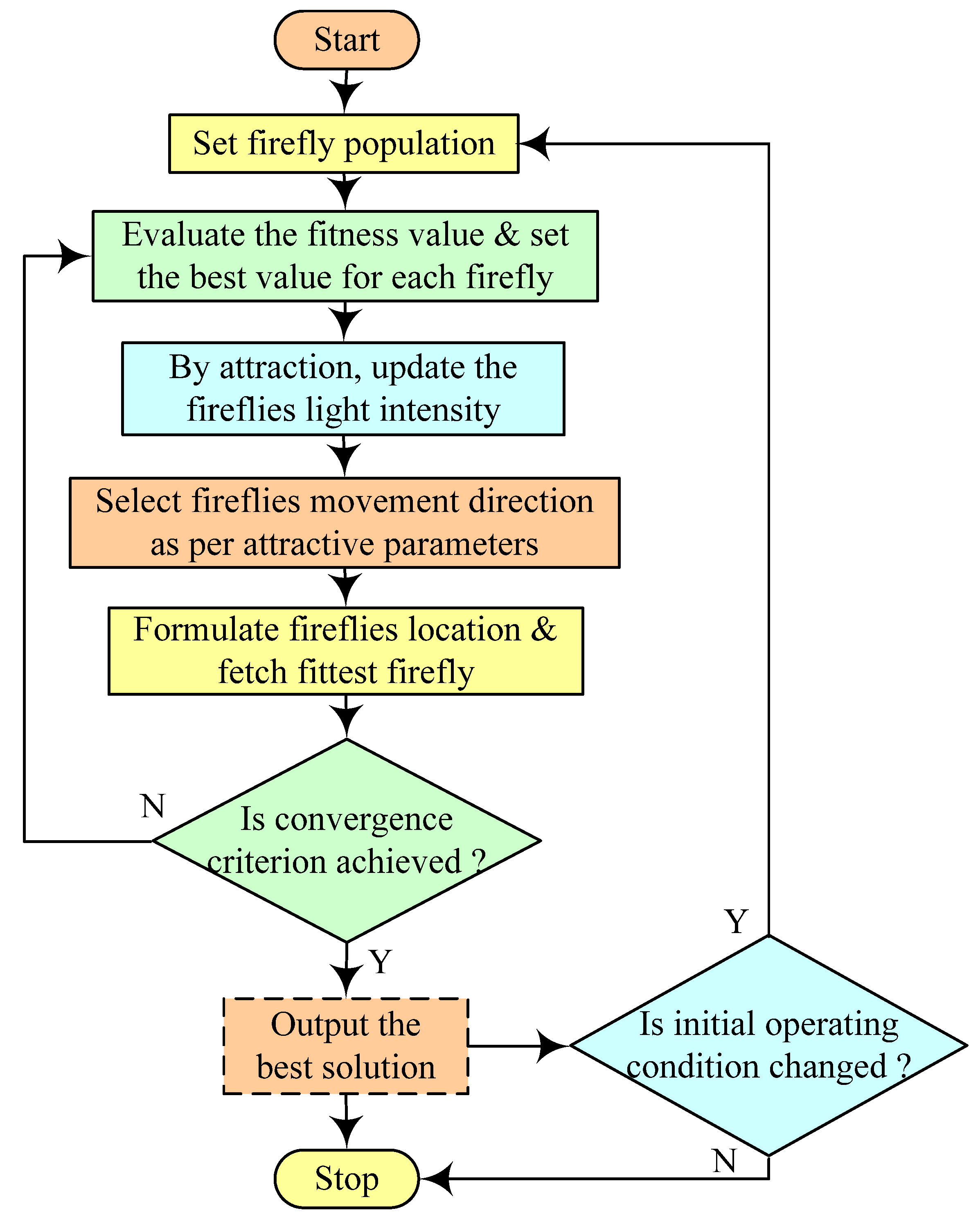
4.3. Bio Inspired Techniques
4.3.1. Firefly MPPT Algorithm
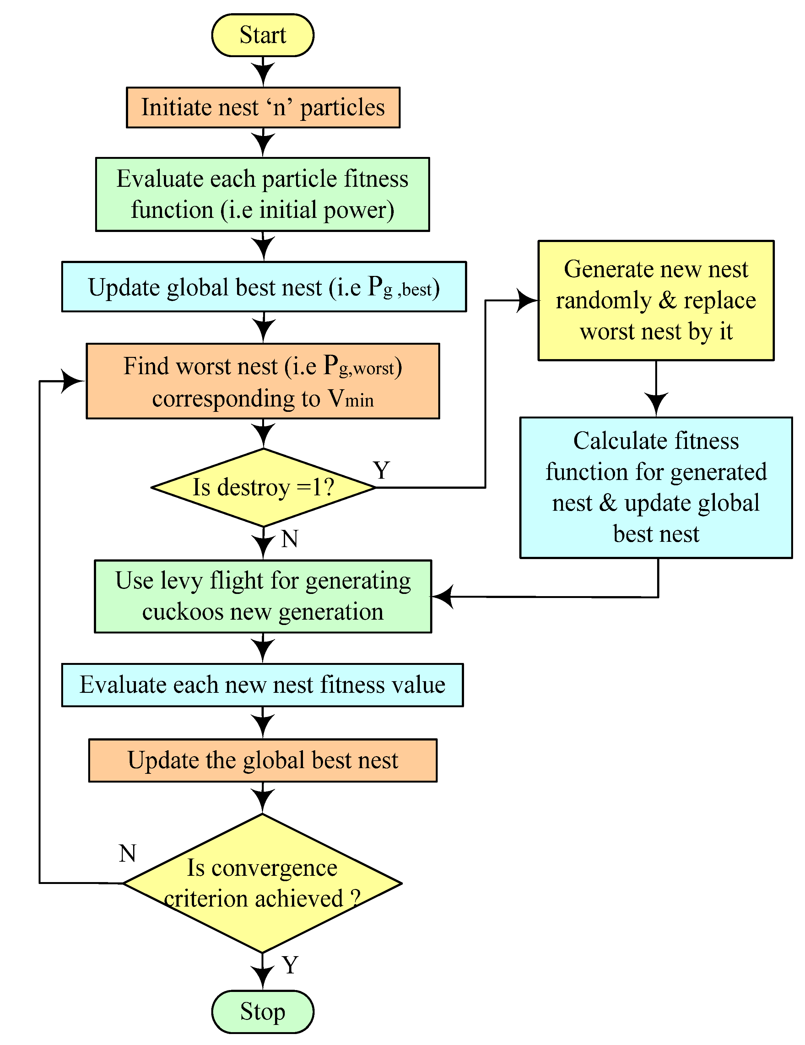
4.3.2. Cuckoo Search
- Every cuckoo bird merely lays one egg at a time in a hastily chosen host nest;
- The cuckoos’ subsequent generation will be carried on by the superior eggs’ nest (i.e., the best solutions);
- In the hunt area, the entire number of reachable host nests is fixed.
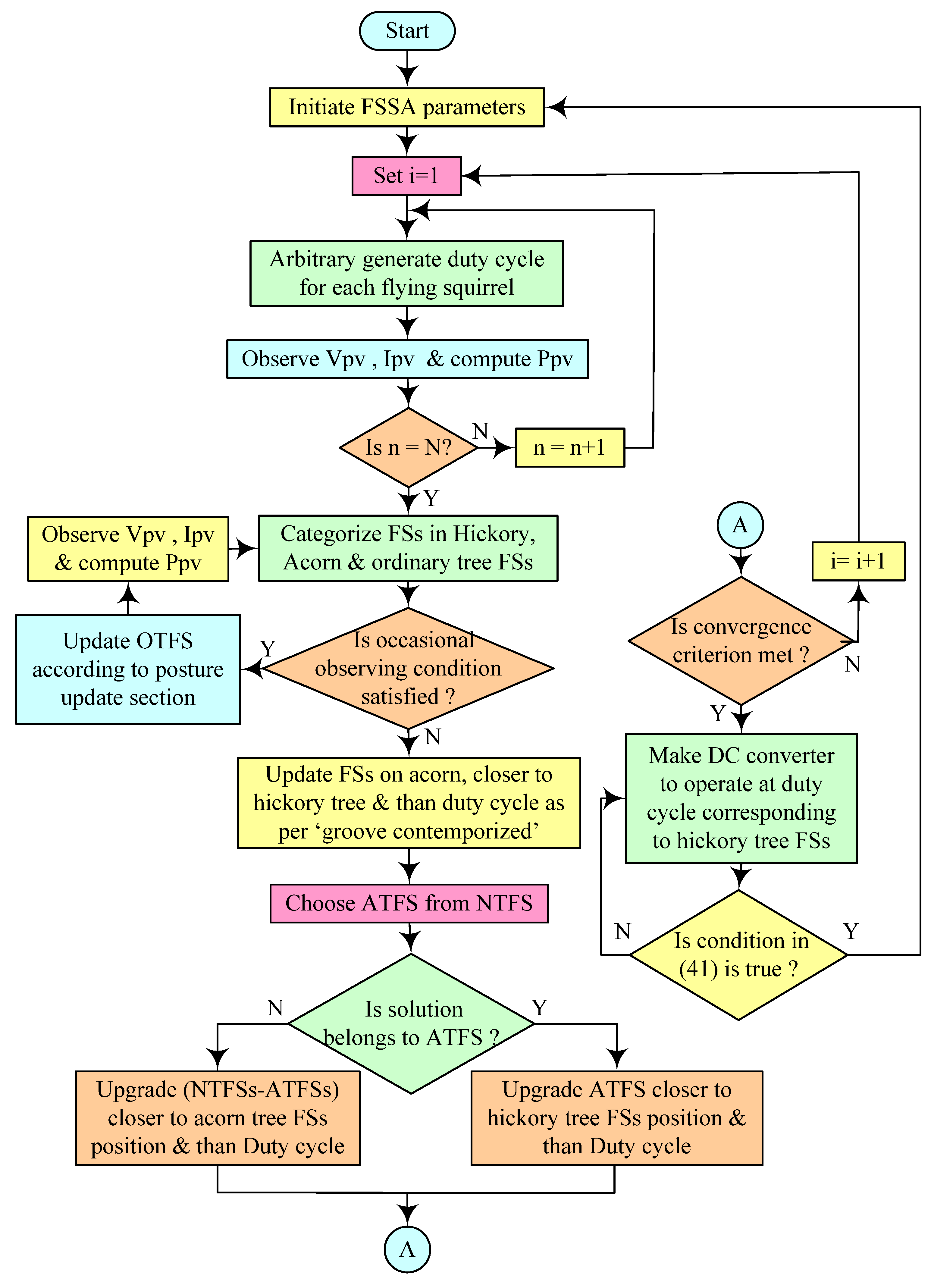
4.3.3. Flying Squirrel Search Optimization
- BS (hickory nut tree);
- CBS (acorn nut tree);
- US (ordinary tree).
- Declaration and categorization: The duty cycle at which the system yields maximum power is considered as hickory tree, while acorn trees are considered as the most excellent FS positions;
- Posture update: After the examination of occasional observing situation, the duty cycle is updated, and wellness is assessed from that point.
- Groove contemporized: Squirrels of hickory tree maintain their position. The squirrels on acorn tree, on the other hand, find a way to access the hickory tree. The arbitrarily chosen squirrel (ATFS) from normal trees chooses the hickory tree, while the leftover (NTFS-ATFS) is pressed to the acorn tree. The duty cycle is changed:
- Convergence Resolution: If the utmost number of iterations has been reached, the algorithm is terminated and gives the duty cycle at the point where the converter follows GMPP.
- Re-initialization: In rapidly changing environmental conditions, the duty ratio (FSs posture) is reinitialized to hunt new GMPP in accordance with Equation (41).
| Authors [Reference No.] | Optimization Techniques | Best Optimization Techniques | PV Module Pm (W) | PV System Size | GMPP (W) | Improved GMPP (%) | Irradiance (W/m2) | Shading Patterns | Tracking Time (s) |
|---|---|---|---|---|---|---|---|---|---|
| Saad W et al. [90] | Proposed FA, P&O | Proposed | 200 | 1PV module | 201.7 37.7 | 2.40, 8.02 | 1000 and 200 | Non uniform | NA |
| Farzaneh J et al. [91] | MFA, P&O PSO, FA | MFA | 200.143 | 4 PV module in series | 397.52 | 9.41 | 1000–400 | Non uniform | 2.22 |
| Nusaif AI et al. [92] | MFA, P&O PSO, FA | MFA | 265.737 | 3 × 3 | 1264, 1206, 1582, 834 | 1.77, 31.08, 17.70, 27.91 | 1000–100 | Non uniform | 0.085–0.124 |
| Abo-Khalil AG et al. [93] | OFA, FA P&O | OFA | NA | NA | 48, 36.5, 29 | 0.418, 2.24, 34.88 | NA | Non uniform | 0.2–0.33 |
| Shi J-Y [94] | INC-FA, P&O INC, FA | INC-FA | 60 | 4 × 1 | 81.4 | 76.19 | 1000–100 | Non uniform | 0.98 |
| Omar FA et al. [95] | Proposed FA P&O | Proposed FA | NA | 3 PV module in series | 100,150,200, 300,400,500 | 25.00, 2.04, 108.33, 100, 110.52, 170.27 | NA | Non uniform | 1.3 |
| Chitra A et al. [96] | INC, FA, MFA | MFA | 200.143 | 2 PV module in series | 330, 255 | 6.24, 3.23 | 1000–600 | Non uniform | 0.0018–0.0064 |
| Mosaad MI et al. [97] | CS, NN, INC | CS | 59.9 | 1PV module | 60.47, 48.24 | 2.68, 3.36 | 1000–800 | uniform | NA |
| Shi J-Y et al. [98] | ICS, CS PSO, P&O | ICS | 60 | 4 PV module in series | 87.547 | 74.97 | 1000–200 | Non uniform | 0.88 |
| Hidayat T et al. [99] | CSA, P&O | CSA | 72 | 2 PV module in series | 97, 107.92, 107.63, 114.94, 124.56, 74.53, 72.58 | 45.86, 70.75, 63.99, 77.89, 81.52, 5.40, 0.276 | 944–495 | Non uniform | NA |
| Bilgin N et al. [100] | FFO, PSO, CSO, BOA | FFO | NA | 3 PV module in series | 531.46, 377.63 | 5.73, 4.26 | 1000–278 | Non uniform | NA |
| Ibrahim A-W et al. [101] | CSA, MPSO, MP&O, ANN | CSA | 250 | 4 PV module in series | 699.6, 928.5, 534.7, 694.7 | 67.93, 29.40, 13.25, 4.215 | 1000–400 | Non uniform | 0.5–0.7 |
| Bentata K et al. [102] | DCSA, CSA | DCSA | 249 | 2 × 2, 4 PV module in series, 3 × 2, 6 PV module in series | 989.29, 482.06, 797.3, 656.45 | 0.00, 13.31, 6.40, 16.09 | 1000–200 | Non uniform | 0.046- 0.085 |
| Singh N et al. [103] | FSSO, P&O, PSO, GWO | FSSO | 40 | 4 PV module in series, 2 × 2 | 61.66, 48.65, 79.75, 35.37 | 107.53, 85.68, 61.73, 3.23 | 900–100 | Non uniform | 0.3–1.8 |
| Fares D et al. [104] | ISSA, SSA, PSO, GA | ISSA | 135 | 3 PV module in series | 227.83, 142.82, 98.79 | 0.065, 0.098, 0.050 | 900–100 | Non uniform | 0.2 |
| Al-Shammaa A A et al. [105] | CS, PSO | CS | NA | 4 PV module in series | 293.57, 415.38, 578.96 | 0.00, 0.67, 0.52 | 1000–200 | Non uniform | 1.32, 1.29, 1.28 |
| Watanabe R B et al. [106] | FF, P&O | FF | 213.15 | 3 PV module in series | 638.7, 553.1, 316.9 | 0.251, 31.87, 58.05 | 1000–300 | Non uniform | 0.18, 0.22, 0.21 |
| Authors [Reference No.] | Pros | Cons |
|---|---|---|
| Saad W et al. [90] |
|
|
| Farzaneh J et al. [91] |
|
|
| Nusaif AI et al. [92] |
|
|
| Abo-Khalil AG et al. [93] |
|
|
| Shi JY [94] |
|
|
| Omar FA et al. [95] |
|
|
| Chitra A et al. [96] |
|
|
| Mosaad MI et al. [97] |
|
|
| Shi J-Y et al. [98] |
|
|
| Hidayat T et al. [99] |
|
|
| Bilgin N et al. [100] |
|
|
| Ibrahim A-W et al. [101] |
|
|
| Bentata K et al. [102] |
|
|
| Singh N et al. [103] |
|
|
| Fares D et al. [104] |
|
|
| Al-Shammaa A A et al. [105] |
|
|
| Watanabe R B et al. [106] |
|
|
4.4. Other AI-Based MPPT
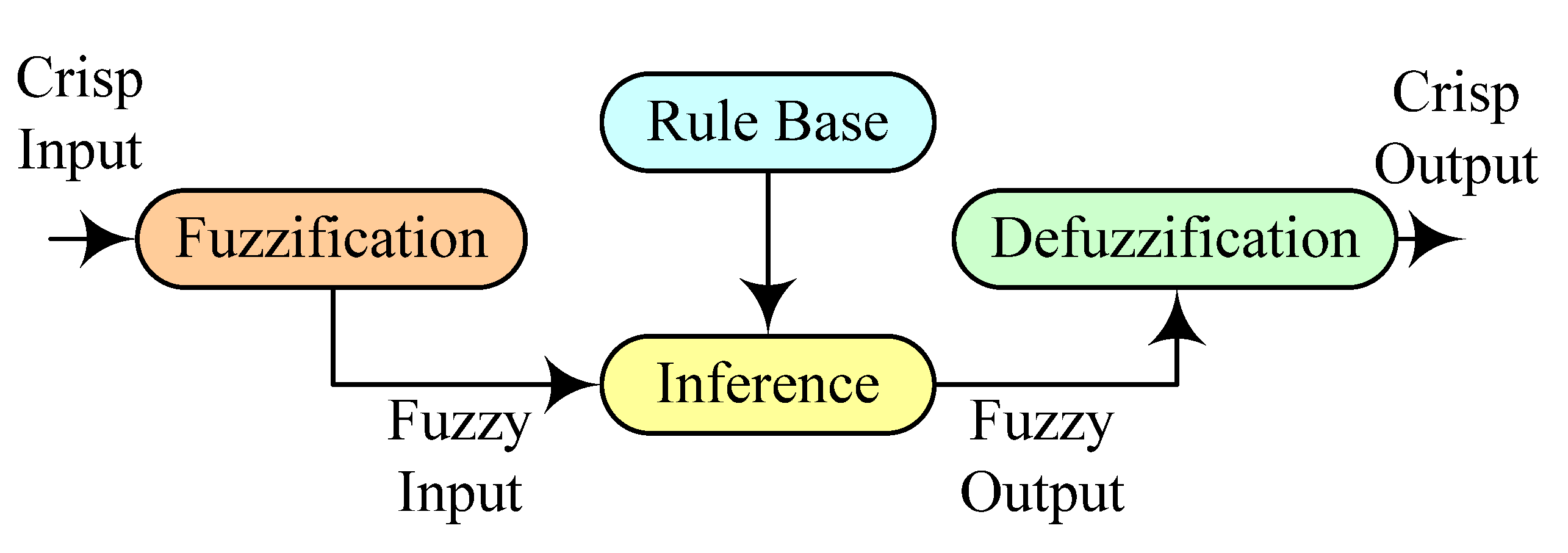
4.4.1. Fuzzy Logic Control
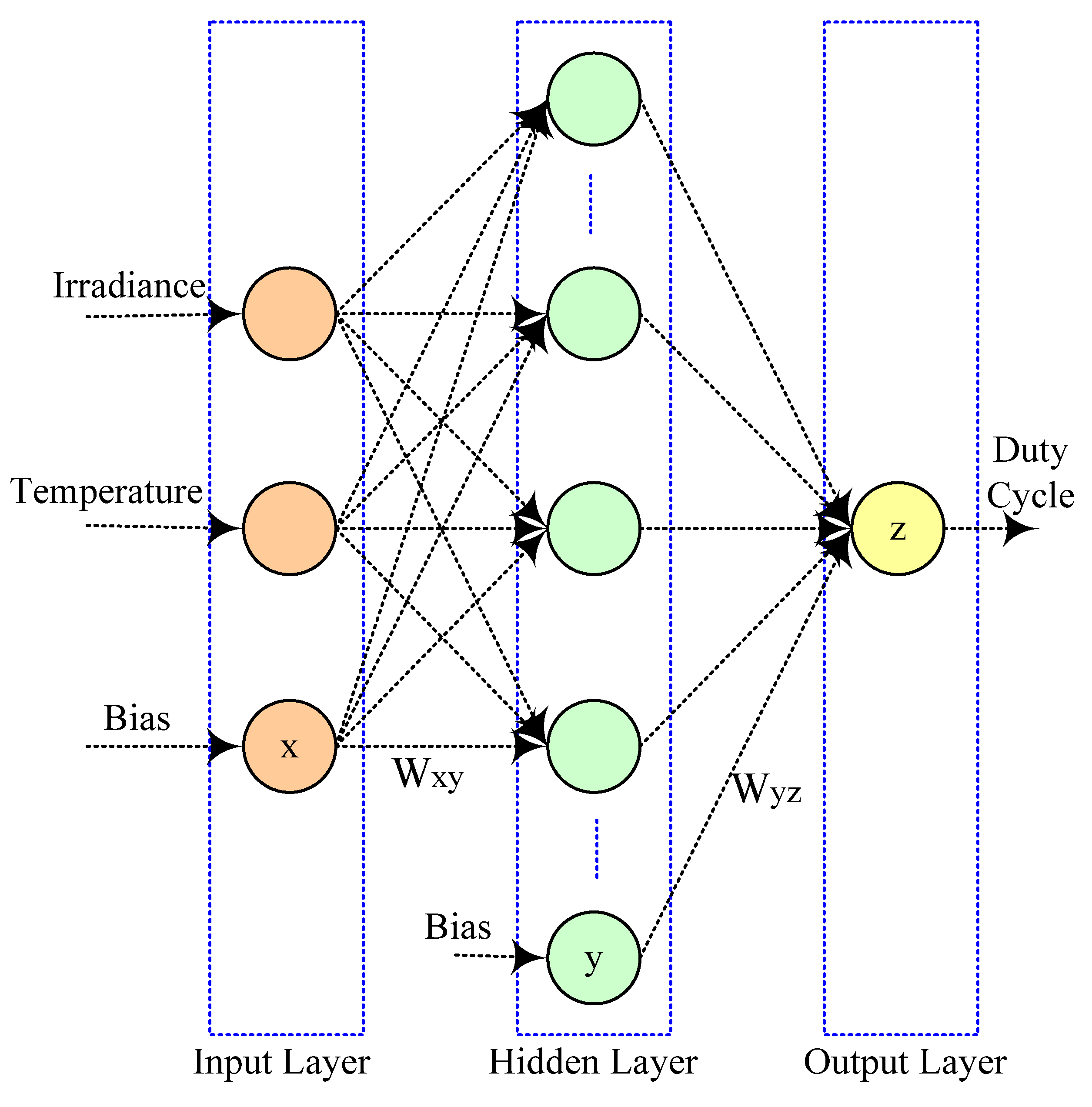
4.4.2. Artificial Neural Network
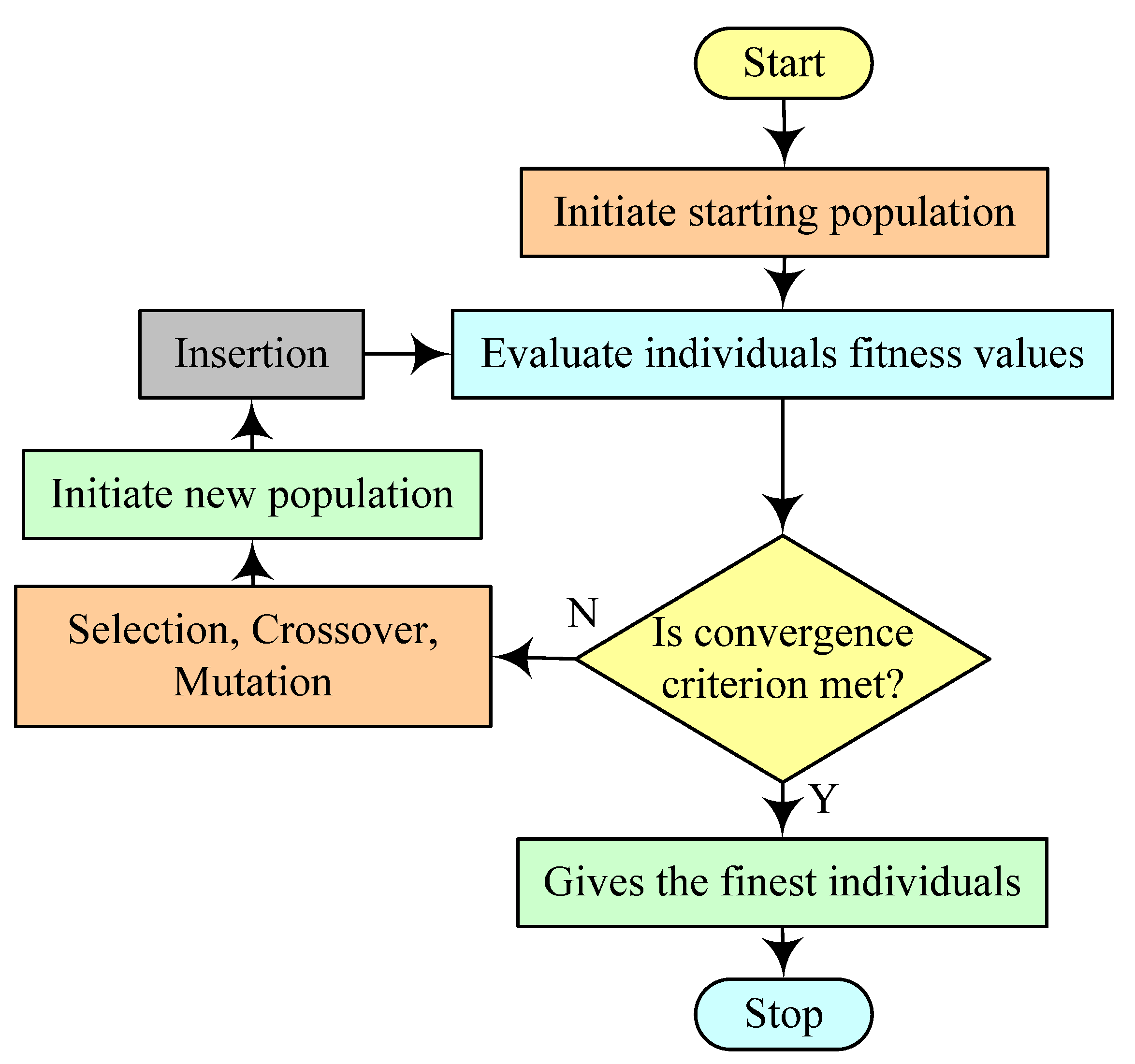
4.4.3. Evolutionary Computational Techniques
| Authors [Reference No.] | Optimization Techniques | Best Optimization Techniques | PV Module Pm (W) | PV System Size | GMPP (W) | Improved GMPP (%) | Irradiance (W/m2) | Shading Patterns | Tracking Time (s) |
|---|---|---|---|---|---|---|---|---|---|
| Verma P et al. [111] | AFLC, FLC P&O | AFLC | 360 | 3 PV module in series | 521.5, 250.6, 198.1 | 7.30, 0.642, 4.26 | 900–100 | Non uniform | 0.1–0.19 |
| Rahman MM et al. [112] | PSO-ANN PSO | PSO-ANN | 60.53 | 4 PV module in series | 135.9, 202.1 | 0.00, −0.04 | 900–400 | Non uniform | 0.22, 0.21 |
| Farzaneh J [113] | Proposed P&O, PSO | Proposed | 60 | 3 PV module in series | 87.12, 116.74 | 46.00, 94.17 | 1000–300 | Non uniform | 0.15, 0.1 |
| Manikandan PV [114] | Proposed P&O | Proposed | 320 | 1 PV module | 36.88, 37.2, 37.66 | 53.73, 50.12, 51.36 | 1200–400 | Non uniform | NA |
| Al-Majidi SDet al. [115] | ANFIS FLC, P&O | ANFIS | 185 | 5 PV module in series | 924 | 0.2168 | 1000 | Uniform | 0.07 |
| Aymen J et al. [116] | Neuro fuzzy Fuzzy | Neuro fuzzy | 60 | 1PV module | 50.262, 45.736, 40.856, 35.633, 30.156 | 0.001, −0.004, 0.0171, 0.0533, 0.0763 | 1000–600 | Non uniform | NA |
| Farajdadian S [117] | AF-FA AF-PSO SF, PSO, P&O | AF-FA | 220.7 | NA | 220.5, 175.1, 124.3 | 1.37, 20.26, 72.87 | 1000–600 | Non uniform | NA |
| Eltamalya AM et al. [118] | GWO-FLC PSO | GWO-FLC | 185.22 | NA | 54.6, 92.8 | 40.00, 20.51 | 1000–200 | Non uniform | NA |
| Chen Y-T et al. [119] | Proposed fixed-step INC FLC-HC ASVSS | Proposed | 60 | NA | 157.3,46.83 | 5.92, 2.51 | 1000 and 300 | Non uniform | 0.42, 0.52 |
| Raj A et al. [120] | ANN-INC INC, P&O | ANN-INC | NA | NA | 450 | 6.13 | NA | Non uniform | NA |
| Abdellatif WSE et al. [121] | FB, P&O, INC | FB | 305.226 | NA | 100.38, 80.17, 59.87 | 3.14, 3.13, 3.11 | 1000–600 | Non uniform | NA |
| Mohammed SS et al. [122] | GA fuzzy Fuzzy ANFICS | GA fuzzy | 60 | 1 PV module | 44.17, 36.11, 41.68, 41.70, 24.07 | 0.546, 5.64, 0.506, 0.870, 11.22 | 791–481.1 | Non uniform | NA |
| Tandel BG et al. [123] | GA, P&O | GA | 200.143 | 16 PV module in series | 1319.12 | 81.16 | 1000–250 | Non uniform | NA |
| Karthika S et al. [124] | GA-tuned PI PI | GA-tuned PI | 200 | 7 × 7 | 7020 | 56.69 | 1000 and 200 | Non uniform | 0.001 |
| Dehghani M et al. [125] | PSO-GA PSO, GA INC, P&O | PSO-GA | 1S | NA | 98.85, 78.69, 58.64 | 9.67, 9.30, 9.23 | 1000–600 | Non uniform | < 0.3 |
| Bendary FM et al. [126] | ANFIS-GA ANFIS, NN, FLC | ANFIS-GA | 40.9081 | NA | 40.90, 27.78, 19.28 | 15.24, 0.908, 1.10 | 1000–500 | Non uniform | < 0.3 |
| Firmanza AP et al. [127] | Proposed DE PSO | Proposed DE | 100 | 2 PV module in series | 170.5, 87.9, 152, 130.9 | 1.66, −0.34, 0.462, 0.383 | 1000–400 | Non uniform | 0.233- 0.371 |
| Neethu M. et al. [128] | DE PSO | DE | 215 | 4 PV module in series | 663.8 | 81.41 | 900–600 | Non uniform | 366 |
| Kamaruddina NI et al. [129] | DE, P&O | DE | 125 | 3 × 3 | 489.3, 497.2 | 39.87, 56.40 | 1000–250 | Non uniform | NA |
| Joisher M et al. [130] | Proposed, PSO, DE | Proposed | 95 | 2 PV module in series | 11, 20.33, 13.88 | 120.0, 18.40, 16.5 | NA | Non uniform | 1.0 |
| Algarín C R et al. [131] | FLC P&O | FLC | 65 | 1 PV module | 11.7, 24.4, 37.7, 51.3, 64.9 | 0.00 | 1000–200 | Non uniform | NA |
| Cheng P-C et AL. [132] | Asymmetrical FLC, Symmetrical FLC, P&O | Asymmetrical FLC | 220 | NA | 44.12, 222.18 | 6.134, 04.53 | 1000 and 200 | Non uniform | 0.7, 5.6 |
| Liu C-L et al. [133] | Asymmetrical FLC, Symmetrical FLC, P&O | Asymmetrical FLC | 220 | NA | 222.69 | 7.63 | 1000 | Uniform | 0.91 |
| Kececioglu O F et al. [134] | Proposed, AIC | Proposed | 250 | 1 PV module | 249.4, 244.2 | 0.605, 0.825, | 1000–600 | Non uniform | 0.008 |
| Hayder W et al. [135] | NN-P&O IPSO | NN-P&O | 120 | 1 PV Module | 90.2943, 55.2495, 73.076, 98.6604 | 0.00 | 1100–600 | Uniform | 0.2003, 0.0003, 0.7003, 0.0003 |
| Hua C-C et al. [136] | Proposed, P&O+PSO, GA | Proposed | 21.31 | 3 PV module in series | 42.90, 37.38, 32.56, 26.73, 22.06 | 2.21, 0.402, 0.618, 0.074, 5.499 | 1000–300 | Non uniform | 12, 15, 16 |
| Zhang P et al. [137] | Improved DE, DE, PSO | Improved DE | NA | 4X3 | 644.57, 857.56 | 0.041, 0.282 | 800–350 | Non uniform | 0.019, 0.02 |
| Bakkar M et al. [138] | DSM-based FLC, FLC | DSM-based FLC | 80 | 1 PV module | 80 | 122.2 | 700 | Non uniform | NA |
| Batainesh K et al. [139] | Hybrid, FLC+P&O, FLC | Hybrid FLC+P&O | 270 | 1 PV module | 127.9, 57.9, 126.2, 46.1 | 4.40, 3.02, 18.16, 21.31 | 1000–100 | Non uniform | NA |
| Guerra M I S et al. [140] | ANIFS, P&O, ANN, Fuzzy | ANN | 245 | NA | 956.6, 1674, 2190, 1631 | 0.525, 0.600, 0.274, 0.803 | 548–303 | Non uniform | NA |
| Authors [Reference No.] | Pros | Cons |
|---|---|---|
| Verma P et al. [111] |
|
|
| Rahman MM et al. [112] |
|
|
| Farzaneh J [113] |
|
|
| Manikandan PV [114] |
|
|
| Al-Majidi SD et al. [115] |
|
|
| Aymen J et al. [116] |
|
|
| Farajdadian S [117] |
|
|
| Eltamalya AM et al. [118] |
|
|
| Chen Y-T et al. [119] |
|
|
| Raj A et al. [120] |
|
|
| Abdellatif WSE et al. [121] |
|
|
| Mohammed SS et al. [122] |
|
|
| Tandel BG et al. [123] |
|
|
| Karthika S et al. [124] |
|
|
| Dehghani M et al. [125] |
|
|
| Bendary FM et al. [126] |
|
|
| Firmanza AP et al. [127] |
|
|
| Neethu M. et al. [128] |
|
|
| Kamaruddina NI et al. [129] |
|
|
| Joisher M et al. [130] |
|
|
| Algarín C R et al. [131] |
|
|
| Cheng P-C et al. [132] |
|
|
| Liu C-L et al. [133] |
|
|
| Kececioglu O F et al. [134] |
|
|
| Hayder W et al. [135] |
|
|
| Hua C-C et al. [136] |
|
|
| Zhang P et al. [137] |
|
|
| Bakkar M et al. [138] |
|
|
| Batainesh K et al. [139] |
|
|
| Guerra M I S et al. [140] |
|
|
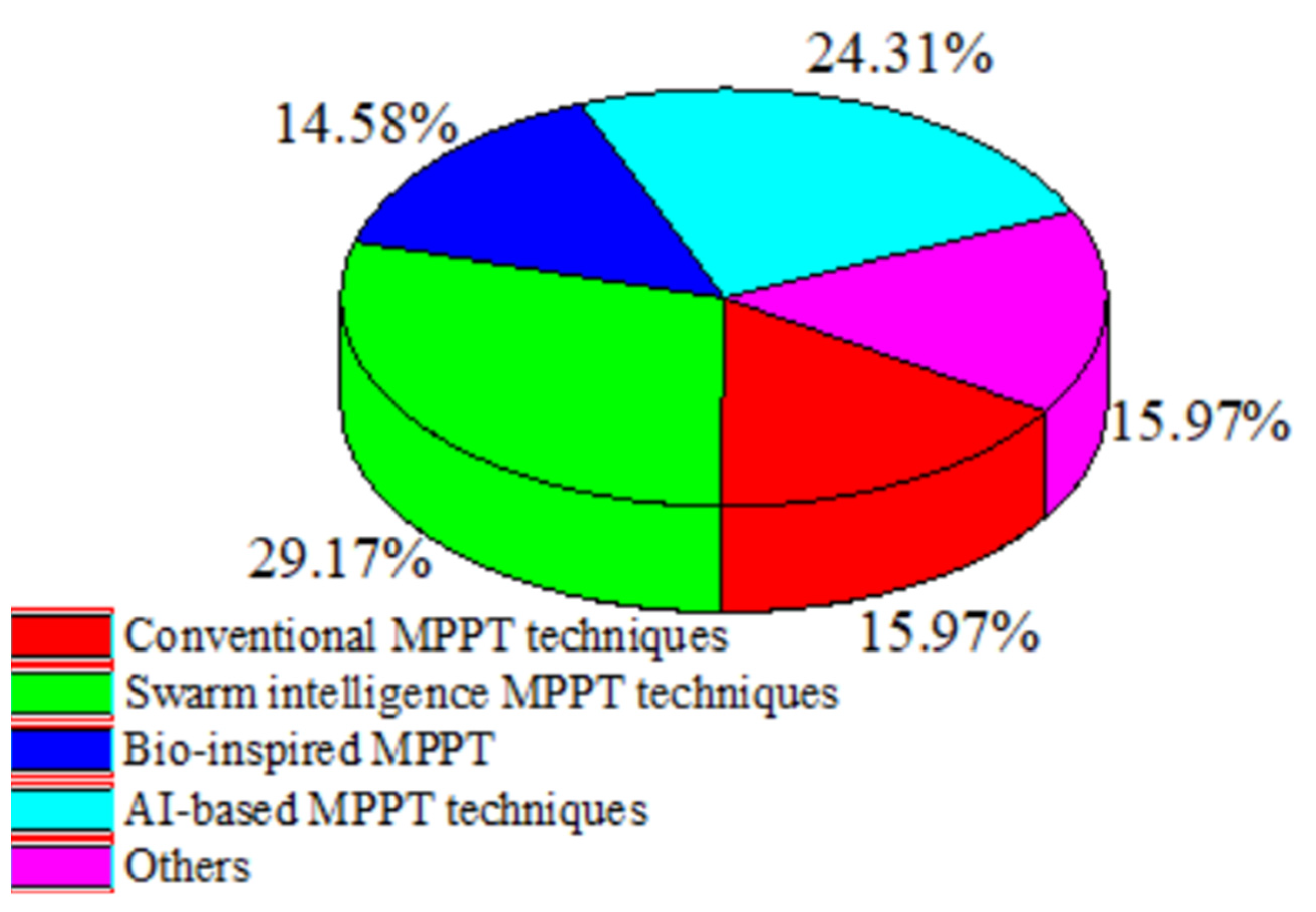
5. Research Gap and Findings
- Despite the fact that conventional techniques are simpler and work better in unshaded spaces, they have the downside of slow response. In their findings, oscillations around GMPP are observed;
- Even though these methods are frequently modified, power loss still occurs while monitoring open-circuit voltage or short-circuit current. Additionally, these methods need a large number of sensors to function, but those numbers can be decreased;
- In PSCs, AI approaches are effective, but they have the disadvantage of having high computational complexity;
- These methods require a great deal of time to track GMPP because of the large number of iterations. Despite the fact that many of these are only tested on virtual platforms, real-world validation is still crucial;
- Most of the reported work ignores the effect of load variation, which is crucial for building any PV system.
6. Challenges and Future Work
7. Conclusions
Author Contributions
Funding
Data Availability Statement
Acknowledgments
Conflicts of Interest
Abbreviations
| MPPT | Maximum power point tracking | PV | Photovoltaic |
| PSCs | Partial shading conditions | RES | Renewable energy sources |
| P–V | Power–voltage | GMPP | Global maximum power point |
| P&O | Perturb and observe | INC | Incremental conductance |
| HC | Hill climbing | BI | Bio-inspired |
| SI | Swarm intelligence | AI | Artificial intelligence |
| ANN | Artificial neural networks | FLC | Fuzzy logic control |
| ECI | Evolutionary computational intelligence | I–V | Current–voltage |
| MPP | Maximum power point | LMPP | Local maximum power points |
| DC | Direct current | CS | Cuckoo search |
| FOCV | Fractional open-circuit voltage | FSCC | Fractional short-circuit current |
| ACO | Ant colony optimization | ACO-P&O | Ant colony optimization–perturb and observe |
| SP-INC | Self-predictive incremental conductance | SPC | Semi pilot cell |
| PC | Pilot cell | CSAM | Current Sensorless Method with Auto-modulation |
| VSS | Variable step size | PSO | Particle swarm optimization |
| ABC | Artificial Bee Colony | GWO | Grey wolf optimization |
| SSA | Salp swarm algorithm | APSO | Accelerated PSO |
| LIPSO | Lagrange interpolation PSO | TS | Takagi–Sugeno |
| VCPSO | Variable coefficients PSO | CFPSO | Constriction factor-based PSO |
| OD-PSO | Overall distribution PSO | P&O-PSO | Perturb and observe-PSO |
| EGWO | Enhanced GWO | GWO-GSO | GWO–golden-section optimization |
| GWO-P&O | GWO–Perturb and observe | GOA | Grasshopper optimization algorithm |
| BOA | Bat algorithm | SSPSO | Series salp PSO |
| FA | Firefly elgorithm | ISSA | Improved salp swarm algorithm |
| DE | Differential Evolution | WOA | Whale optimization algorithm |
| SSO | Salp swarm optimization | ISSA | Improved salp swarm algorithm |
| SSPO | Hybrid salp swarm–perturb and observe | ABC-P&O | Artificial bee colony–perturb and observe |
| GMPPT | Global maximum power point tracking | MABC | Modified artificial bee colony |
| AIC | Angle of incremental conductance | IPSO | Improved particle swarm optimization |
| OGWO | Opposition-based learning GWO | DFO | Dragonfly optimization |
| TSA-PSO | Tunicate swarm algorithm with PSO | IABC | Improved artificial bee colony |
| SPF-P&O | Surface-sased polynomial fitting P&O | HGWO | Hybrid grey wolf optimization |
| DSM | Dynamic safty margin | ICPSO | Incremental conductance-based PSO |
| FSSO | Flying squirrel search optimization | BS | Best solution |
Nomenclature
| PV output current | |
| Photocurrent | |
| Shunt current | |
| Diode current | |
| Diode reverses saturation current | |
| Electron charge | |
| Number of cells in series | |
| Boltzmann constant | |
| Temperature | |
| PV output voltage | |
| Series resistance | |
| Shunt resistance | |
| Maximum power | |
| Open-circuit voltage | |
| Short-circuit current | |
| Change in power | |
| Change in voltage | |
| Change in current | |
| Voltage at maximum power point | |
| Proportionality constant | |
| Current at maximum power point | |
| Constant current factor | |
| Maximum power | |
| Gaussian kernel solution | |
| Sub-Gaussian function | |
| Mean value | |
| Standard deviation | |
| Weight factor | |
| Best optimal operating solution | |
| Convergence rate | |
| Individual best position | |
| Swarm optimum position | |
| particle position | |
| particle velocity | |
| Inertia burden | |
| Social and cognitive acceleration coefficients | |
| Arbitrary variables that are uniformly distributed between zero and one in terms of their assessments | |
| Target function | |
| -dimension maximum and minimum values. | |
| Arbitrarily selected food source | |
| Arbitrary number between | |
| Prey vector | |
| Position vector of grey wolf | |
| Coefficient vectors | |
| Random variables | |
| -rationalized candidate solution | |
| Position of food source | |
| Decemberision variables maximum and minimum value | |
| Initial call | |
| fireflies spatial coordinate components | |
| Step length | |
| Variance | |
| Maximum and minimum duty cycle | |
| Squirrels’ posture address at hickory and acorn trees | |
| Hovering constant (~1.90) | |
| Hovering distance | |
| PV output power | |
| Maximum voltage | |
| Hidden neuron numbers | |
| Injected input neurons numbers | |
| Output neurons numbers | |
| Instruction samples numbers |
References
- Kermadi, M.; Salam, Z.; Eltamaly, A.M.; Ahmed, J.; Mekhilef, S.; Larbes, C.; Berkouk, E.M. Recent Developments of MPPT Techniques for PV Systems under Partial Shading Conditions: A Critical Review and Performance Evaluation. IET Renew. Power Gener. 2020, 17, 3401–3417. [Google Scholar] [CrossRef]
- Singh, N.; Goswami, A. Study of P-V and I-V Characteristics of Solar Cell in MATLAB/Simulink. Int. J. Pure Appl. Math. 2018, 118, 24. [Google Scholar]
- Selvan, S.; Nair, P.; Umayal, A. Review on Photo Voltaic MPPT Algorithms. Int. J. Electr. Comput. Eng. 2016, 6, 567–582. [Google Scholar]
- Xu, L.; Cheng, R.; Yang, J. A New MPPT Technique for Fast and Efficient Tracking under Fast Varying Solar Irradiation and Load Resistance. Int. J. Photoenergy 2020, 2020, 6535372. [Google Scholar] [CrossRef]
- Gupta, A.K.; Chauhan, Y.K.; Pachauri, R.K. A comparative investigation of maximum power point tracking methods for solar PV system. Sol. Energy 2016, 136, 236–253. [Google Scholar] [CrossRef]
- Baba, A.O.; Liu, G.; Chen, X. Classification and Evaluation Review of Maximum Power Point Tracking Methods. Sustain. Futures 2020, 2, 100020. [Google Scholar] [CrossRef]
- Belhachat, F.; Larbes, C. A review of global maximum power point tracking techniques of photovoltaic system under partial shading conditions. Renew. Sustain. Energy Rev. 2018, 92, 513–553. [Google Scholar] [CrossRef]
- Podder, A.K.; Roy, N.K.; Pota, H.R. MPPT methods for solar PV systems: A critical review based on tracking nature. IET Renew. Power Gener. 2019, 13, 1615–1632. [Google Scholar] [CrossRef]
- Verma, D.; Nema, S.; Agrawal, R.; Sawle, Y.; Kumar, A. A Different Approach for Maximum Power Point Tracking (MPPT) Using Impedance Matching through Non-Isolated DC-DC Converters in Solar Photovoltaic Systems. Electronics 2022, 11, 1053. [Google Scholar] [CrossRef]
- Szemes, P.T.; Melhem, M. Analyzing and modeling PV with “P&O” MPPT Algorithm by MATLAB/SIMULINK. In Proceedings of the 3rd International Symposium on Small-Scale Intelligent Manufacturing Systems (SIMS) 2020, Gjovik, Norway, 10–12 June 2020; pp. 1–6. [Google Scholar]
- Christopher, I.W.; Ramesh, R. Comparative Study of P&O and InC MPPT Algorithms. Am. J. Eng. Res. 2013, 2, 402–408. [Google Scholar]
- Jately, V.; Azzopardi, B.; Joshi, J.; Venkateswaran, B.V.; Sharma, A.; Arora, S. Experimental Analysis of hill-climbing MPPT algorithms under low irradiance levels. Renew. Sustain. Energy Rev. 2021, 150, 111467. [Google Scholar] [CrossRef]
- Ali, A.; Almutairi, K.; Padmanaban, S.K.; Tirth, V.; Algarni, S.; Irshad, K.; Islam, S.; Zahir, M.H.; Shafiullah, M.; Malik, M.Z. Investigation of mppt techniques under uniform and non-uniform solar irradiation condition-a retrospection. IEEE Access 2020, 8, 127368–127392. [Google Scholar] [CrossRef]
- Batarseh, M.G.; Za’ter, M.E. Hybrid maximum power point tracking techniques: A comparative survey, suggested classification and uninvestigated combinations. Sol. Energy 2018, 169, 535–555. [Google Scholar] [CrossRef]
- Sundareswaran, K.; Vigneshkumar, V.; Palani, S. Development of a hybrid genetic algorithm/perturb and observe algorithm for maximum power point tracking in photovoltaic systems under non-uniform insolation. IET Renew. Power Gener. 2015, 9, 757–765. [Google Scholar] [CrossRef]
- Li, G.; Jin, Y.; Akram, M.W.; Chen, X.; Ji, J. Application of bio-inspired algorithms in maximum power point tracking for PV systems under partial shading conditions—A review. Renew. Sustain. Energy Rev. 2018, 81, 840–873. [Google Scholar] [CrossRef]
- Pathy, S.; Subramani, C.; Sridhar, R.; Thentral, T.M.T.; Padmanaban, S. Nature-Inspired MPPT Algorithms for Partially Shaded PV Systems: A Comparative Study. Energies 2019, 12, 1451. [Google Scholar] [CrossRef] [Green Version]
- Pilakkat, D.; Kanthalakshmi, S.; Navaneethan, S. A comprehensive review of swarm optimization algorithms for MPPT control of PV systems under partially shaded conditions. Electronics 2020, 24, 3–14. [Google Scholar] [CrossRef]
- Rezk, H.; Fathy, A.; Abdelaziz, A.Y. A comparison of different global MPPT techniques based on meta-heuristic algorithms for photovoltaic system subjected to partial shading conditions. Renew. Sustain. Energy Rev. 2017, 74, 377–386. [Google Scholar] [CrossRef]
- Tamrakar, R.; Gupta, A. A Review: Extraction of solar cell modelling parameters. Int. J. Innov. Res. Electr. Electron. Instrum. Control Eng. 2015, 3, 55–60. [Google Scholar]
- Singh, P.; Vinay, T.R.; Balyan, A.; Gangadhara; Sandeep, P.M. P-V and I-V Characteristics of Solar Cell. Design Eng. 2021, 6, 520–528. [Google Scholar]
- Bayrak, F.; Ertürk, G.; Oztop, H.F. Effects of partial shading on energy and exergy efficiencies for photovoltaic panels. J. Clean. Prod. 2017, 164, 58–69. [Google Scholar] [CrossRef]
- Nkambule, M.; Hasan, A.; Ali, J.A. Proportional study of Perturb & Observe and Fuzzy Logic Control MPPT Algorithm for a PV system under different weather conditions. In Proceedings of the IEEE 10th GCC Conference and Exhibition, Kuwait City, Kuwait, 19–23 April 2019. [Google Scholar]
- Reddy, D.C.K.; Satyanarayana, S.; Ganesh, V. Design of Hybrid Solar Wind Energy System in a Microgrid with MPPT Techniques. Int. J. Electr. Comput. Eng. 2018, 8, 730–740. [Google Scholar]
- Hajighorbani, S.; Amran, M.; Radzi, M.; Kadir, M.Z.A.A.; Shafie, S. Dual Search Maximum Power Point (DSMPP) Algorithm Based on Mathematical Analysis under Shaded Conditions. Energies 2015, 8, 12116–12146. [Google Scholar] [CrossRef] [Green Version]
- Ahmed, J.; Salam, Z. A Modified P&O Maximum Power Point Tracking Method with Reduced Steady-State Oscillation and Improved Tracking Efficiency. IEEE Trans. Sustain. Energy 2016, 7, 1506–1515. [Google Scholar]
- Sera, D.; Kerekes, T.; Teodorescu, R.; Blaabjerg, F. Improved MPPT Algorithms for Rapidly Changing Environmental Conditions. In Proceedings of the 2006 12th International Power Electronics and Motion Control Conference, Portoroz, Slovenia, 30 August–1 September 2006; pp. 1614–1619. [Google Scholar]
- Bouksaim, M.; Mekhfioui, M.; Srifi, M.N. Design and Implementation of Modified INC, Conventional INC, and Fuzzy Logic Controllers Applied to a PV System under Variable Weather Conditions. Designs 2021, 5, 71. [Google Scholar] [CrossRef]
- Babu, C.S.; Kumari, J.S.; Kullayappa, T.R. Design and Analysis of Open Circuit Voltage Based Maximum Power Point Tracking for Photovoltaic System. Int. J. Adv. Sci. Technol. 2011, 2, 51–60. [Google Scholar]
- Kumari, J.S.; Ch, S.B.; Yugandhar, J. Design and Investigation of Short Circuit Current Based Maximum Power Point Tracking for Photovoltaic System. Int. J. Res. Rev. Electr. Comput. Eng. 2011, 1, 63–68. [Google Scholar]
- Numan, B.A.; Shakir, A.M.; Ahmed, B.M. Enhancement of P&O algorithm for MPPT for partially shading PV systems. In Proceedings of the Academicsera International Conference, Antalya, Turkey, 21–22 January 2021. [Google Scholar]
- Gil-Velasco, A.; Aguilar-Castillo, C. A modification of the perturb and observe method to improve the energy harvesting of PV systems under partial shading conditions. Energies 2021, 14, 2521. [Google Scholar] [CrossRef]
- Efendi, M.Z.; Suhariningsih Murdianto, F.D.; Inawati, E. Implementation of modified P&O method as power optimizer of solar panel under partial shading condition for battery charging system. AIP Conf. Proc. 2018, 1977, 020002. [Google Scholar]
- Shang, L.; Guo, H.; Zhu, W. An improved MPPT control strategy based on incremental conductance algorithm. Prot. Control. Mod. Power Syst. 2020, 5, 14. [Google Scholar] [CrossRef]
- Zand, S.J.; Hsia, K.H.; Eskandarian, N.; Mobayen, S. Improvement of Self-Predictive Incremental Conductance Algorithm with the Ability to Detect Dynamic Conditions. Energies 2021, 14, 1234. [Google Scholar] [CrossRef]
- Baimel, D.; Tapuchi, S.; Levron, Y.; Belikov, J. Improved fractional open circuit voltage MPPT methods for PV systems. Electronics 2019, 8, 321–340. [Google Scholar] [CrossRef] [Green Version]
- Hua, C.; Chen, W.; Fang, Y. A hybrid MPPT with adaptive step-size based on single sensor for photovoltaic systems. In Proceedings of the 2014 International Conference on Information Science, Electronics and Electrical Engineering, Sapporo, Japan, 26–28 April 2014; pp. 441–445. [Google Scholar]
- Nadeem, A.; Sher, H.A.; Murtaza, A.F. Online fractional open-circuit voltage maximum output power algorithm for photovoltaic modules. IET Renew. Power Gener. 2020, 14, 188–198. [Google Scholar] [CrossRef]
- Fapi, C.B.N.; Wira, P.; Kamta, M. Real-time experimental assessment of a new MPPT algorithm based on the direct detection of the short-circuit current for a PV system. In Proceedings of the 19th International Conference on Renewable Energies and Power Quality (ICREPQ’21), Almeria, Spain, 28–30 July 2021. [Google Scholar]
- Sarika, E.P.; Jacob, J.; Mohammed, S.; Paul, S. A novel hybrid maximum power point tracking technique with zero oscillation based on P&O algorithm. Int. J. Renew. Energy Res. 2020, 10, 1962–1973. [Google Scholar]
- Li, C.; Chen, Y.; Zhou, D.; Liu, J.; Zeng, J. A High-Performance Adaptive Incremental Conductance MPPT Algorithm for Photovoltaic Systems. Energies 2016, 9, 288. [Google Scholar] [CrossRef] [Green Version]
- Owusu-Nyarko, I.; Elgenedy, M.A.; Abdelsalam, I.; Ahmed, K.H. Modified Variable Step-Size Incremental Conductance MPPT Technique for Photovoltaic Systems. Electronics 2021, 10, 2331. [Google Scholar] [CrossRef]
- Sarwar, S.; Javed, M.Y.; Jaffery, M.H.; Arshad, J.; Ur Rehman, A.; Shafiq, M.; Choi, J.-G. A Novel Hybrid MPPT Technique to Maximize Power Harvesting from PV System under Partial and Complex Partial Shading. Appl. Sci. 2022, 12, 587. [Google Scholar] [CrossRef]
- Hafeez, M.A.; Naeem, A.; Akram, M.; Javed, M.Y.; Asghar, A.B.; Wang, Y. A Novel Hybrid MPPT Technique Based on Harris Hawk Optimization (HHO) and Perturb and Observer (P&O) under Partial and Complex Partial Shading Conditions. Energies 2022, 15, 5550. [Google Scholar]
- González-Castaño, C.; Restrepo, C.; Revelo-Fuelagán, J.; Lorente-Leyva, L.L.; Peluffo-Ordóñez, D.H. A Fast-Tracking Hybrid MPPT Based on Surface-Based Polynomial Fitting and P&O Methods for Solar PV under Partial Shaded Conditions. Mathematics 2021, 9, 2732. [Google Scholar]
- Verma, P.; Alam, A.; Sarwar, A.; Tariq, M.; Vahedi, H.; Gupta, D.; Ahmad, S.; Mohamed, A.S.N. Meta-Heuristic optimization techniques used for maximum power point tracking in solar PV system. Electronics 2021, 10, 2419. [Google Scholar] [CrossRef]
- Jiang, L.L.; Maskell, D.L.; Patra, J.C. A novel ant colony optimization-based maximum power point tracking for photovoltaic systems under partially shaded conditions. Energy Build. 2013, 58, 227–236. [Google Scholar] [CrossRef]
- Oliveira, F.M.; da Silva, S.A.O.; Durand, F.R.; Sampaio, L.P. Application of PSO method for maximum power point extraction in photovoltaic systems under partial shading conditions. In Proceedings of the 2015 IEEE 13th Brazilian Power Electronics Conference and 1st Southern Power Electronics Conference (COBEP/SPEC), Fortaleza, Brazil, 29 November–2 December 2015; pp. 1–6. [Google Scholar]
- Benyoucef, A.S.; Chouder, A.; Kara, K.; Silvestre, S.; Sahed, O.A. Artificial bee colony based algorithm for maximum power point tracking (MPPT) for PV systems operating under partial shaded conditions. Appl. Soft Comput. 2015, 32, 38–48. [Google Scholar] [CrossRef] [Green Version]
- Mohapatra, A.; Nayak, B.; Das, P.; Mohanty, K.B. A review on MPPT techniques of PV system under partial shading condition. Renew. Sustain. Energy Rev. 2017, 80, 854–867. [Google Scholar] [CrossRef]
- Rezaei, H.; Bozorg-Haddad, O.; Chu, X. Grey Wolf Optimization (GWO) Algorithm. In Studies in Computational Intelligence; Springer: Berlin/Heidelberg, Germany, 2017; pp. 81–91. [Google Scholar]
- Mohanty, S.; Subudhi, B.; Ray, P.K. A New MPPT Design Using Grey Wolf Optimization Technique for Photovoltaic System Under Partial Shading Conditions. IEEE Trans. Sustain. Energy 2016, 7, 181–188. [Google Scholar] [CrossRef]
- Faris, H.; Mirjalili, S.; Aljarah, I.; Mafarja, M.; Heidari, A.A. Salp Swarm Algorithm: Theory, Literature Review, and Application in Extreme Learning Machines. In Nature-Inspired Optimizers. Studies in Computational Intelligence; Springer: Cham, Switzerland, 2019; Volume 811, pp. 185–199. [Google Scholar]
- Krishnan, G.S.; Kinattingal, S.; Simon, S.P.; Nayak, P.S.R. MPPT in PV systems using ant colony optimisation with dwindling population. IET Renew. Power Gener. 2020, 14, 1105–1112. [Google Scholar] [CrossRef]
- Sridhar, R.; Vishnuram, P.; Bindu, D.H.; Divya, A. Ant Colony Optimization based Maximum Power Point Tracking (MPPT) for Partially Shaded Standalone PV System. IJCTA 2016, 9, 8125–8133. [Google Scholar]
- Alshareef, M.; Lin, Z.; Ma, M.; Cao, W. Accelerated Particle Swarm Optimization for Photovoltaic Maximum Power Point Tracking under Partial Shading Conditions. Energies 2019, 12, 623. [Google Scholar] [CrossRef] [Green Version]
- Panda, K.P.; Anand, A.; Bana, P.R.; Panda, G. Novel PWM Control with Modified PSO-MPPT Algorithm for Reduced Switch MLI Based Standalone PV System. Int. J. Emerg. Electr. Power Syst. 2018, 19, 20180023. [Google Scholar] [CrossRef]
- Gopalakrishnan, S.K.; Kinattingal, S.; Simon, S.P. MPPT in PV Systems Using PSO Appended with Centripetal Instinct Attribute. Electr. Power Compon. Syst. 2020, 48, 881–891. [Google Scholar] [CrossRef]
- Mao, M.; Zhang, L.; Duan, Q.; Oghorada, O.J.K.; Duan, P.; Hu, B. A Two-Stage Particle Swarm Optimization Algorithm for MPPT of Partially Shaded PV Arrays. Int. J. Green Energy 2017, 4, 694–702. [Google Scholar] [CrossRef]
- Koad, R.B.A.; Zobaa, A.F.; El-Shahat, A. A Novel MPPT Algorithm Based on Particle Swarm Optimization for Photovoltaic Systems. IEEE Trans. Sustain. Energy 2017, 8, 468–476. [Google Scholar] [CrossRef] [Green Version]
- Belghith, O.B.; Sbita1, L.; Bettaher, F. MPPT Design Using PSO Technique for Photovoltaic System Control Comparing to Fuzzy Logic and P&O Controllers. Energy Power Eng. 2016, 8, 349–366. [Google Scholar]
- Obukhov, S.; Ibrahim, A.; Zaki Diab, A.A.; Al-Sumaiti, A.S.; Aboelsaud, R. Optimal Performance of Dynamic Particle Swarm Optimization Based Maximum Power Trackers for Stand-Alone PV System Under Partial Shading Conditions. IEEE Access 2020, 8, 20770–20785. [Google Scholar] [CrossRef]
- Li, H.; Yang, D.; Su, W.; Lü, J.; Yu, X. An Overall Distribution Particle Swarm Optimization MPPT Algorithm for Photovoltaic System Under Partial Shading. IEEE Trans. Ind. Electron. 2019, 66, 265–275. [Google Scholar] [CrossRef]
- Suhardi, D.; Syafaah, L.; Irfan, M.; Yusuf, M.; Effendy, M.; Pakaya, I. Improvement of maximum power point tracking (MPPT) efficiency using grey wolf optimization (GWO) algorithm in photovoltaic (PV) system. IOP Conf. Ser. Mater. Sci. Eng. 2019, 674, 012038. [Google Scholar] [CrossRef]
- Kumar, C.S.; Rao, R.S. Enhanced Grey Wolf Optimizer Based MPPT Algorithm of PV System Under Partial Shaded Condition. Int. J. Renew. Energy Dev. 2017, 6, 203–212. [Google Scholar]
- Shi, J.Y.; Zhang, D.Y.; Ling, L.T.; Xue, F.; Li, Y.J.; Qin, Z.J.; Yang, T. Dual-Algorithm Maximum Power Point Tracking Control Method for Photovoltaic Systems based on Grey Wolf Optimization and Golden-Section Optimization. J. Power Electron. 2018, 18, 841–852. [Google Scholar]
- Ilyas, M.; Ghazal, H.K.E. Design of a MPPT System Based on Modified Grey Wolf Optimization Algorithm in Photovoltaic System under Partially Shaded Condition. Int. J. Comput. 2021, 40, 36–49. [Google Scholar]
- Kraiem, H.; Aymen, F.; Yahya, L.; Triviño, A.; Alharthi, M.; Ghoneim, S.S.M. A Comparison between Particle Swarm and GreyWolf Optimization Algorithms for Improving the Battery Autonomy in a Photovoltaic System. Appl. Sci. 2021, 11, 7732. [Google Scholar] [CrossRef]
- Jamaludin, M.N.I.; Tajuddin, M.F.N.; Ahmed, J.; Azmi, A.; Azmi, S.A.; Ghazali, N.H.; Babu, T.S.; Alhelou, H.H. An Effective Salp Swarm Based MPPT for Photovoltaic Systems Under Dynamic and Partial Shading Conditions. IEEE Access 2021, 9, 34570–34589. [Google Scholar] [CrossRef]
- Dagal, I.; Akın, B.; Akboy, E. A novel hybrid series salp particle Swarm optimization (SSPSO) for standalone battery charging applications. Ain Shams Eng. J. 2022, 13, 101747. [Google Scholar] [CrossRef]
- Krishnan, S.; Sathiyasekar, K. A Novel Salp Swarm Optimization MPP Tracking Algorithm for the Solar Photovoltaic Systems under Partial Shading Conditions. J. Circuits Syst. Comput. 2020, 29, 2050017. [Google Scholar] [CrossRef]
- Farzaneh, J.; Karsaz, A. Application of Improved Salp Swarm Algorithm Based on MPPT for PV Systems under Partial Shading Conditions. Int. J. Ind. Electron. Control Optim. 2020, 3, 415–429. [Google Scholar]
- Ali, M.H.M.; Mohamed, M.M.S.; Ahmed, N.M.; Zahran, M.B.A. Comparison between P&O and SSO techniques based MPPT algorithm for photovoltaic systems. Int. J. Electr. Comput. Eng. 2022, 12, 32–40. [Google Scholar]
- Balaji, V.; Fathima, A.P. Enhancing the Maximum Power Extraction in Partially Shaded PV Arrays Using Hybrid Salp Swarm Perturb and Observe Algorithm. Int. J. Renew. Energy Res. 2020, 10, 898–911. [Google Scholar]
- Restrepo, C.; Yanez-Monsalvez, N.; González-Castaño, C.; Kouro, S.; Rodriguez, J. A Fast Converging Hybrid MPPT Algorithm Based on ABC and P&O Techniques for a Partially Shaded PV System. Mathematics 2021, 9, 2228. [Google Scholar]
- Sawant, P.T.; Tejasvi, P.C.; Bhattar, L.; Bhattar, C.L. Enhancement of PV System Based on Artificial Bee Colony Algorithm under dynamic Conditions. In Proceedings of the IEEE International Conference on Recent Trends In Electronics Information Communication Technology 2016, Bangalore, India, 20–21 May 2016; pp. 1251–1255. [Google Scholar]
- Li, N.; Mingxuan, M.; Yihao, W.; Lichuang, C.; Lin, Z.; Qianjin, Z. Maximum Power Point Tracking Control Based on Modified ABC Algorithm for Shaded PV System. In Proceedings of the 2019 AEIT International Conference of Electrical and Electronic Technologies for Automotive (AEIT AUTOMOTIVE), Turin, Italy, 2–4 July 2019; pp. 1–5. [Google Scholar]
- Wan, Y.; Mao, M.; Zhou, L.; Zhang, Q.; Xi, X.; Zheng, C. A Novel Nature-Inspired Maximum Power Point Tracking (MPPT) Controller Based on SSA-GWO Algorithm for Partially Shaded Photovoltaic Systems. Electronics 2019, 8, 680. [Google Scholar] [CrossRef] [Green Version]
- Hayder, W.; Ogliari, E.; Dolara, A.; Abid, A.; Hamed, M.B.; Sbita, L. Improved PSO: A Comparative Study in MPPT Algorithm for PV System Control under Partial Shading Conditions. Energies 2020, 13, 2035. [Google Scholar] [CrossRef]
- Almutairi, A.; Abo-Khalil, A.G.; Sayed, K.; Albagami, N. MPPT for a PV Grid-Connected System to Improve efficiency under Partial Shading Conditions. Sustainability 2020, 12, 10310. [Google Scholar] [CrossRef]
- Sharma, A.; Sharma, A.; Jately, V.; Averbukh, M.; Rajput, S.; Azzopardi, B. A Novel TSA-PSO Based Hybrid Algorithm for GMPP Tracking under Partial Shading Conditions. Energies 2022, 15, 3164. [Google Scholar] [CrossRef]
- Chao, K.-H.; Li, J.-Y. Global Maximum Power Point Tracking of Photovoltaic Module Arrays Based on Improved Artificial Bee Colony Algorithm. Electronics 2022, 11, 1572. [Google Scholar] [CrossRef]
- Alaraj, M.; Kumar, A.; Alsaidan, I.; Rizwan, M.; Jamil, M. An Advanced and Robust Approach to Maximize Solar Photovoltaic Power Production. Sustainability 2022, 14, 7398. [Google Scholar] [CrossRef]
- Windarko, N.A.; Nizar Habibi, M.; Sumantri, B.; Prasetyono, E.; Efendi, M.Z.; Taufik, A. New MPPT Algorithm for Photovoltaic Power Generation under Uniform and Partial Shading Conditions. Energies 2021, 14, 483. [Google Scholar] [CrossRef]
- Chawda, G.S.; Mahela, O.P.; Gupta, N.; Khosravy, M.; Senjyu, T. Incremental Conductance Based Particle Swarm Optimization Algorithm for Global Maximum Power Tracking of Solar-PV under Nonuniform Operating Conditions. Appl. Sci. 2020, 10, 4575. [Google Scholar] [CrossRef]
- Teshome, D.F.; Lee, C.H.; Lin, Y.W.; Lian, K.L. A Modified Firefly Algorithm for Photovoltaic Maximum Power Point Tracking Control Under Partial Shading. IEEE J. Emerg. Sel. Top. Power Electron. 2017, 5, 661–671. [Google Scholar] [CrossRef]
- Nugraha, D.A.; Lian, K.L.; Suwarno. A Novel MPPT Method Based on Cuckoo Search Algorithm and Golden Section Search Algorithm for Partially Shaded PV System. Can. J. Electr. Comput. Eng. 2019, 42, 173–182. [Google Scholar] [CrossRef]
- Assis, A.; Mathew, S. Cuckoo Search Algorithm Based Maximum Power Point Tracking For Solar PV Systems. Int. J. Adv. Electr. Power Syst. Inf. Technol. 2016, 2, 20–28. [Google Scholar]
- Jain, M.; Singh, V.; Rani, A. A novel nature-inspired algorithm for optimization: Squirrel search algorithm. Swarm and Evolutionary Computation 2019, 44, 148–175. [Google Scholar] [CrossRef]
- Saad, W.; Hegazy, E.; Shokair, M. Maximum power point tracking based on modified firefly scheme for PV system. SN Appl. Sci. 2022, 4, 94. [Google Scholar] [CrossRef]
- Farzaneh, J.; Keypour, R.; Khanesar, M.A. A New Maximum Power Point Tracking Based on Modified Firefly Algorithm for PV System Under Partial Shading Conditions. Technol. Econ. Smart Grids Sustain. Energy 2018, 3, 9. [Google Scholar] [CrossRef] [Green Version]
- Nusaif, A.I.; Mahmood, A.L. MPPT Algorithms (PSO, FA, and MFA) for PV System Under Partial Shading Condition, Case Study: BTS in Algazalia, Baghdad. Int. J. Smart Grid 2020, 10, 100–110. [Google Scholar]
- Abo-Khalil, A.G.; Alharbi, W.; Al-Qawasmi, A.R.; Alobaid, M.; Alarifi, I.M. Maximum Power Point Tracking of PV Systems under Partial Shading Conditions Based on Opposition-Based Learning Firefly Algorithm. Sustainability 2021, 13, 2656. [Google Scholar] [CrossRef]
- Shi, J.-Y.; Ling, L.-T.; Xue, F.; Qin, Z.-J.; Li, Y.-J.; Lai, Z.-X.; Yang, T. Combining incremental conductance and firefly algorithm for tracking the global MPP of PV arrays. J. Renew. Sustain. Energy 2017, 9, 023501. [Google Scholar] [CrossRef]
- Omar, F.A.; Kulaksiz, A.A. Experimental evaluation of a hybrid global maximum power tracking algorithm based on modified firefly and perturbation and observation algorithms. Neural Comput. Appl. 2021, 33, 17185–17208. [Google Scholar] [CrossRef]
- Chitra, A.; Yogitha, G.; Sivaramakrishnan, K.; Sultana, W.R.; Sanjeevikumar, P. Modified Firefly-Based Maximum Power Point Tracking Algorithm for PV Systems Under Partial Shading Conditions. In Artificial Intelligent Techniques for Electric and Hybrid Electric Vehicles; Scrivener Publishing LLC: Beverly, MA, USA, 2020; pp. 143–164. [Google Scholar]
- Mosaad, M.I.; Abed el-Raouf, M.O.; Al-Ahmar, M.A.; Banakher, F.A. Maximum Power Point Tracking of PV system Based Cuckoo Search Algorithm; review and comparison. Energy Procedia 2019, 162, 117–126. [Google Scholar] [CrossRef]
- Shi, Y.-J.; Xue, F.; Qin, Z.-J.; Zhang, W.; Ling, L.-T.; Yang, T. Improved Global Maximum Power Point Tracking for Photovoltaic System via Cuckoo Search under Partial Shaded Conditions. J. Power Electron. 2016, 16, 287–296. [Google Scholar] [CrossRef] [Green Version]
- Hidayat, T.; Efendi, M.Z.; Murdianto, F.D. Maximum Power Point Tracking Interleaved Boost Converter Using Cuckoo Search Algorithm on The Nano Grid System. J. Adv. Res. Electr. Eng. 2021, 5, 41–46. [Google Scholar] [CrossRef]
- Bilgin, N.; Yazici, I. Comparison of Maximum Power Point Tracking Methods Using Metaheuristic Optimization Algorithms for Photovoltaic Systems. Sak. Univ. J. Sci. 2021, 25, 1075–1085. [Google Scholar] [CrossRef]
- Ibrahim, A.-W.; Fang, Z.; Ameur, K.; Min, D.; Shafik, M.B.; Al-Muthanna, G. Comparative Study of Solar PV System Performance under Partial Shaded Condition Utilizing Different Control Approaches. Indian J. Sci. Technol. 2021, 14, 1864–1893. [Google Scholar] [CrossRef]
- Bentata, K.; Mohammedi, A.; Benslimane, T. Development of rapid and reliable cuckoo search algorithm for global maximum power point tracking of solar PV systems in partial shading condition. Arch. Control Sci. 2021, 31, 495–526. [Google Scholar]
- Singh, N.; Gupta, K.K.; Jain, S.K.; Dewangan, N.K.; Bhatnagar, P. A Flying Squirrel Search Optimization for MPPT Under Partial Shaded Photovoltaic System. IEEE J. Emerg. Sel. Top. Power Electron. 2021, 9, 4963–4978. [Google Scholar] [CrossRef]
- Fares, D.; Fathi, M.; Shams, I.; Mekhilef, S. A novel global MPPT technique based on squirrel search algorithm for PV module under partial shading conditions. Energy Convers. Manag. 2021, 230, 113773. [Google Scholar] [CrossRef]
- Al-Shammaa, A.A.; Abdurraqeeb, A.M.; Noman, A.M.; Alkuhayli, A.; Farh HM, H. Hardware-In-the-Loop Validation of Direct MPPT Based Cuckoo Search Optimization for Partially Shaded Photovoltaic System. Electronics 2022, 11, 1655. [Google Scholar] [CrossRef]
- Watanabe, R.B.; Ando Junior, O.H.; Leandro PG, M.; Salvadori, F.; Beck, M.F.; Pereira, K.; Brandt MH, M.; De Oliveira, F.M. Implementation of the Bio-Inspired Metaheuristic Firefly Algorithm (FA) Applied to Maximum Power Point Tracking of Photovoltaic Systems. Energies 2022, 15, 5338. [Google Scholar] [CrossRef]
- Pandey, A.K.; Singh, V.; Jain, S. Chapter eleven—Study and comparative analysis of perturb and observe (P&O) and fuzzy logic based PV-MPPT algorithms. In Applications of AI and IOT in Renewable Energy; Academic Press: Cambridge, MA, USA, 2022; pp. 193–209. [Google Scholar]
- Almajid, S.; Al-Raweshidy, H.; Abbod, M. A Novel Maximum Power Point Tracking Technique based on Fuzzy logic for Photovoltaic Systems. Int. J. Hydrogen Energy 2018, 43, 14158–14171. [Google Scholar] [CrossRef]
- Jyothy, L.P.N.; Sindhu, M.R. An Artificial Neural Network based MPPT Algorithm for Solar PV System. In Proceedings of the 4th International Conference on Electrical Energy Systems (ICEES), Chennai, India, 7–9 February 2018; pp. 375–380. [Google Scholar]
- Selivanov, S.G.; Poezjalova, S.N.; Gavrilova, O.A. The Use of Artificial Intelligence Methods of Technological Preparation of Engine-Building Production. Am. J. Ind. Eng. 2014, 2, 10–14. [Google Scholar]
- Verma, P.; Garg, R.; Mahajan, P. Asymmetrical fuzzy logic control-based MPPT algorithm for stand-alone photovoltaic systems under partially shaded conditions. Sci. Iran. 2020, 27, 3162–3174. [Google Scholar]
- Rahman, M.M.; Islam, M.S. PSO and ANN Based Hybrid MPPT Algorithm for Photovoltaic Array under Partial Shading Condition. Eng. Int. 2020, 8, 9–24. [Google Scholar] [CrossRef]
- Farzaneh, J. A Hybrid Modified FA-ANFIS-P&O Approach for MPPT in Photovoltaic Systems under PSCs. Int. J. Electron. 2019, 107, 703–718. [Google Scholar]
- Manikandan, P.V.; Selvaperuma, S. EANFIS-based Maximum Power Point Tracking for Standalone PV System. IETE J. Res. 2022, 68, 4218–4231. [Google Scholar] [CrossRef]
- Al-Majidi, S.D.; Abbod, M.F.; Al-Raweshidy, H.S. Design of an Efficient Maximum Power Point Tracker Based on ANFIS Using an Experimental Photovoltaic System Data. Electronics 2019, 8, 858. [Google Scholar] [CrossRef] [Green Version]
- Aymen, J.; Ons, Z.; Crăciunescu, A.; Popescu, M. Comparison of Fuzzy and Neuro-Fuzzy Controllers for Maximum Power Point Tracking of Photovoltaic Modules. Renew. Energy Power Qual. J. 2016, 1, 796–800. [Google Scholar] [CrossRef] [Green Version]
- Farajdadian, S.; Hosseini, S.M.H. Design of an optimal fuzzy controller to obtain maximum power in solar power generation system. Sol. Energy 2019, 182, 161–178. [Google Scholar] [CrossRef]
- Eltamalya, A.M.; Farh, H.M.H. Dynamic global maximum power point tracking of the PV systems under variant partial shading using hybrid GWO-FLC. Sol. Energy 2019, 177, 306–316. [Google Scholar] [CrossRef]
- Chen, Y.-T.; Jhang, Y.-C.; Liang, R.-H. A fuzzy-logic based auto-scaling variable step-size MPPT method for PV systems. Sol. Energy 2016, 126, 53–63. [Google Scholar] [CrossRef]
- Raj, A.; Gupta, M. Numerical Simulation and Performance Assessment of ANN-INC Improved Maximum Power Point Tracking System for Solar Photovoltaic System Under Changing Irradiation Operation. Ann. Rom. Soc. Cell Biol. 2021, 25, 790–797. [Google Scholar]
- Abdellatif, W.S.E.; Mohamed, M.S.; Barakat, S.; Brisha, A. A Fuzzy Logic Controller Based MPPT Technique for Photovoltaic Generation System. Int. J. Electr. Eng. Inform. 2021, 13, 394–417. [Google Scholar]
- Mohammed, S.S.; Devaraj, D.; Ahamed, T.P.I. GA-Optimized Fuzzy-Based MPPT Technique for Abruptly Varying Environmental Conditions. J. Inst. Eng. Ser. B 2021, 102, 497–508. [Google Scholar] [CrossRef]
- Tandel, B.G.; Vora, D.R. MPP Detection Based on Genetic Algorithm for PV System in Partial Shading Condition. Int. J. Res. Dev. Technol. 2016, 5, 107–115. [Google Scholar]
- Karthika, S.; Rathika, P.; Devaraj, D. Evaluation of GA Tuned PI Controller for Maximum Power Point Tracking for Solar PV System under Partially Shaded Conditions Based on Two Diode Model. World Appl. Sci. J. 2017, 35, 2580–2590. [Google Scholar]
- Dehghani, M.; Taghipour, M.; Gharehpetian, G.B.; Abedi, M. Optimized Fuzzy Controller for MPPT of Grid-connected PV Systems in Rapidly Changing Atmospheric Conditions. J. Mod. Power Syst. Clean Energy 2021, 9, 376–383. [Google Scholar] [CrossRef]
- Bendary, F.M.; Saied, E.M.; Mohamed, W.A.; Afifi, Z.E. Optimal Maximum Power Point Tracking of PV Systems based Genetic-ANFIS Hybrid Algorithm. Int. J. Sci. Eng. Res. 2016, 7, 830–836. [Google Scholar]
- Firmanza, A.P.; Habibi, M.N.; Windarko, N.A.; Yanaratri, D.S. Differential Evolution-based MPPT with Dual Mutation for PV Array under Partial Shading Condition. In Proceedings of the 2020 10th Electrical Power, Electronics, Communications, Controls and Informatics Seminar (EECCIS), Malang, Indonesia, 26–28 August 2020; pp. 198–203. [Google Scholar]
- Neethu, M.; Senthilkumar, R. Comparison Method of PSO and DE Optimization for MPPT in PV Systems under Partial Shading Conditions. Int. Energy J. 2020, 20, 291–298. [Google Scholar]
- Kamaruddina, N.I.; Haron, A.R.; Chua, B.L.; Tan, M.K.; Lim, K.G.; Teo, K.T.K. Differential Evolution Based Maximum Power Point Tracker for Photovoltaic Array Under Non-Uniform Illumination Condition. ICTACT J. Soft Comput. 2020, 10, 2076–2083. [Google Scholar]
- Joisher, M.; Singh, D.; Taheri, S.; Espinoza-Trejo, D.R.; Pouresmaeil, E.; Taheri, H. A Hybrid Evolutionary-Based MPPT for Photovoltaic Systems Under Partial Shading Conditions. IEEE Access 2020, 8, 38481–38492. [Google Scholar] [CrossRef]
- Algarín, C.R.; Giraldo, J.T.; Álvarez, O.R. Fuzzy Logic Based MPPT Controller for a PV System. Energies 2017, 10, 2036. [Google Scholar] [CrossRef] [Green Version]
- Cheng, P.-C.; Peng, B.-R.; Liu, Y.-H.; Cheng, Y.-S.; Huang, J.-W. Optimization of a Fuzzy-Logic-Control-Based MPPT Algorithm Using the Particle Swarm Optimization Technique. Energies 2015, 8, 5338–5360. [Google Scholar] [CrossRef] [Green Version]
- Liu, C.-L.; Chen, J.-H.; Liu, Y.-H.; Yang, Z.-Z. An Asymmetrical Fuzzy-Logic-Control-Based MPPT Algorithm for Photovoltaic Systems. Energies 2014, 7, 2177–2193. [Google Scholar] [CrossRef] [Green Version]
- Kececioglu, O.F.; Gani, A.; Sekkeli, M. Design and Hardware Implementation Based on Hybrid Structure for MPPT of PV System Using an Interval Type-2 TSK Fuzzy Logic Controller. Energies 2020, 13, 1842. [Google Scholar] [CrossRef] [Green Version]
- Hayder, W.; Sera, D.; Ogliari, E.; Lashab, A. On Improved PSO and Neural Network P&O Methods for PV System under Shading and Various Atmospheric Conditions. Energies 2022, 15, 7668. [Google Scholar]
- Hua, C.-C.; Zhan, Y.-J. A Hybrid Maximum Power Point Tracking Method without Oscillations in Steady-State for Photovoltaic Energy Systems. Energies 2021, 14, 5590. [Google Scholar] [CrossRef]
- Zhang, P.; Sui, H. Maximum Power Point Tracking Technology of Photovoltaic Array under Partial Shading Based on Adaptive Improved Di_erential Evolution Algorithm. Energies 2020, 13, 1254. [Google Scholar] [CrossRef] [Green Version]
- Bakkar, M.; Aboelhassan, A.; Abdelgeliel, M.; Galea, M. PV Systems Control Using Fuzzy Logic Controller Employing Dynamic Safety Margin under Normal and Partial Shading Conditions. Energies 2021, 14, 841. [Google Scholar] [CrossRef]
- Bataineh, K.; Eid, N. A Hybrid Maximum Power Point Tracking Method for Photovoltaic Systems for Dynamic Weather Conditions. Resources 2018, 7, 68. [Google Scholar] [CrossRef] [Green Version]
- Guerra MI, S.; Ugulino de Araújo, F.M.; Dhimish, M.; Vieira, R.G. Assessing Maximum Power Point Tracking Intelligent Techniques on a PV System with a Buck–Boost Converter. Energies 2021, 14, 7453. [Google Scholar] [CrossRef]
- Minai, A.F.; Khan, A.A.; Pachauri, R.K.; Malik, H.; Márquez, F.P.G.; Jiménez, A.A. Performance Evaluation of Solar PV-Based Z-Source Cascaded Multilevel Inverter with Optimized Switching Scheme. Electronics 2022, 11, 3706. [Google Scholar] [CrossRef]
- Minai, A.F.; Malik, H. Metaheuristics Paradigms for Renewable Energy Systems: Advances in Optimization Algorithms. Springer Nature Book: Metaheuristic and Evolutionary Computation: Algorithms and Applications. In Metaheuristic and Evolutionary Computation: Algorithms and Applications; Studies in Computational Intelligence; Springer: Singapore, 2020; pp. 35–61. [Google Scholar]
- Chankaya, M.; Hussain, I.; Ahmad, A.; Fausto, P.; García, M. Multi-Objective Grasshopper Optimization Based MPPT and VSC Control of Grid-Tied PV-Battery System. Electronics 2021, 10, 2770. [Google Scholar] [CrossRef]
- Tajjour, S.; Chandel, S.S.; Alotaibi, M.A.; Ustun, T.S.A. Novel Metaheuristic Approach for Solar Photovoltaic Parameter Extraction Using Manufacturer Data. Photonics 2022, 9, 858. [Google Scholar] [CrossRef]


| Authors [Reference No.] | Optimization Techniques | Best optimization Techniques | PV Module Pm (W) | PV System Size | GMPP (W) | Improved GMPP (%) | Irradiance (W/m2) | Shading Patterns | Tracking Time (s) |
|---|---|---|---|---|---|---|---|---|---|
| Numan BA et al. [31] | P&O Variable-step P&O | Variable-step P&O | 71.8 | 2 PV module in series | 29.22, 116.1, 106.2 | 0 | 200, 700, 800 | Uniform | 2, 4.8 |
| Gil-Velasco A et al. [32] | P&O, ACO, ACO-P&O, Proposed | Proposed | 250 | 5 PV module in series | 44.97, 30.49 | 102.9, 35.15 | 1000–200 | Uniform | 1.12 |
| Efendi MZ et al. [33] | P&O, Modified P&O | Modified P&O | 50 | 3 PV module in series | 6037, 5387, 7051, 7385,6322 | 8.30, 31.19, 61.42, 31.63, 27.69 | 946–828 | Uniform | NA |
| Shang L et al. [34] | Conventional INC Proposed INC | Proposed INC | 49.8 | 1 PV module | 25.1, 40.18 25.1, 27.61 | 0.039, 0.424, 0.199, 0.217 | 800–300 | Uniform | 0.3, 0.35, 0.16, 0.05 |
| Zand SJ et al. [35] | INC SP-INC | SP-INC | 100.17 | 1X1 | 98.981, 94.097, 81.292 | 1.811, 1.179, 1.615 | 1000–800 | Uniform | NA |
| Baimel D et al. [36] | FOCV PC SPC | SPC | NA | NA | 27.11, 15.76, 04.83 | 0.93, 11.01, 0.89 10.98, 0.83, 11.03 | 1000–200 | Uniform | NA |
| Hua C et al. [37] | CSAM Proposed | Proposed | 60 | 4 PV module in series | 470.95 | 7.27 | 1000–300 | Uniform | 0.043, 0.049 |
| Nadeem A et al. [38] | Analytical FOCV Offline FOCV, Proposed | Proposed | 245.328 | 3 PV module in series | 438.15 | 89.67, 0.51 | 1000–600 | Uniform | NA |
| Fapi CBN et al. [39] | FSCC, Proposed | Proposed | 145 | 1PV module | 85 | 13.33 | NA | NA | 0.7 |
| Sarika EP et al. [40] | Proposed, VSS P&O, VSS fuzzy | Proposed | 100 | 1PV module | 76.50, 65.27 | 4.08, 2.99 | 1000–600 | Non uniform | 0.01 |
| Li C et al. [41] | Proposed INC Fixed-step INC Variable-step INC | Proposed INC | 178.4 | NA | 175.6 | 1.738 | 1000–0 | Non uniform | 0.38, 0.14, 0.165 |
| Owusu-Nyarko I et al. [42] | Proposed, Variable-step-size methods | Proposed | 60 | NA | 596.9 | 0.285 | 1000–400 | Non uniform | 0.0126 |
| Sarwar S et al. [43] | PSO, DFO, INC, Hybrid, CS, FA, ACO | Hybrid | 315.072 | 4X1 | 511.4, 780.4 | 57.35, 9.6 | 1000–200 | Non uniform | 0.48, 0.20 |
| Hafeez M A et al. [44] | Hybrid, DFO, ACS, WCA, PSO, P&O. | Hybrid | NA | 4 PV module in series | 1259.9, 794.8, 593.2, 1077.0 | 1.933, 0.353, 7.32, 0.937 | 1000–200 | Non uniform | 0.16, 0.25, 0.4, 0.17 |
| González-Castaño C et al. [45] | SPF-P&O, P&O | SPF-P&O | 200 | 4 PV module in series | 405.63, 331.85 | 4.59, 30.53 | 1000–120 | Uniform & Non uniform | NA |
| Authors [Reference No.] | Pros | Cons |
|---|---|---|
| Numan BA et al. [31] |
|
|
| Gil-Velasco A et al. [32] |
|
|
| Efendi MZ et al. [33] |
|
|
| Shang L et al. [34] |
|
|
| Zand SJ et al. [35] |
|
|
| Baimel D et al. [36] |
|
|
| Hua C et al. [37] |
|
|
| Nadeem A et al. [38] |
|
|
| Fapi CBN et al. [39] |
|
|
| Sarika EP et al. [40] |
|
|
| Li C et al. [41] |
|
|
| Owusu-Nyarko I et al. [42] |
|
|
| Sarwar S et al. [43] |
|
|
| Hafeez M A et al. [44] |
|
|
| González-Castaño C et al. [45] |
|
|
| Categorization | Technique | Execution Cost | Accuracy | Tracking Speed | Oscillations Around MPP | Computational Complexity | Analog/Digital | ||||||||||||
|---|---|---|---|---|---|---|---|---|---|---|---|---|---|---|---|---|---|---|---|
| L | M | H | L | M | H | L | M | H | L | M | H | ~Z | L | M | H | D | A/D | ||
| Conventional | P&O |  | | | | | | ||||||||||||
| INC | | | | | | | |||||||||||||
| FOCV | | | | | | | |||||||||||||
| FSCC | | | | | | | |||||||||||||
| AI-Based Metaheuristic techniques | ACO | | | | | | | ||||||||||||
| PSO | | | | | | | |||||||||||||
| ABC | | | | | | | |||||||||||||
| GWO | | | | | | | |||||||||||||
| SSA | | | | | | | |||||||||||||
| FFA | | | | | | | |||||||||||||
| CS | | | | | | | |||||||||||||
| FSSO | | | | | | | |||||||||||||
| Other AI | FLC | | | | | | | ||||||||||||
| ANN | | | | | | | |||||||||||||
| GA | | | | | | | |||||||||||||
| DE | | | | | | | |||||||||||||
Disclaimer/Publisher’s Note: The statements, opinions and data contained in all publications are solely those of the individual author(s) and contributor(s) and not of MDPI and/or the editor(s). MDPI and/or the editor(s) disclaim responsibility for any injury to people or property resulting from any ideas, methods, instructions or products referred to in the content. |
© 2023 by the authors. Licensee MDPI, Basel, Switzerland. This article is an open access article distributed under the terms and conditions of the Creative Commons Attribution (CC BY) license (https://creativecommons.org/licenses/by/4.0/).
Share and Cite
Sharma, A.K.; Pachauri, R.K.; Choudhury, S.; Minai, A.F.; Alotaibi, M.A.; Malik, H.; Márquez, F.P.G. Role of Metaheuristic Approaches for Implementation of Integrated MPPT-PV Systems: A Comprehensive Study. Mathematics 2023, 11, 269. https://doi.org/10.3390/math11020269
Sharma AK, Pachauri RK, Choudhury S, Minai AF, Alotaibi MA, Malik H, Márquez FPG. Role of Metaheuristic Approaches for Implementation of Integrated MPPT-PV Systems: A Comprehensive Study. Mathematics. 2023; 11(2):269. https://doi.org/10.3390/math11020269
Chicago/Turabian StyleSharma, Amit Kumar, Rupendra Kumar Pachauri, Sushabhan Choudhury, Ahmad Faiz Minai, Majed A. Alotaibi, Hasmat Malik, and Fausto Pedro García Márquez. 2023. "Role of Metaheuristic Approaches for Implementation of Integrated MPPT-PV Systems: A Comprehensive Study" Mathematics 11, no. 2: 269. https://doi.org/10.3390/math11020269