
Additive Manufacturing of Slow-Moving Automotive Spare Parts: A Supply Chain Cost Assessment


Abstract
1. Introduction
2. Literature Review
2.1. Aftersales and Spare Parts Supply Chain
2.2. Additive Manufacturing
2.3. Cost Models of Additive Manufacturing Deployment in SPSC

| Article | The Model Composition | Differences with This Paper |
|---|---|---|
| Khajavi et al. [4] |
| Case study in aviation without perspectives on long-tail slow-moving spare parts. |
| Li et al. [13] |
| Case study in aviation with no perspectives on long-tail slow-moving spare parts. |
| Holmström et al. [27] |
| A conceptual cost model in aviation without perspectives on long-tail slow-moving spare parts. |
| Thomas [40] |
| A conceptual cost model in automotive without perspectives on long-tail slow-moving spare parts. |
| Alogla et al. [41] |
| This research is not focused on the spare parts supply chain cost modeling. A case study of plastic pipe fitting is used. |
2.4. Gap in the Literature
3. Methodology
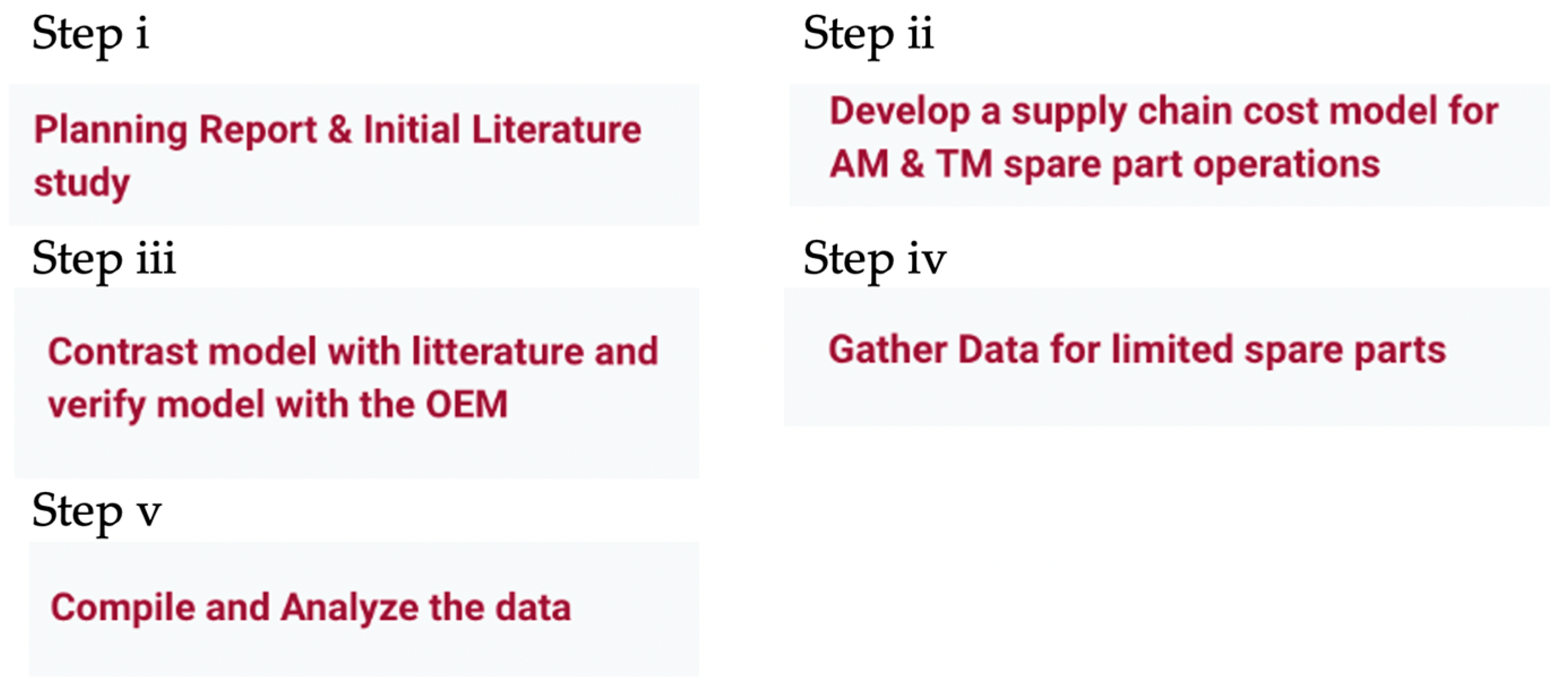
3.1. Case Study
- i.
- The planning report was created to align various stakeholders. In addition, an initial literature review of the current research streams and previous case studies of SPSC cost models was conducted. Cost models from prior research were used to lay the foundation of the cost model, with amendments during interviews. The supply chain cost models by Khajavi et al. [4], Li et al. [13] and Holmström et al. [27] were used as the basis of the model. Case studies were used to describe the warehousing costs.
- ii.
- An SPSC cost model for AM and TM spare part operations was developed. This was conducted by interviewing stakeholders at the OEM. From the interviews, a map of the supply chain value flows for TM was constructed. The TM SPSC value flow was then amended to resemble the AM production flow.
- iii.
- The created cost model was compared with the literature, and was verified with the OEM to resemble the actual SPSC and its inherent characteristics.
- iv.
- Fourteen spare parts for TM and AM were selected and the data was collected to calculate their supply chain costs. The selection of parts was carried out by assessing them from a financial and technical perspective. This was conducted by accessing databases, tools, and data sheets gathered from the interviewees. Interview and data gathering was with an AM supplier.
- v.
- After the calculation of the costs and comparison of different scenarios, analysis of the findings was performed.
3.2. Data Collection
3.3. Part Information and Pre-Screening Process
3.4. The OEM’s Spare Parts Supply Chain
- I
- In-house centralized SPSC
- II
- In-house decentralized SPSC
- III
- Outsourced centralized SPSC
- IV
- Outsourced decentralized SPSC
4. Results
4.1. AM and TM Cost Components of the OEM’s SPSC
4.1.1. Cost of Production
4.1.2. Cost of Inbound Transport
4.1.3. Cost of Warehousing
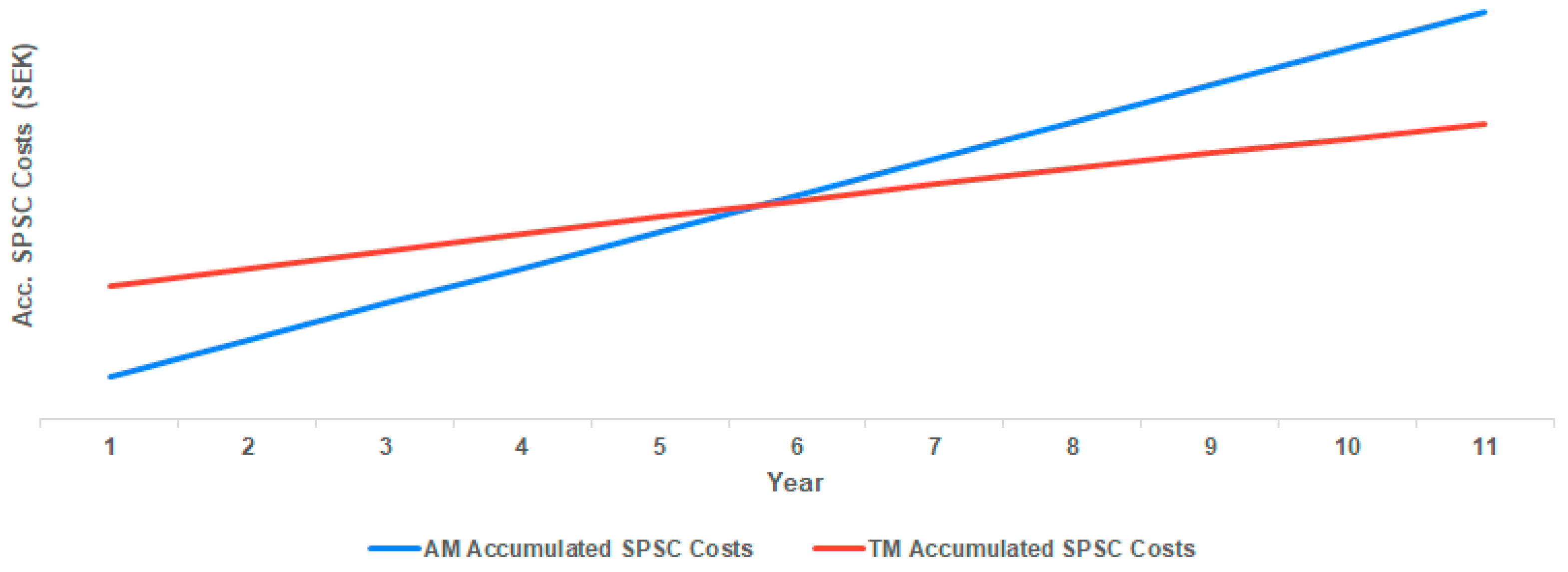
4.1.4. Inventory Control
Inventory Control for Traditional Manufacturing
- The Responsibility (Resp.) Year is set by the OEM internally and represents the planned final date of sales for a spare part.
- Max. value, the planning horizon cannot be longer than 15 years in the model. In reality, the OEM could provide spare parts for a longer time but are, according to regulations, only required to for 15 years after the end of production. This restriction was added to demarcate the model.
- SL < TSL, the year before the service level (SL) for TM falls below the target service level (TSL) as the TSL can be seen as a form of minimum safety stock level.
Inventory Control for Additive Manufacturing
4.1.5. Cost of Outbound Transport
4.1.6. Cost of Service
Cost of Vehicle off Road
- Offer a replacement truck if the truck is not repaired within the first four hours.
- If the OEM is not able to provide a replacement truck, the company is required to pay a VOR penalty fee. This penalty fee grows the longer the truck is out of use. Consequently, this makes the OEM keen on solving the VOR quickly which is carried out through a fast provision of spare parts.
Cost of Badwill
Cost of Lost Sales
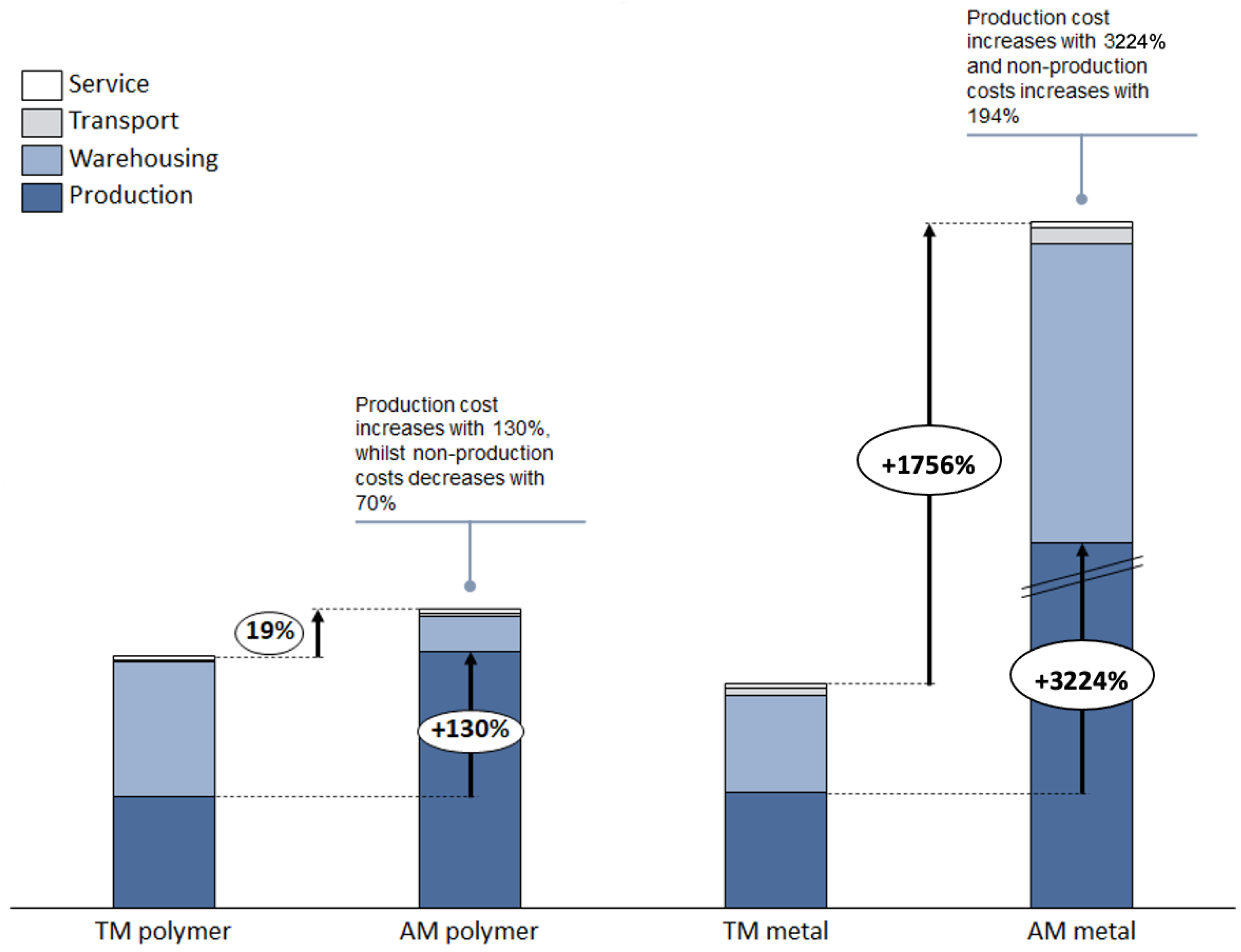
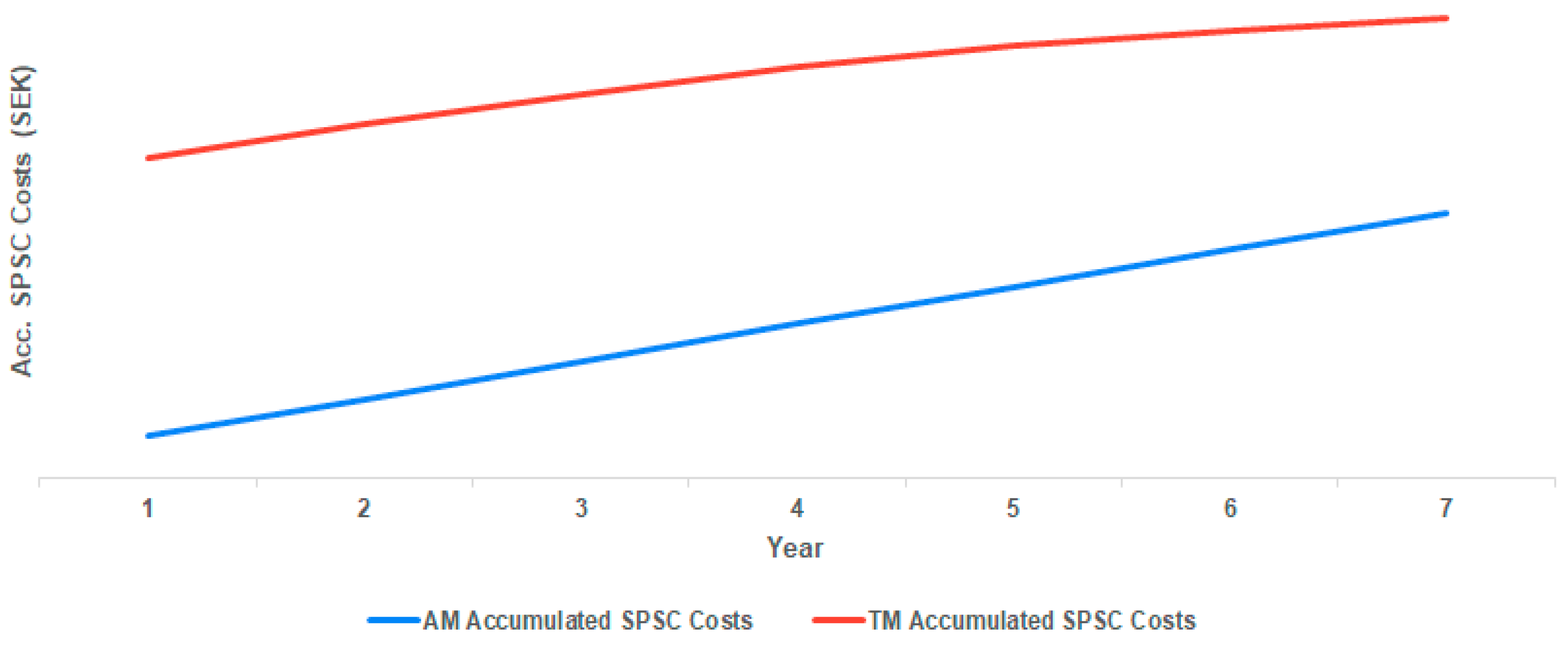
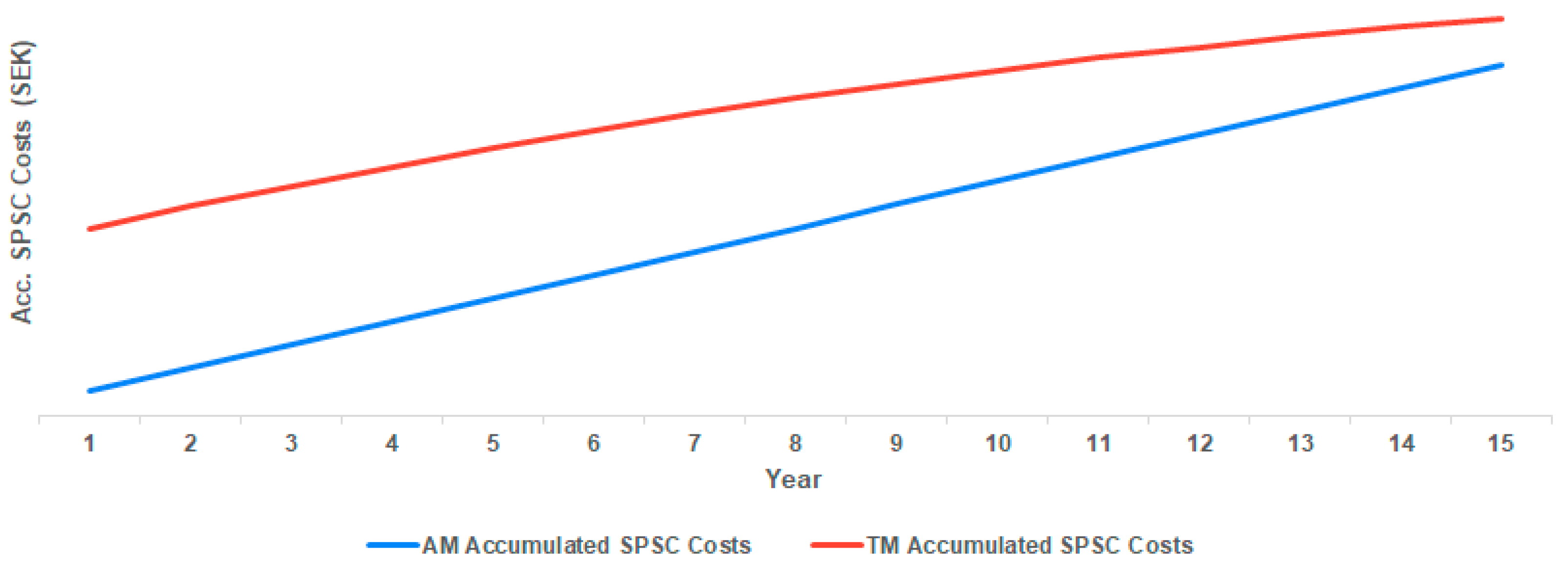
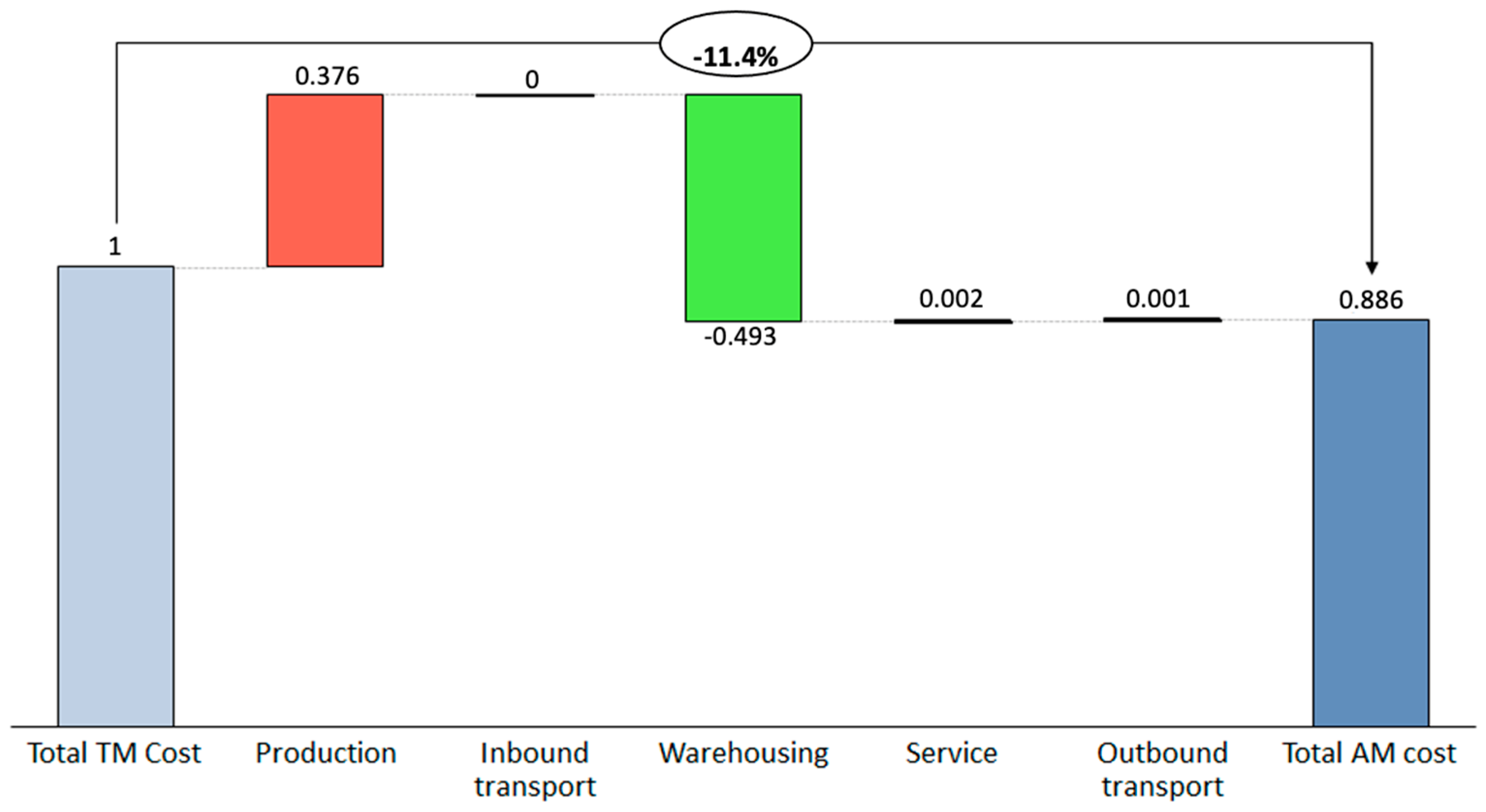
4.2. Average Total Cost of Spare Parts Supply Chain
- Polymer parts produced with TM
- Polymer parts produced with AM
- Metal parts produced with TM
- Metal parts produced with AM
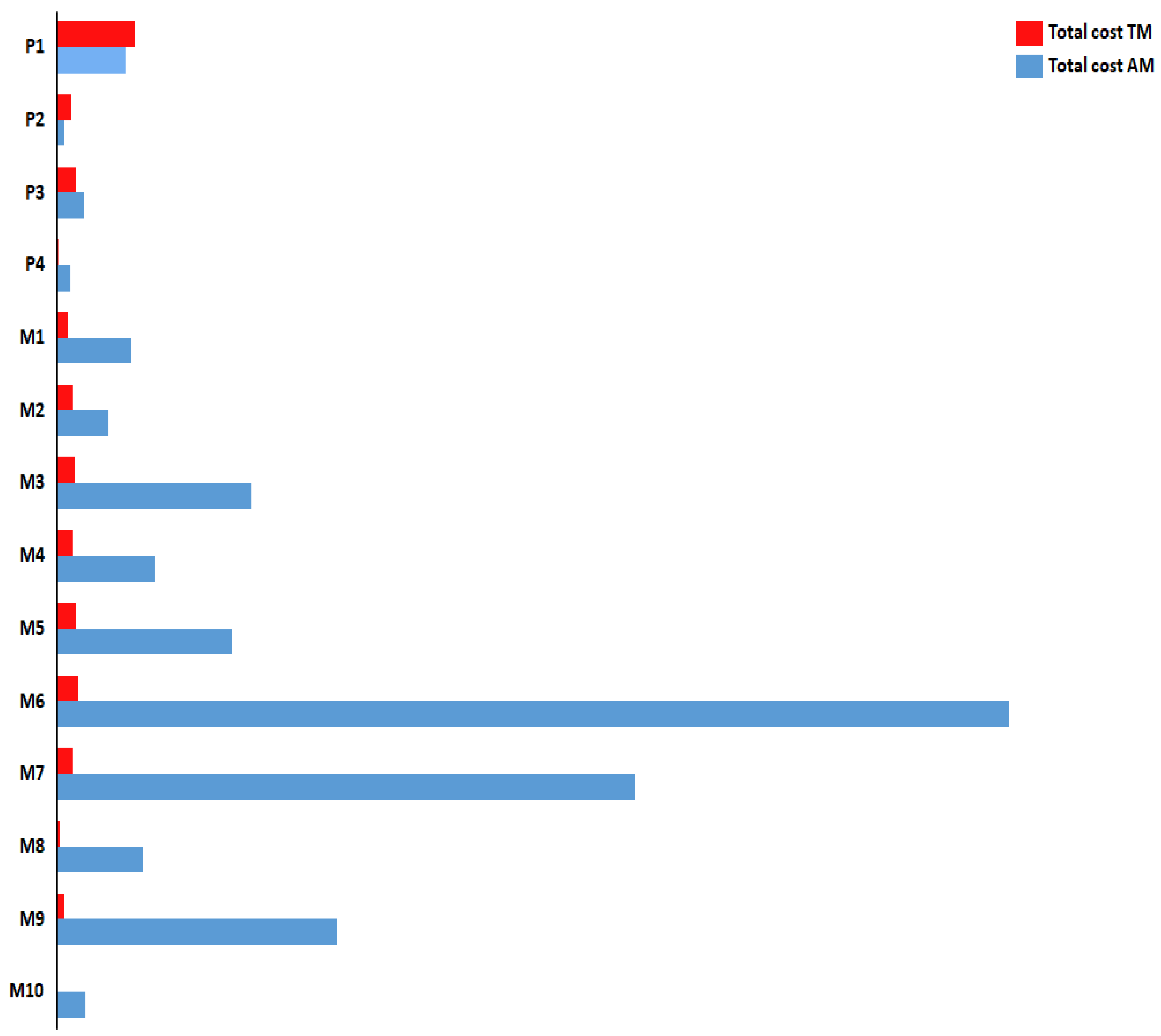
4.3. Total Cost Analysis of SPSC for Individual Parts
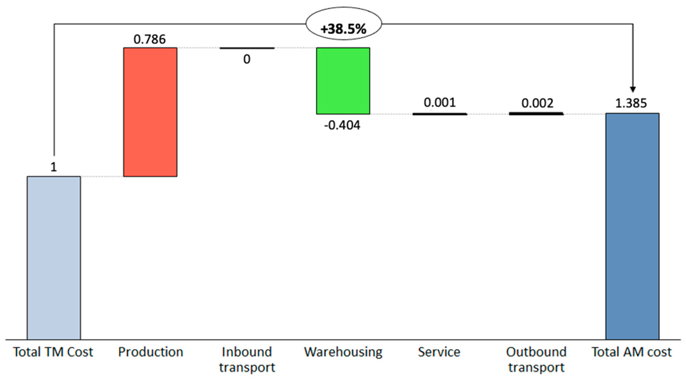
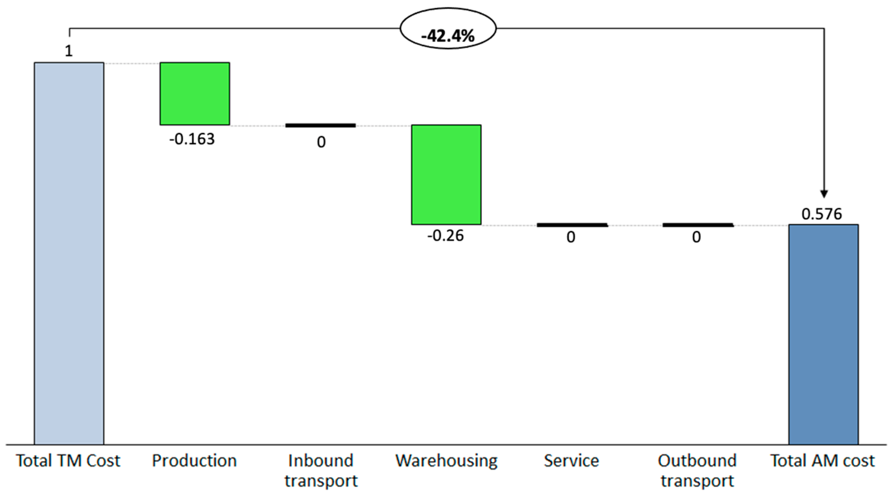
4.3.1. P3—A-Pillar
4.3.2. P2-Tappet
4.3.3. P1—Protecting Cover
5. Discussion
6. Conclusions
Author Contributions
Funding
Data Availability Statement
Conflicts of Interest
Appendix A
| Type of Database | Use in Model |
|---|---|
| Engineering database | Weight, material, dimensions, CAD-models |
| Warehouse Management System | Inventory, yearly demand, MOQ, standard price |
| Outbound transport database | Outbound transport cost |
| Inventory optimization tool | Cost of lost sales and badwill cost |
| After-sales-service software solution | Demand distribution |
| Inbound transport database | Inbound transport cost |
| Simulation Tool/Cost to serve | Warehousing costs |
| Database of operative operations | VOR |
| Supply and demand planning database. | Responsibility year |
Appendix B
| Filter Type | Condition | Motivation for Filtration |
|---|---|---|
| Article Price | >25 SEK | If the article price for TM was below 25 SEK, a business case for AM was deemed to be unfeasible, as AM is a significantly more expensive means of production. |
| Stock Value | >10,000 SEK | To find articles where the OEM could profit a significant amount. |
| Demand per year | >0; <40 pcs. | Less than 40 as a higher demand per year would likely benefit TM via economies of scale. Greater than 0 to remove outdated and non-active SKUs. |
| Current MOQ | LOQ = MOQ | To exclude cases where the MOQ has changed since the last shipment. In addition, to solidify the quantity ordered in LOQ was due to the suppliers MOQ-requirement. |
| LOQ-date older than 2018 | Older than 2018 | The demand data would have been inadequate for parts with a LOQ earlier than 2018. |
| SB higher than 0 | SB > 0 | The yearly demand data would have otherwise not been able to be computed. |
| Spare part being located in Europe CDC | - | The model developed in this thesis concerns Europe CDC. |
| Spare parts in specific business unit of OEM’s product portfolio | - | Request from stakeholders at OEM. |
| Weight restriction | Weight < 3000 g | Heavier parts lead to too high AM production prices. |
References
- de Souza, R.; Wee Kwan Tan, A.; Othman, H.; Garg, M. A Proposed Framework for Managing Service Parts in Automotive and Aerospace Industries. Benchmarking Int. J. 2011, 18, 769–782. [Google Scholar] [CrossRef]
- Cohen, M.A.; Agrawal, N.; Agrawal, V. Winning in the Aftermarket. Harv. Bus. Rev. 2006, 84, 129. [Google Scholar]
- Mellor, S.; Hao, L.; Zhang, D. Additive Manufacturing: A Framework for Implementation. Int. J. Prod. Econ. 2014, 149, 194–201. [Google Scholar] [CrossRef]
- Khajavi, S.H.; Partanen, J.; Holmström, J. Additive Manufacturing in the Spare Parts Supply Chain. Comput. Ind. 2014, 65, 50–63. [Google Scholar] [CrossRef]
- Gibson, I.; Rosen, D.W.; Stucker, B. Additive Manufacturing Technologies, 17th ed.; Springer: New York, NY, USA, 2014. [Google Scholar]
- Rogers, H.; Baricz, N.; Pawar, K.S. 3D Printing Services: Classification, Supply Chain Implications and Research Agenda. Int. J. Phys. Distrib. Logist. Manag. 2016, 46, 886–907. [Google Scholar] [CrossRef]
- Khorasani, M.; Ghasemi, A.; Rolfe, B.; Gibson, I. Additive Manufacturing a Powerful Tool for the Aerospace Industry. Rapid Prototyp. J. 2022, 28, 87–100. [Google Scholar] [CrossRef]
- Pettersson, A.I.; Segerstedt, A. Measuring Supply Chain Cost. Int. J. Prod. Econ. 2013, 143, 357–363. [Google Scholar] [CrossRef]
- Attaran, M. Additive Manufacturing: The Most Promising Technology to Alter the Supply Chain and Logistics. J. Serv. Sci. Manag. 2017, 10, 189–206. [Google Scholar] [CrossRef]
- Bozarth, C.C.; Handfield, R.B. Introduction to Operations and Supply Chain Management; Pearson: London, UK, 2016. [Google Scholar]
- Van Houtum, G.; Kranenburg, B. Spare Parts Inventory Control under System Availability Constraints, 127th ed.; Springer: Berlin/Heidelberg, Germany, 2015; ISBN 978-1-4899-7609-3. [Google Scholar]
- Huiskonen, J. Maintenance Spare Parts Logistics: Special Characteristics and Strategic Choices. Int. J. Prod. Econ. 2001, 71, 125–133. [Google Scholar] [CrossRef]
- Li, Y.; Jia, G.; Cheng, Y.; Hu, Y. Additive Manufacturing Technology in Spare Parts Supply Chain: A Comparative Study. Int. J. Prod. Res. 2017, 55, 1498–1515. [Google Scholar] [CrossRef]
- Markillie, P. The Economist; The Economist group: London, UK, 2012; pp. 3–12. [Google Scholar]
- Freichel, S. The Sum of the Parts. Supply Chain. Eur. 2010, 19, 38–39. [Google Scholar]
- ACEA, Legacy Spare Parts Supporting Document. European Automobile Manufacturers Association. Available online: https://ec.europa.eu/DocsRoom/documents/10705/attachments/1/translations/en/renditions/native (accessed on 13 December 2020).
- Dombrowski, U.; Engel, C.; Schulze, S. Scenario Management for Sustainable Strategy Development in the Automotive Aftermarket. In Functional Thinking for Value Creation; Springer: Berlin/Heidelberg, Germany, 2011; pp. 285–290. [Google Scholar]
- Thomopoulus, N. Elements of Manufacturing, Distribution and Logistics; Springer: Berlin/Heidelberg, Germany, 2016. [Google Scholar]
- Schönsleben, P. Integral Logistics Management—Operations Management and Supply Chain Management Within and Across Companies; CRC Press: Boca Raton, FL, USA, 2016. [Google Scholar]
- La Londe, B.J.; Lambert, D.M. Inventory Carrying Costs: Significance, Components, Means, Functions. Int. J. Phys. Distrib. 1975, 6, 51–63. [Google Scholar] [CrossRef]
- Park, Y.W.; Klabjan, D. Lot Sizing with Minimum Order Quantity. Discret. Appl. Math. 2015, 181, 235–254. [Google Scholar] [CrossRef]
- Rengier, F.; Mehndiratta, A.; von Tengg-Kobligk, H.; Zechmann, C.M.; Unterhinninghofen, R.; Kauczor, H.-U.; Giesel, F.L. 3D Printing Based on Imaging Data: Review of Medical Applications. Int. J. Comput. Assist. Radiol. Surg. 2010, 5, 335–341. [Google Scholar] [CrossRef]
- Ukobitz, D.; Faullant, R. Leveraging 3D Printing Technologies: The Case of Mexico’s Footwear Industry. Res. Manag. 2021, 64, 20–30. [Google Scholar] [CrossRef]
- PwC 3D Printing: A Potential Game Changer for Aerospace and Defense. Available online: www.pwc.com/us/en/industrial-products/publications/assets/pwc-gaining-altitude-issue-7-%0A3d-printing.pdf (accessed on 15 December 2020).
- Eyers, D. Flexibility Strategies for 3DP. In Managing 3D Printing; Springer International Publishing: Cham, Switzerland, 2020; pp. 77–96. [Google Scholar]
- Wohlers, T.; Gornet, T. History of Additive Manufacturing; Wohlers Associates, Inc.: Fort Collins, CO, USA, 2014. [Google Scholar]
- Holmström, J.; Partanen, J.; Tuomi, J.; Walter, M. Rapid Manufacturing in the Spare Parts Supply Chain. J. Manuf. Technol. Manag. 2010, 21, 687–697. [Google Scholar] [CrossRef]
- Holmström, J.; Gutowski, T. Additive Manufacturing in Operations and Supply Chain Management: No Sustainability Benefit or Virtuous Knock-On Opportunities? J. Ind. Ecol. 2017, 21, S21–S24. [Google Scholar] [CrossRef]
- Heinen, J.J.; Hoberg, K. Assessing the Potential of Additive Manufacturing for the Provision of Spare Parts. J. Oper. Manag. 2019, 65, 810–826. [Google Scholar] [CrossRef]
- Liu, P.; Huang, S.H.; Mokasdar, A.; Zhou, H.; Hou, L. The Impact of Additive Manufacturing in the Aircraft Spare Parts Supply Chain: Supply Chain Operation Reference (Scor) Model Based Analysis. Prod. Plan. Control 2014, 25, 1169–1181. [Google Scholar] [CrossRef]
- Chan, H.K.; Griffin, J.; Lim, J.J.; Zeng, F.; Chiu, A.S.F. The Impact of 3D Printing Technology on the Supply Chain: Manufacturing and Legal Perspectives. Int. J. Prod. Econ. 2018, 205, 156–162. [Google Scholar] [CrossRef]
- Thomas-Seale, L.E.J.; Kirkman-Brown, J.C.; Attallah, M.M.; Espino, D.M.; Shepherd, D.E.T. The Barriers to the Progression of Additive Manufacture: Perspectives from UK Industry. Int. J. Prod. Econ. 2018, 198, 104–118. [Google Scholar] [CrossRef]
- Salmi, M.; Partanen, J.; Tuomi, J.; Chekurov, S.; Björkstrand, R.; Huotilainen, E.; Kukko, K.; Kretzschmar, N.; Akmal, J.; Jalava, K.; et al. Digital Spare Parts; Aalto University and VTT Technical Research Centre of Finland: Espoo, Finland, 2018; ISBN 978-952-60-3746-2. [Google Scholar]
- Degraeve, Z.; Labro, E.; Roodhooft, F. An Evaluation of Vendor Selection Models from a Total Cost of Ownership Perspective. Eur. J. Oper. Res. 2000, 125, 34–58. [Google Scholar] [CrossRef]
- Van Weele, A. Purchasing and Supply Chain Management (PSCM), 7th ed.; Cengage: Boston, MA, USA, 2018. [Google Scholar]
- Holmström, J.; Holweg, M.; Khajavi, S.H.; Partanen, J. The Direct Digital Manufacturing (r)Evolution: Definition of a Research Agenda. Oper. Manag. Res. 2016, 9, 1–10. [Google Scholar] [CrossRef]
- Khajavi, S.H.; Holmström, J.; Partanen, J. Additive Manufacturing in the Spare Parts Supply Chain: Hub Configuration and Technology Maturity. Rapid Prototyp. J. 2018, 24, 1178–1192. [Google Scholar] [CrossRef]
- Martynovich, M. General Purpose Technology Diffusion and Labour Market Dynamics: A Spatio-Temporal Perspective; Lund University: Lund, Sweden, 2016. [Google Scholar]
- Holmström, J.; Partanen, J. Digital Manufacturing-Driven Transformations of Service Supply Chains for Complex Products. Supply Chain Manag. Int. J. 2014, 19, 421–430. [Google Scholar] [CrossRef]
- Thomas, D. Costs, Benefits, and Adoption of Additive Manufacturing: A Supply Chain Perspective. Int. J. Adv. Manuf. Technol. 2016, 85, 1857–1876. [Google Scholar] [CrossRef]
- Alogla, A.A.; Baumers, M.; Tuck, C.; Elmadih, W. The Impact of Additive Manufacturing on the Flexibility of a Manufacturing Supply Chain. Appl. Sci. 2021, 11, 3707. [Google Scholar] [CrossRef]
- Knofius, N.; van der Heijden, M.C.; Zijm, W.H.M. Selecting Parts for Additive Manufacturing in Service Logistics. J. Manuf. Technol. Manag. 2016, 27, 915–931. [Google Scholar] [CrossRef]
- Atzeni, E.; Salmi, A. Economics of Additive Manufacturing for End-Usable Metal Parts. Int. J. Adv. Manuf. Technol. 2012, 62, 1147–1155. [Google Scholar] [CrossRef]
- Hopkinson, N.; Dicknes, P. Analysis of Rapid Manufacturing—Using Layer Manufacturing Processes for Production. Proc. Inst. Mech. Eng. Part C J. Mech. Eng. Sci. 2003, 217, 31–39. [Google Scholar] [CrossRef]
- Lindemann, C.; Jahnke, U.; Moi, M.; Koch, R. Analyzing Product Life Cycle Costs for a Better Understanding of Cost Drivers in Additive Manufacturing. In Proceedings of the 23th Annual International Solid Freeform Fabrication Symposium—An Additive Manufacturing Conference, Austin, TX, USA, 6–8 August 2012. [Google Scholar]
- Ruffo, M.; Tuck, C.; Hague, R. Cost Estimation for Rapid Manufacturing—Laser Sintering Production for Low to Medium Volumes. Proc. Inst. Mech. Eng. Part B J. Eng. Manuf. 2006, 220, 1417–1427. [Google Scholar] [CrossRef]
- Thomas, D.S.; Gilbert, S.W. NIST Special Publication 1176; National Institute of Standards and Technology: Gaithersburg, MD, USA, 2014.
- Meboldt, M.; Klahn, C. Industrializing Additive Manufacturing. In Proceedings of the Additive Manufacturing in Products and Applications-AMPA2017; Springer: Berlin/Heidelberg, Germany, 2017; pp. 226–235. [Google Scholar]
- Knofius, N.; van der Heijden, M.C.; Sleptchenko, A.; Zijm, W.H.M. Improving Effectiveness of Spare Parts Supply by Additive Manufacturing as Dual Sourcing Option. OR Spectr. 2021, 43, 189–221. [Google Scholar] [CrossRef]
- Yin, R.K. Applications of Case Study Research; Sage: New York, NY, USA, 2011. [Google Scholar]
- Bryman, A.; Bell, E. Business Research Methods, 4th ed.; Bell & Bain Ltd.: Glasgow, UK, 2016; ISBN 978-0-19-958340-9. [Google Scholar]
- Brooks, H.; Molony, S. Design and Evaluation of Additively Manufactured Parts with Three Dimensional Continuous Fibre Reinforcement. Mater. Des. 2016, 90, 276–283. [Google Scholar] [CrossRef]
- Khajavi, S.H.; Partanen, J.; Holmström, J.; Tuomi, J. Risk Reduction in New Product Launch: A Hybrid Approach Combining Direct Digital and Tool-Based Manufacturing. Comput. Ind. 2015, 74, 29–42. [Google Scholar] [CrossRef]


| Item No. | Name | Material | Weight [Grams] | Volume [cm3] | Annual Demand | MOQ |
|---|---|---|---|---|---|---|
| P1 | PROTECTING COVER | Polymer | 150 | 92.73 | 23 | 500 |
| P2 | TAPPET | Polymer | 407 | 433.26 | 6 | 50 |
| P3 | A-PILLAR | Polymer | 193 | 157.13 | 6 | 243 |
| P4 | SWITCH PANEL | Polymer | 52 | 44.97 | 29 | 192 |
| M1 | SPACER | Aluminum | 410 | 155.07 | 2 | 95 |
| M2 | HUB | Steel | 1310 | 164.66 | 3 | 100 |
| M3 | BRACKET | Steel | 2015 | 264.4 | 3 | 60 |
| M4 | INTERMEDIATE SECTION | Graphite Iron | 696 | 96.09 | 6 | 100 |
| M5 | HOLLOW DRIFT | Steel | 1600 | 198.22 | 4 | 50 |
| M6 | CUP | Steel | 2900 | 366.01 | 16 | 150 |
| M7 | BRACKET | Graphite Iron | 1650 | 175.04 | 17 | 100 |
| M8 | BRACKET | Steel | 117 | 15 | 32 | 170 |
| M9 | ATTACHING PLATE | Graphite Iron | 1868 | 265.12 | 5 | 54 |
| M10 | CONNECTOR | Aluminum | 81 | 28.45 | 9 | 60 |
| Cost Sub-Component | Factor and Cost Driver | Description |
|---|---|---|
| Goods in | # of SEK (Swedish krona) × # of received lines * during the year. [SEK/received delivery] | Cost for handling and transporting goods from the truck to the location inside the warehouse, e.g., labor cost and forklift cost. |
| Capital costs | # % of the stock value at the beginning of the year. Percentage value based on Internal Rate of Return. [SEK/inventory value ***] | Alternative cost for the capital not being invested in other lucrative businesses and thereby generate positive cash flow to the OEM. |
| Packaging | # % of the annual turnover. [SEK/turnover value ****] | Cost for packing the goods before sending them to the dealer. |
| Goods out | # of SEK × # of order lines ** during the year. [SEK/order line] | Cost for handling and transporting goods from the location inside the warehouse to the truck, e.g., labor cost and forklift cost. |
| Procurement | # of SEK × # of received lines during the year. [SEK/received delivery] | Personal cost for maintaining the relationship with the supplier. |
| Warehouse overhead cost | # of % of annual turnover. [SEK/turnover value] | Salaries for managers running the warehouse. |
| Order office | # of SEK × # of order lines during the year. [SEK/order line] | Personal cost for administering the orders made by the dealers. |
| Warehouse building | # of SEK × average weight stored in the warehouse during the year. [SEK/Kg] | Cost for storing goods in the warehouse. |
| Development | # of % of annual turnover. [SEK/turnover value] | Personal cost for developing the service market logistics. |
| Area | TM | AM |
|---|---|---|
| Replenishment | One received shipment for the whole planning horizon | Annual Replenishments |
| Safety stock | Safety stock equivalent to where service level is equal to target service level. | Safety stock set to one pc. |
| Service level | Probability for average inventory level to be greater than average yearly demand, changing between years. | SERV1, constant for all years |
| Average inventory level | (Inventory level at the beginning of the year + inventory of the next year)/2 | Safety stock + (order quantity)/2 |
| Item No. | Planning Horizon Years | Reason for Planning Horizon End |
|---|---|---|
| P1 | 15 | Max. value |
| P2 | 7 | SL < TSL |
| P3 | 11 | Resp. |
| P4 | 5 | S L< TSL |
| M1 | 14 | Resp. |
| M2 | 4 | Resp. |
| M3 | 9 | Resp. |
| M4 | 6 | Resp. |
| M5 | 7 | Resp. |
| M6 | 7 | Resp. |
| M7 | 4 | SL < TSL |
| M8 | 4 | SL < TSL |
| M9 | 9 | SL < TSL |
| M10 | 5 | SL < TSL |
| Item No. | Material | AM-Technology |
|---|---|---|
| P1 | Polymer: Polyurethan | Indirect AM * |
| P2 | Polymer: Thermoplastic | FDM |
| P3 | Polymer: PA12 | SLS |
| P4 | Polymer: Polyurethan | Indirect AM * |
| M1 | Metal: AlSiMg10 | SLM |
| M2 | Metal: SS316L | SLM |
| M3 | Metal: SS316L | SLM |
| M4 | Metal: SS316L | SLM |
| M5 | Metal: SS316L | SLM |
| M6 | Metal: SS316L | SLM |
| M7 | Metal: SS316L | SLM |
| M8 | Metal: SS316L | SLM |
| M9 | Metal: SS316L | SLM |
| M10 | Metal: AlSiMg10 | SLM |
Disclaimer/Publisher’s Note: The statements, opinions and data contained in all publications are solely those of the individual author(s) and contributor(s) and not of MDPI and/or the editor(s). MDPI and/or the editor(s) disclaim responsibility for any injury to people or property resulting from any ideas, methods, instructions or products referred to in the content. |
© 2022 by the authors. Licensee MDPI, Basel, Switzerland. This article is an open access article distributed under the terms and conditions of the Creative Commons Attribution (CC BY) license (https://creativecommons.org/licenses/by/4.0/).
Share and Cite
Ahlsell, L.; Jalal, D.; Khajavi, S.H.; Jonsson, P.; Holmström, J. Additive Manufacturing of Slow-Moving Automotive Spare Parts: A Supply Chain Cost Assessment. J. Manuf. Mater. Process. 2023, 7, 8. https://doi.org/10.3390/jmmp7010008
Ahlsell L, Jalal D, Khajavi SH, Jonsson P, Holmström J. Additive Manufacturing of Slow-Moving Automotive Spare Parts: A Supply Chain Cost Assessment. Journal of Manufacturing and Materials Processing. 2023; 7(1):8. https://doi.org/10.3390/jmmp7010008
Chicago/Turabian StyleAhlsell, Levin, Didar Jalal, Siavash H. Khajavi, Patrik Jonsson, and Jan Holmström. 2023. "Additive Manufacturing of Slow-Moving Automotive Spare Parts: A Supply Chain Cost Assessment" Journal of Manufacturing and Materials Processing 7, no. 1: 8. https://doi.org/10.3390/jmmp7010008
APA StyleAhlsell, L., Jalal, D., Khajavi, S. H., Jonsson, P., & Holmström, J. (2023). Additive Manufacturing of Slow-Moving Automotive Spare Parts: A Supply Chain Cost Assessment. Journal of Manufacturing and Materials Processing, 7(1), 8. https://doi.org/10.3390/jmmp7010008