Calibrated Probabilistic Forecasting and Measured Discharge Physics for Deliverable Electric Vehicle Flexibility

Abstract

Electric vehicle (EV) charging has a large, spatially clustered, schedulable load whose vehicle-to-grid flexibility can be sold back to the power system. That flexibility has grid value only when the committed quantity can be reliably delivered under uncertainty. Open forecasting benchmarks operators rely on report-only point predictions. The dispatch models that turn forecasts into firm commitments assume a constant round-trip efficiency, so the committed flexibility is systematically over-scheduled. This study contributes two complementary modules, validated separately on public data. The first is a calibrated probabilistic charging forecaster that provides, to our knowledge, the first prediction intervals with reported empirical coverage on the UrbanEV benchmark. It is a gradient-boosted quantile-regression model that combines each zone’s own-history lags with adjacency-weighted neighbor-mean features and exogenous price and calendar inputs. It is calibrated by conformalized quantile regression and scored over thirty zones across a 120-day hourly window. The second is a deliverable-flexibility envelope whose returnable-energy bounds are set by measured, state-of-charge- and rate-dependent vehicle-to-grid (V2G) discharge efficiency rather than a constant round-trip number. These bounds are fit to the measured discharge traces of three V2G-capable vehicles in the Esser bidirectional-charging dataset. Chosen as a lightweight, reproducible baseline, the forecaster keeps its prediction intervals within a five-percentage-point coverage tolerance at both the 80% and 90% nominal levels. Measured coverage is 0.823 and 0.911. It also improves on the continuous ranked probability score of its conformalized-point counterpart at matched point accuracy. This calibration holds across the hyperparameter neighborhood and under data deficiency. On the delivery side, a leave-one-vehicle oracle shows the efficiency-aware envelope short-delivers less than the constant-average-efficiency aggregator on held-out vehicles. Its residual shortfall is 1.21% against the aggregator’s 2.03% at the conservative operating point. The margin widens as commitments grow more aggressive and discharges reach the lowest states of charge. Each of these two measured properties, calibrated demand-side uncertainty and state-dependent discharge physics, imposes a material, separately validated constraint on how much contracted EV flexibility can be delivered, a constraint the point-forecasting frontier leaves unaddressed.

1. Introduction

Decarbonizing electricity supply has shifted the operating problem of power systems. The task is no longer to balance a predictable load against dispatchable generation. It is to balance a variable, weather-driven generation mix against a load that must itself become flexible. Electric vehicles sit at the center of this shift. A charging EV draws several kilowatts to tens of kilowatts, and fleets cluster in time around commuting and overnight patterns. The energy a vehicle needs over a session is bounded while its moment-to-moment power is negotiable. A bidirectional, V2G-capable vehicle extends this further still. It can absorb surplus generation, return energy during scarcity, and stand in for fast-responding reserve. Aggregated across a city, this is a controllable resource comparable in magnitude to conventional balancing assets. Operators and aggregators increasingly treat it as such when they contract day-ahead energy shifting and ancillary services.

There is a large economic stake in getting this right. Flexibility that is contracted but not delivered is penalized through imbalance settlement and degraded ancillary-service performance scores. Repeated non-delivery erodes the qualification that lets a resource participate at all. The value of EV flexibility therefore depends not on the capacity a fleet nominally possesses, but on how much it can commit and reliably honor under uncertainty. This makes the EV a representative and high-consequence instance of a broader class of demand-side resources. Their grid value is realized only when forecasts of their behavior and models of their physical limits support a firm promise.

Turning aggregate EV charging into deliverable flexibility involves two coupled requirements, and a commitment is firm only when both are met. The first link is the forecast. An operator deciding how much flexibility to offer for the upcoming hours must know the expected charging demand of each zone. It must also know the distribution of that demand. The offer is a quantity that must hold with a stated probability. The second link is the physics of delivery. When a V2G commitment is dispatched, the energy that actually crosses the meter is governed by a discharge efficiency. That efficiency depends on the battery’s state of charge and on the rate of power flow. That efficiency varies far more across operating states than a single round-trip number admits. A plan that ignores either link will look feasible on paper and fall short in operation.

This study addresses each of these two requirements. On the forecasting side it asks how to obtain a calibrated, distributional charging forecast whose coverage is controlled on the observable charging-demand target. On the delivery side it asks how to build a flexibility region whose returnable-energy bounds follow measured rather than assumed efficiency. A third aim is to quantify the delivery shortfall a practitioner incurs by retaining the conventional constant-efficiency assumption. The two questions share a failure mode. A forecast without calibrated uncertainty and a dispatch plan without delivery physics both push toward over-commitment, the failure that the penalty structure penalizes most heavily. What the existing literature offers each question, and where it stops short, sets up the two gaps this study fills.

On the forecasting side, the dominant accuracy work treats the spatial structure explicitly, because zone-level charging demand is spatially clustered and the coupling between zones is real. The graph-neural lineage opens with DCRNN [1], which casts spatial dependence as a diffusion process along a fixed sensor graph. STGCN [2] interleaves gated temporal convolutions with graph convolutions. Both show that a predefined adjacency between locations carries predictive signal that purely temporal models discard. The lineage continues through ASTGCN [3], which weights the graph and the history with spatial and temporal attention so the spatial coupling can vary with context. Graph WaveNet [4] learns a self-adaptive adjacency directly from data alongside dilated causal convolutions. AGCRN [5] pushes this furthest, generating the graph and node-specific parameters adaptively so no predefined adjacency is needed. MTGNN [6] learns a graph for generic multivariate series and propagates over it. Exploiting an inter-zone adjacency, whether fixed or learned, improves accuracy over zone-by-zone time-series models. A time-varying adjacency that strengthens at commute peaks and relaxes overnight could in principle add further signal.

Alongside spatial structure, the transformer family demonstrates that exogenous conditioning on calendar and price signals improves charging-demand forecasts. PatchTST [7] segments each series into subseries patches that serve as attention tokens, lengthening the usable context at tractable cost. TimesNet [8] folds the one-dimensional series into two-dimensional tensors along its dominant periods so that intra- and inter-period variation are modeled jointly. Neither, however, carries an explicit pathway for exogenous inputs. iTransformer [9] inverts the usual layout, embedding each variate as a token so that attention runs across variables rather than across time. That cross-variable attention is the mechanism by which an exogenous price or calendar series informs the target. TimeXer [10] makes the pathway explicit, attending over patch-level tokens of the endogenous series while admitting exogenous series as variate-level tokens through cross-attention. It is the reported point-accuracy leader on UrbanEV [11], which sets the accuracy bar on this benchmark. EV-specific designs add domain structure on top of these generic backbones. The physics-informed graph learning model of Kuang et al. [12] embeds a price-elasticity relation into a graph network, evidence that EV charging carries exploitable price structure. There, the price structure is built into the network as an explicit elasticity law rather than admitted as a generic exogenous input. The adaptive spatio-temporal graph recurrent network of Wang et al. [13] learns a time-varying inter-zone graph for short-term EV charging demand. It is the closest recent EV forecaster on the same point-forecasting objective and the most direct point-accuracy reference for short-term zone-level charging demand. Two ingredients therefore recur across this line of work. The inter-zone adjacency is a useful spatial signal, and exogenous price and calendar conditioning matters. In each of these designs, both ingredients live inside an expressive learned architecture that emits point forecasts rather than the calibrated distribution a commitment must be bid against.

Accuracy alone, however, does not make a forecast biddable. A central finding from the probabilistic-forecasting literature is that point accuracy and calibration are different objectives that must be measured separately. DeepAR [14] trains an autoregressive recurrent network jointly across many related series and emits a parametric predictive distribution for each. It shows that distributional output can be learned directly rather than appended to a point model afterward. DiffPLF [15] carries the distributional objective to EV charging load specifically, generating the predictive distribution by conditional denoising diffusion. Both are single-site rather than spatiotemporal designs. The coherent hierarchical model of Zheng et al. [16] adds a structural property instead. Its probabilistic charging-demand forecasts aggregate consistently, so the distributional statements at different levels of the hierarchy cannot contradict one another. That hierarchy, however, is fixed in advance. None of these report coverage on UrbanEV. The reliability of an interval is read from the proportion-in-the-interval (PICP) against nominal. The normalized interval width guards against the trivial fix of widening intervals until coverage is met. The proper scoring rules, the continuous ranked probability score and the pinball loss reward distributions that are at once well-located and sharp [17]. Together, these metrics are what make a calibration claim falsifiable in the first place.

On the delivery side, literature on the aggregate-feasible-region supplies the geometry but not the physics. Minkowski-sum and polymatroid constructions and maximum-volume inner approximations [18] describe the set of fleet power trajectories a controller can realize. Their real-time coordination across a distributed charger population is itself a control problem [19]. The inner-approximation idea, certifying a set of which every point is feasible, is exactly the guarantee a bankable commitment needs. The unexamined assumption in this body of work is that the conversion between grid energy and stored energy is lossless or governed by a single constant efficiency. Whether that assumption is physically warranted is a question the geometry literature does not itself examine. Conversion efficiency may instead depend on state of charge and power strongly enough to invalidate a single constant. That this dependence is real, and not an artifact of any one dataset, is what independent cell-level work establishes. The experimental study of Su et al. [20] charges lithium-ion cells under a range of charging stresses. It shows that the charging energy efficiency is not a fixed coefficient but shifts systematically with rate and operating condition. This is the rate-dependence the discharge side mirrors. The mechanistic study of Cai et al. [21] traces coulombic loss to its electrochemical origin and shows how the loss varies across operating regimes rather than holding at a single value. This is why a constant efficiency mis-states the energy returned at the deep and high-rate states a V2G dispatch reaches. Together they confirm that this dependence is a property of the chemistry. A measured efficiency band rather than a scalar is therefore the physically faithful object to constrain the feasible region with.

What neither domain literature supplies on its own, two methods imported from outside EV forecasting do. The first is split conformal prediction and its quantile-regression form, conformalized quantile regression [22]. CQR takes a model that already emits conditional quantiles. It measures the conformity error on a held-out calibration block as the signed distance by which the truth falls outside the predicted band. It then shifts the band by the empirical quantile of that error. The result is finite-sample marginal coverage under exchangeability, achieved post hoc on top of any quantile model at the cost of a single scalar correction per nominal level. No retraining is needed, and no point accuracy is traded away. The group-conditional, or Mondrian, variant [23] computes the calibration correction within strata rather than over the pooled scores. The validity statement then holds per group instead of only marginally. Sousa et al. [24] carry that machinery to multi-step time-series forecasting, where the error distribution shifts with lead time and the forecast horizon becomes the natural stratum. The horizon-stratified correction thus stands as a stricter, per-lead-time alternative to a single pooled correction. Conformal prediction is field-agnostic by construction, making no assumption about the forecaster that produced the quantiles. It therefore transfers cleanly from distribution-free regression to short-term forecasting tasks such as solar power [25] and to spatiotemporal charging demand. Its finite-sample coverage does carry one condition. The calibration target must be observed and exchangeable with the test target. The guarantee therefore attaches to the metered charging demand, since the delivered-energy quantity is never observed under that same exchangeability.

A second transferable tool, drawn from the same risk-sizing literature and not evaluated in this study, is the risk measure conditional value-at-risk and its linear-programming reformulation [26]. Sizing a commitment under uncertain delivery is a decision under a heavy-tailed loss, and the Rockafellar–Uryasev result expresses a mean-minus-CVaR objective as a linear program over scenarios. That formulation would keep commitment sizing convex and let one scenario set carry both forecast and delivery uncertainty. Such a program would consume calibrated coverage on an observable target together with a measured-physics delivery envelope. Assembling those two inputs into a single commitment-sizing layer remains unaddressed in the EV-flexibility setting.

Assembled this way, the literature stops two gaps short of a deliverable commitment, and they sit precisely at the two links identified above. The first follows directly from the accuracy line. The dominant open EV forecasting benchmark and its top-performing model report point accuracy only, as root-mean-square and absolute error, with no quantiles and no coverage. An operator who adopts the state of the art therefore inherits a best guess but no calibrated distribution to bid against. Calibrated coverage has not been reported on the standard multi-zone EV benchmark at all, so the intersection of calibrated uncertainty and that benchmark is unoccupied. An offer derived from a point forecast therefore has no defensible probability attached, the property an ancillary-service or imbalance-settled commitment requires.

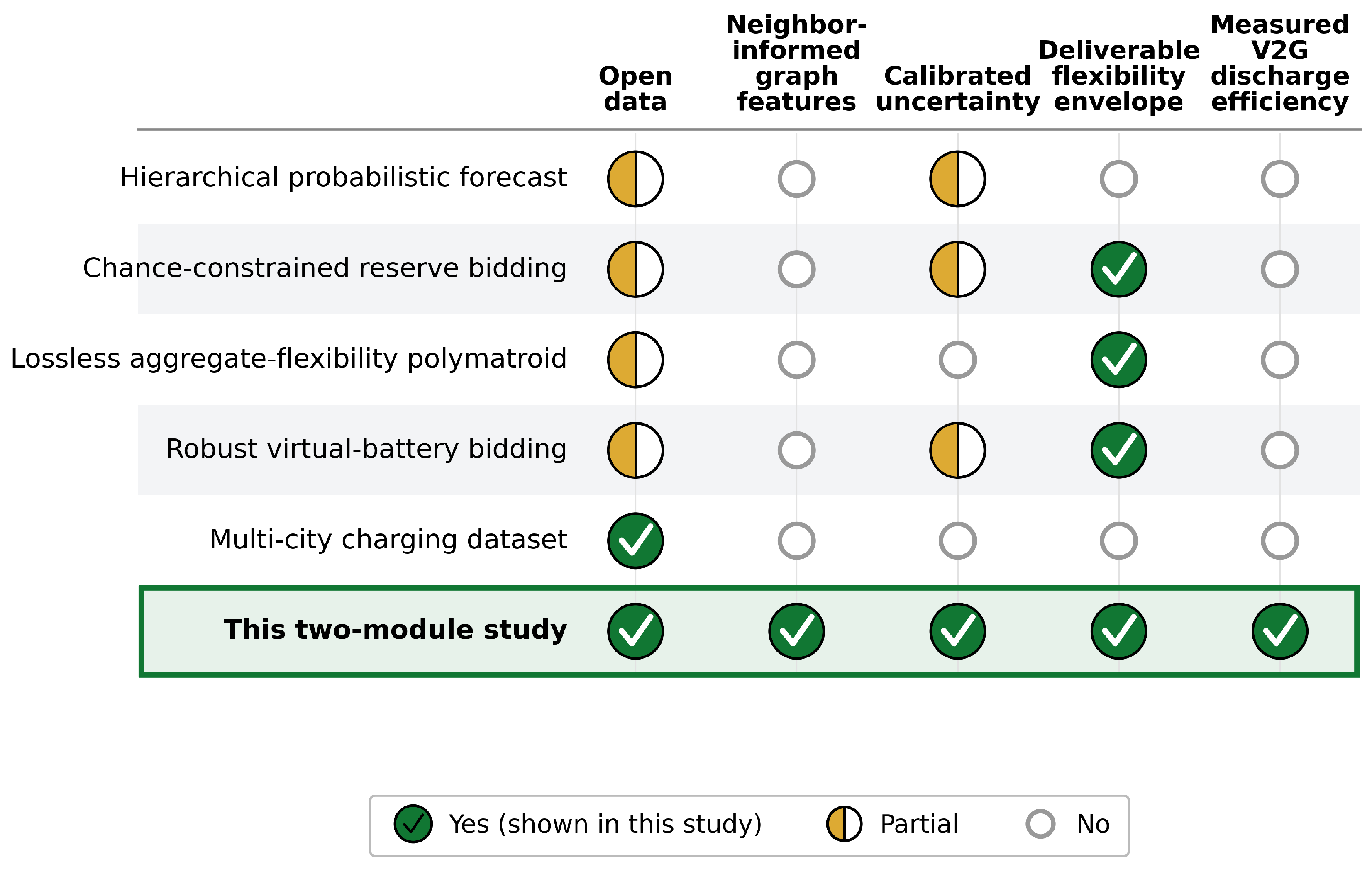
The second gap, more consequential, follows from the geometry line. The polymatroid and virtual-battery constructions that make the aggregate-feasible region convex rely on constant, state-independent loss assumptions. Where forecast uncertainty is propagated at all, it is routed into market and price variables. It is never routed into the device physics that determines how much energy a dispatch actually delivers. A feasible region drawn under a constant average efficiency therefore contains commitment points that cannot be honored. Because the error compounds with the depth and aggressiveness of the dispatch, the over-commitment is largest exactly when the flexibility is most valuable. A bidirectional-charging dataset with measured discharge traces suitable for closing this gap now exists in the open literature [27]. Operationalizing it inside a feasible-region model has not been done. The capability map in Figure 1 places this pair of gaps against the closest prior work. It shows that the pairing this study occupies, calibrated charging-demand uncertainty alongside a deliverable envelope built on measured efficiency, is unaddressed in the existing literature.

The objective of this study is to develop and validate, on public data, two complementary modules that address these gaps separately. The contribution is one of application rather than method invention. Split conformal calibration and inner-approximation geometry are established tools. What is new is where they are applied. The first application is a calibrated probabilistic charging forecaster that, to our knowledge, is the first to report interval coverage on a multi-zone EV benchmark. The second is a deliverable-envelope mechanism study, the first to place a measured, state- and rate-dependent V2G discharge efficiency inside a feasibility envelope. The forecasting module emits per-zone predictive distributions for the observable charging-demand target and calibrates them by conformalized quantile regression. The physics module fits V2G discharge efficiency as a function of state of charge and power from measured discharge traces. It builds a single convex polytope bounded on the discharge side by a decision-independent measured efficiency extremum. The charge side is held at a single conservative constant, so the two-sided measured band is exercised only where the V2G evidence lies. The polytope is a conservative inner approximation whose feasibility holds under the true efficiency provided that efficiency lies within the fitted admissible bounds. Deliverability is scored by an independent leave-one-vehicle oracle that replays commitments against a held-out vehicle’s raw measured trace. The conventional constant-average-efficiency aggregator is scored on the same oracle as the comparator the efficiency-aware envelope is meant to improve on. Each module is validated on its own data, on held-out records it never saw. The calibration claim and the deliverability claim can therefore each be falsified before they are combined. A co-located dataset that measures charging demand and V2G discharge on the same fleet is the named next validation. Closing the forecast-to-commitment loop into a single evaluated pipeline is left to future work.

The scope of this work is bounded to a two-module study on public data, a calibrated forecaster and a deliverable-envelope mechanism analysis, not a deployed aggregator. It does not price battery cycle-life degradation, model telemetry latency or automatic-generation-control signalling, resource-qualification scoring, settlement-baseline construction, or alternating-current network and AC/DC inversion effects. It also does not claim that laboratory efficiency curves are population-representative. The uncertainty quantified here is on the observable charging-demand target. Conformal coverage is claimed only for that metered quantity, while delivery compliance is reported as an empirical frequency rather than a distribution-free guarantee on a non-observable delivered-energy quantity. Efficiency uncertainty is carried separately, on the delivery side, by the measured admissible-efficiency band, and price and behavioral uncertainty is deferred to a downstream commitment-sizing layer.

Within these bounds the study makes two contributions, each carried by a principal finding. As a calibrated lightweight probabilistic baseline, the forecaster brings the prediction intervals inside the five-percentage-point coverage tolerance at both nominal levels. It also keeps the continuous ranked probability score below its conformalized-point counterpart at matched point accuracy. It is the first forecaster to report calibrated interval coverage on the multi-zone UrbanEV benchmark, where the published leading models report point error only. On the deliverability side, the contribution is that the efficiency-aware envelope’s residual delivery shortfall on held-out vehicles is smaller than the constant-average aggregator’s. The principal deliverability result is the full-state separation. The efficiency-aware envelope short-delivers less than the constant-average aggregator in every leave-one-vehicle fold from a commitment fraction of 0.95 onward. The mean gap is non-decreasing up to its peak and then declines as both plans saturate toward total shortfall. A separation of ten percentage points emerges only in an extreme corner combining over-commitment beyond measured capacity with the deepest depth of discharge, on three lab vehicles.

Section 2 describes the method. It covers the overall research strategy and the variables and data structures each module collects. It also covers the construction, calibration, and validation of the probabilistic forecaster and the efficiency-aware inner envelope. The data sources, collection windows, descriptive statistics, and preliminary processing are documented in Section 3. Section 4 presents and discusses the results, comparing the calibrated forecaster against its point baseline and the efficiency-aware envelope against the constant-efficiency aggregator across the commitment-stress sweep. It also analyzes the regime in which the over-commitment becomes operationally significant. Section 5 concludes with the study’s contributions, implications, limitations, and directions for future work.

2. Method

2.1. Methodological Framework

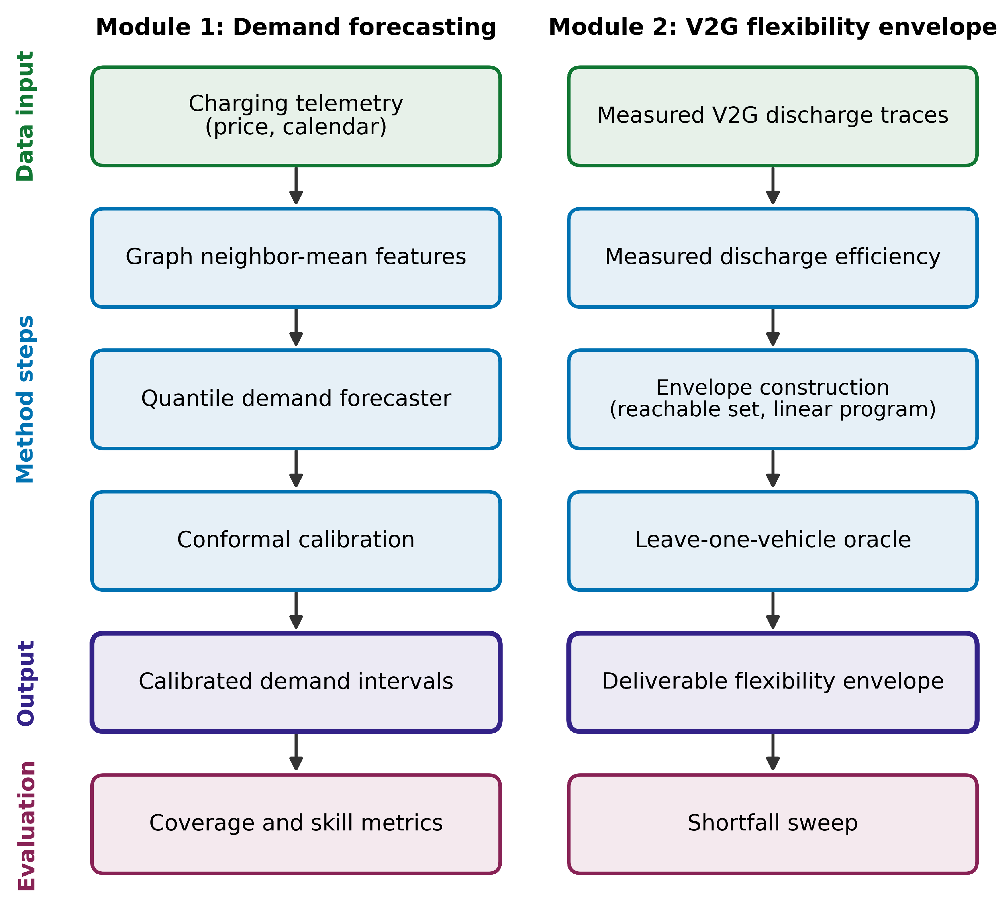
This study is executed as two methodological modules that draw on two public datasets and are evaluated on their own terms. The forecasting module consumes the UrbanEV zone charging telemetry together with its price and calendar context. Graph-informed neighbor-mean features summarize the surrounding zones. A gradient-boosted quantile-regression model turns those features into per-zone predictive distributions. A conformalized-quantile-regression step then calibrates those distributions into coverage-controlled demand intervals. The delivery module consumes the measured V2G discharge traces. The state- and rate-dependent discharge efficiency estimated from those traces parameterizes a deliverable V2G flexibility envelope, built as a decision-independent reachable-energy set and then a convex linear program. The envelope’s output is an inner V2G commitment band. The two modules share no input and are not chained into one forecast-to-delivery pipeline. Each produces its own module output from its own data. Figure 2 presents this framework as the data-to-method-to-output flow.

Two evaluation arms assess the two modules. The forecasting module is scored on the held-out UrbanEV test block for prediction-interval coverage and probabilistic skill against a conformalized point baseline at matched point accuracy. The delivery module is scored by a leave-one-vehicle deliverability oracle. The oracle replays the committed trajectories against the raw measured discharge of a held-out vehicle and reports the shortfall across a commitment-aggressiveness sweep. For comparison, a constant-average-efficiency aggregator undergoes the same procedure. Both arms read their result on data the corresponding module never saw, so coverage and shortfall are measured rather than assumed. The design choice that governs the study is the separation between what is claimed with a distribution-free guarantee and what is claimed empirically. Conformal coverage is asserted only for the observable forecast target, while delivery compliance is reported as a measured frequency against held-out hardware.

2.2. Data-Collection Method: Variables and Structure

The forecasting stage operates on the UrbanEV aggregate target. The structure is a matrix of hourly charging volume indexed by zone and time, restricted to the highest-volume zones over a recent window of the record. Each zone carries lagged values of its own history over a fixed look-back window. It also carries adjacency-weighted neighbor-mean features, formed by averaging neighboring zones’ lagged histories over the row-normalized zone adjacency. It also carries lagged occupancy and exogenous calendar and price signals at the target time. These are the engineered inputs from which the forecaster predicts the next-hour and day-ahead distribution. The data are partitioned strictly in time into training, calibration, and test blocks. The conformal calibration block and the test block are therefore out of sample relative to training. The zone count, window length, look-back length, partition fractions, and resulting instance counts are recorded with the data description.

The physics stage draws on a distinct measured quantity, the Esser bidirectional-charging dataset [27]. It records sub-second grid-side and vehicle-side voltage, current, power and state of charge for real electric vehicles. The bidirectional-capable vehicles supply the discharge traces that define the V2G efficiency model. The relevant variable is V2G discharge efficiency as a function of state of charge and power. It is estimated as the ratio of grid-side to battery-side energy within each state-of-charge decile rather than assumed. Each vehicle’s runs are further split by C-rate into a high-power and a low-power subset, selected by the power level recorded with each run file. Efficiency can then be stratified by discharge intensity. The vehicles, run counts, and power levels are recorded with the data description. This dataset is lab-scale by nature, so the measured efficiency curves are treated as device archetypes. The forecasting and physics datasets do not share a calendar window or a region. The two stages are therefore only conceptually aligned by time-of-day and seasonal structure rather than through a co-located demand-and-market record, and no absolute revenue is claimed.

2.3. Data-Analysis Method

The forecaster is a gradient-boosted regression model trained one quantile at a time. For each nominal quantile level a separate gradient-boosted tree ensemble minimizes the pinball loss for that level on the training block. The per-level predictions are sorted across levels so the emitted quantiles are monotone and do not cross. The model is fed engineered features rather than a learned graph. The features are each zone’s own-history lags and adjacency-weighted neighbor-mean lags that summarize the surrounding zones through the fixed row-normalized adjacency. They also include lagged occupancy, the forecast horizon, and the calendar and price signals at the target time. The spatial coupling between zones therefore enters the model as a neighbor-mean feature derived from the adjacency, not as a graph-convolution layer or a learned time-conditioned adjacency. The gain over a purely zone-by-zone model comes from this graph-informed feature together with the exogenous conditioning. The trees can exploit both without the cost or the calibration difficulty of a deep network. Point predictions are read from the median ensemble and are the quantity against which point accuracy is compared. A gradient-boosted point regressor trained on the identical feature table with a squared-error objective supplies the basis for the conformalized point baseline. The two models therefore differ only in their training objective.

The raw quantile ensemble is sharp but under-covers, so coverage is restored by CQR on the calibration block. For each nominal level the conformity score of a calibration instance is the signed amount by which the truth falls outside the predicted band. This score is the larger of the lower-quantile undershoot and the upper-quantile overshoot. The band is then widened by the empirical quantile of these scores at rank corresponding to the nominal level. The correction is applied to the observable charging target only. No coverage is claimed for any downstream non-observable quantity. A group-conditional variant calibrated separately by forecast horizon is computed alongside the pooled correction as a by-horizon check on whether a single pooled shift hides horizon-dependent miscalibration. The conformalized point baseline used for comparison is subjected to the identical split-conformal machinery. Any difference between the two therefore reflects the forecaster rather than the calibration step. Calibration is only useful if it neither degrades the underlying forecast nor restores coverage by inflating intervals. The calibrated forecaster and the conformalized point baseline are therefore scored on a fixed protocol that separates these effects. Probabilistic skill is read from the continuous ranked probability score and the mean pinball loss. Both reward a predictive distribution that is well-located and well-resolved, and both are reported in the same charging-volume units as the target. Sharpness is read from the normalized average interval width at each nominal level, so that a coverage gain cannot be bought by widening the band. Point accuracy is read from the mean absolute error of each model’s point prediction. The two forecasters are admitted to the skill comparison only when their relative point-accuracy gap stays within an iso-accuracy tolerance. This holds the center of the forecast fixed and attributes any probabilistic difference to the distribution rather than to a sharper median. The achieved coverage, skill, width, and point accuracy of these constructions are read on the held-out test block under this protocol.

The flexibility envelope is built from measured efficiency rather than a constant. It is constructed as a conservative inner approximation of the true feasible region, with a precise statement of what “inner” means. For each interval t and site, the decision variables are a non-negative charge power $p_t^c\ge 0$, a non-negative discharge power $p_t^d\ge 0$, and a stored-energy state $e_t$. Under the true but unknown charge and discharge efficiencies ${\eta }_c(·)$ and ${\eta }_d(·)$ the energy dynamics over an interval of length $\Delta$ are

$$e_{t+1}=e_t+{\eta }_c{p}_t^c\Delta -p_t^d\Delta /{\eta }_d.$$

(1)

The construction first computes a decision-independent reachable-energy set $R_t$ with lower and upper endpoints ${\underline{r}}_t$ and ${\overline{r}}_t$ for every interval. The endpoints are obtained by interval-propagating the dynamics from the initial-state range under a coarse outer efficiency interval and the box power limits alone. The set $R_t$ thus over-approximates every energy state the trajectory could occupy under any admissible decision. The discharge efficiency bounds ${\underline{\eta }}_d,{\overline{\eta }}_d$ govern the returnable V2G energy. They are read as the extrema of the measured discharge curves over the decision-independent partition cell that contains $R_t$ and the admissible power range. That cell is recorded in the released configuration. The charge-side bounds are set to a single conservative constant ${\eta }_c^{\mathrm{const}}$, so the charge-side band collapses to a point. The two-sided measured band is exercised only on the discharge side. This choice reflects that the deliverability evidence in this study and the delivery-shortfall mechanism it isolates lie entirely on the discharge side. Because these coefficients are fixed a priori, every constraint is affine and the feasible set is a single convex polytope solvable as a linear program. The polytope carries a two-sided energy band whose pessimistic floor and optimistic ceiling are

$$\begin{array}{cc}\hfill {\underline{e}}_{t+1}& ={\underline{e}}_t+{\eta }_c^{\mathrm{const}}{p}_t^c\Delta -p_t^d\Delta /{\underline{\eta }}_d,\hfill \end{array}$$

(2)

$$\begin{array}{cc}\hfill {\overline{e}}_{t+1}& ={\overline{e}}_t+{\eta }_c^{\mathrm{const}}{p}_t^c\Delta -p_t^d\Delta /{\overline{\eta }}_d,\hfill \end{array}$$

(3)

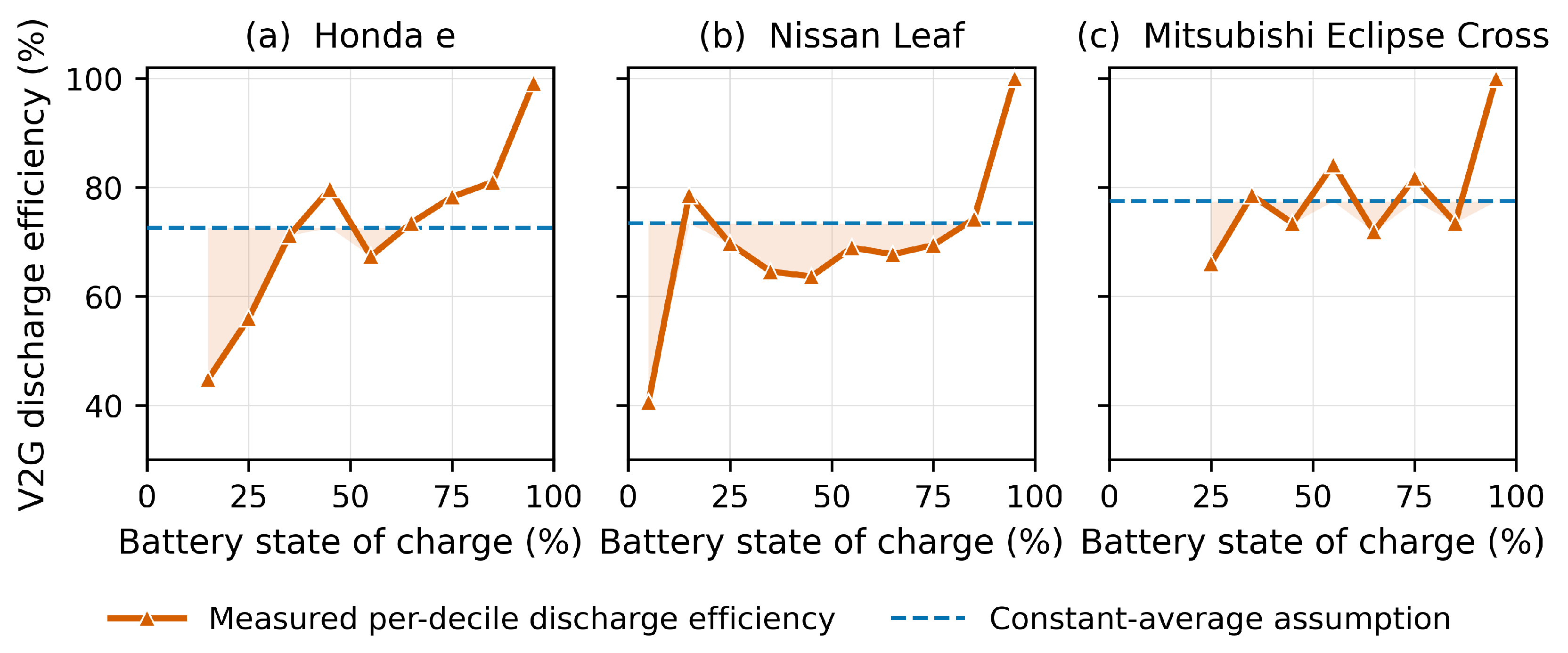
so the floor deposits at the single charge constant and discharges at the worst withdrawal efficiency, while the ceiling discharges at the best. The two-sided band is carried entirely by the measured discharge bounds. The construction is asymmetric. The discharge side carries the full measured band, while the charge side is held at the single conservative constant ${\eta }_c^{\mathrm{const}}$. A physical charging efficiency is itself state-of-charge dependent. Admitting its measured variation would replace the charge constant by a band lying at or below ${\eta }_c^{\mathrm{const}}$, tightening the envelope further. Fixing the charge side at one conservative constant therefore only removes deliverable energy from the plan. It cannot inflate the over-commitment gap the evaluation attributes to the discharge physics. Both edges are required to stay within the minimum and maximum state-of-charge operating limits, ${\mathrm{SoC}}_{min}\le {\underline{e}}_t$ and ${\overline{e}}_t\le {\mathrm{SoC}}_{max}$, at every interval. The inner-approximation statement follows from monotonicity. The charge side is fixed at the single conservative constant, and ${\underline{\eta }}_d\le {\eta }_d\le {\overline{\eta }}_d$ holds on each cell. The true energy state therefore obeys ${\underline{e}}_t\le e_t\le {\overline{e}}_t$ for every t under any feasible plan. A plan that keeps the band inside the operating limits therefore also keeps the true trajectory inside them. Any $(p^c,p^d)$ feasible in the polytope is therefore feasible under the true efficiency whenever that efficiency lies within the fitted bounds. Each constraint is bounded by its own correct extremum, the charge side by the conservative constant and the discharge lower limit by $1/{\underline{\eta }}_d$. This feasibility property is conditional, holding only when the fitted admissible efficiency set actually contains the held-out vehicle’s physics. The bounds are inflated by fit-residual and measurement-noise margins recorded in the released configuration to make that condition more realistic. The extra conservativeness from using $R_t$ rather than the realized band is treated separately as a partition gap. The inner-approximation property is thus a property of the construction given an admissible efficiency set. Whether that set contains held-out device physics, and therefore whether the inner envelope itself retains a residual shortfall, is the separate empirical question the leave-one-vehicle oracle answers. The measured V2G discharge efficiency curves against state of charge for the V2G-capable vehicles are shown in Figure 3. They exhibit the strong state and rate dependence the constant-efficiency assumption ignores.

The shaded regions indicate state-of-charge deciles in which the measured discharge efficiency falls below the constant-average assumption shown by the blue dashed line.

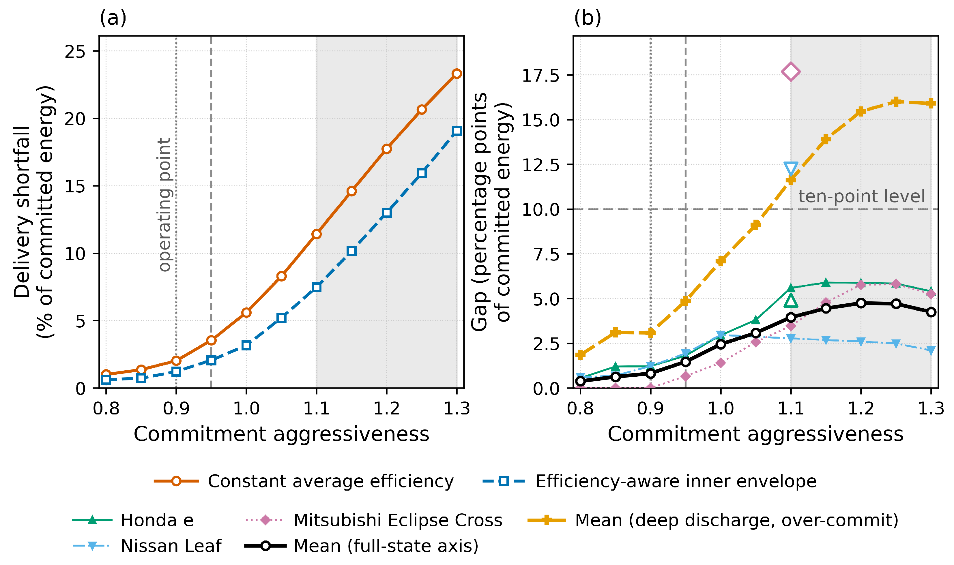
Deliverability is scored by a leave-one-vehicle oracle. The efficiency bounds are fit on all but one of the bidirectional vehicles. The resulting commitment is replayed against the raw measured discharge of the held-out vehicle, cycling through each in turn. The oracle ground truth is therefore always real hardware the envelope never saw. The evaluation isolates the deliverability mechanism fold by fold rather than estimating a fleet population, and every quantity below is read per held-out vehicle. The same procedure scores a constant-average-efficiency aggregator, the practitioner default. Its scalar efficiency is learned from the identical training information as the strongest state-independent constant the same data support. Both plans are compared at the same commitment input, and the delivery shortfall of each is the fraction of committed energy not returned. The comparison is reported as a curve over a grid of commitment aggressiveness relative to measured availability. Two further slices accompany it, a measured C-rate stratification into the high- and low-power subsets and a deep depth-of-discharge slice restricted to the lowest state-of-charge deciles. The grid range is anchored to the external one-way charge-discharge efficiency band reported by Bobanac, Bašić and Pandžić [28]. That band sets the plot range, while the per-decile efficiencies remain the measured Esser curves. The grid limits are recorded in the released configuration. The mechanism the evaluation is designed to expose is that a plan built on a single average efficiency over-promises grid energy and under-delivers. The efficiency-aware inner envelope commits less and short-delivers less than the constant-average plan. The constant-average plan’s shortfall should therefore exceed the inner envelope’s by a margin that grows as commitments become aggressive. The evaluation reports the direction of this margin fold by fold. It also reports the aggressiveness from which the direction holds in every fold and whether the mean gap is monotone in aggressiveness. The direction and its growth are treated as the robust finding and the magnitude as regime-dependent. The deep depth-of-discharge slice is reported as a separate overlay rather than as an operating-point result. It combines over-commitment beyond measured capacity with a dispatch restricted to the lowest state-of-charge deciles, and so carries a wide per-fold spread. The achieved direction, monotonicity, operating-point gap, and the magnitudes on the full-state, C-rate, and deep-discharge axes are read fold by fold. The full gap-versus-stress curve, with the primary commitment-aggressiveness axis and the deep-discharge over-commit regime drawn as a separate overlay, is shown in Figure 4.

3. Data

3.1. Data Sources, Collection Windows, and Descriptive Statistics

The study draws on two public datasets. The UrbanEV charging benchmark supplies the forecasting target, and the Esser measured bidirectional-charging dataset supplies the efficiency physics. Both are openly licensed, and no proprietary input enters the study. The descriptive statistics below cover these two in-scope datasets only.

The forecasting stage operates on UrbanEV [11], the open benchmark that now anchors zone-level EV charging forecasting. The dataset provides time-by-zone matrices of hourly charging volume, occupancy, and energy price for 275 traffic-analysis zones, a zone adjacency graph, and joined weather and point-of-interest features. The forecasting target used here is the hourly charging volume. It is restricted to the thirty zones with the highest mean charging volume over the full record, over the most recent 120 days. That window runs from 1 November 2022 to 28 February 2023 at one-hour resolution and yields a target array of 2880 time steps across 30 zones. Charging volume over this window has a mean of 1647 and a median of 859 in charging-volume units. The standard deviation of 2007 exceeds the mean, the signature of a right-skewed load that spikes far above its typical level. The maximum hourly zone volume reaches 15,329 while the floor is zero, and only half a percent of all zone-hours are exactly zero. The skew is spatial as well as temporal, with per-zone mean volume ranging from 380 in the quietest retained zone to 6270 in the busiest. This sixteen-fold spread is what the spatial graph is meant to exploit. Concurrent occupancy averages 39 simultaneously connected vehicles per zone and reaches 354 at the busiest zone-hour. The time-of-use energy price ranges from 0.238 to 1.354 RMB per kilowatt-hour with a mean of 0.877, the exogenous price signal the forecaster conditions on. The heavy right tail and the wide cross-zone dispersion are what make a single point forecast an inadequate basis for a commitment. The quantity an operator must bid against is the upper tail of this distribution, not its mean, and that tail is precisely what a point model leaves unstated.

The physics stage draws on a different measured quantity entirely. The Esser bidirectional-charging dataset [27] records sub-second grid-side and vehicle-side voltage, current, power, and state of charge for real electric vehicles on laboratory hardware. Three of the dataset’s vehicles are V2G-capable and supply the discharge traces that define the efficiency model, a Honda e, a Nissan Leaf, and a Mitsubishi Eclipse Cross. These are the only bidirectional-capable vehicles in the dataset, and the remaining vehicles charge in one direction only. Each contributes three measured discharge runs sampled at roughly two hertz. Individual runs span state of charge from near eight percent up to one hundred percent and last from about thirty-five minutes to nearly nine hours. Every vehicle carries both a high-power 10 kW run and a low-power 5 kW run, identified by the power level recorded with each run file. This provides the C-rate stratification used later. The efficiency these traces reveal is the feature the physics stage depends on. The self-calibrated discharge efficiency is estimated as the ratio of grid-delivered to battery-removed energy within each state-of-charge decile. It averages 0.726 for the Honda e, 0.734 for the Nissan Leaf, and 0.774 for the Mitsubishi Eclipse Cross. The per-decile values within a single vehicle range from below 0.45 at a low state of charge to near unity at a high state of charge. The spread is 34 to 59 percentage points across the state-of-charge axis. This is the state- and rate-dependent discharge loss that a single round-trip number cannot represent and that the envelope is built to respect. The dataset is laboratory-scale by nature. With three bidirectional vehicles, its efficiency curves are treated as device archetypes.

3.2. Preliminary Data Processing

The UrbanEV matrices are aligned and subset before any model sees them. The volume, occupancy, and price matrices are checked to share an identical time index and zone-column order. Subsetting keeps the thirty zones with the highest mean charging volume over the full record and the most recent 120 days. The source matrices are verified free of missing values, with a forward-fill-then-zero guard applied as a safeguard so that no spurious volume is introduced. Each zone’s representation then combines lagged values of its own history over a 24 h window with neighbor-mean features derived from the adjacency graph and the calendar exogenous signals. The series is partitioned strictly in time into 60 percent for training, 20 percent for conformal calibration, and 20 percent for testing. These are contiguous calendar spans. Training runs from 2 November 2022 to 12 January 2023 at 09:00. Calibration runs from 12 January 2023 at 10:00 to 5 February 2023 at 04:00. Testing runs from 5 February 2023 at 05:00 to 28 February 2023 at 23:00. The calibration and test blocks are adjacent with no gap between them, which supports the exchangeability assumption underlying the conformal step. This temporal split keeps the calibration and test blocks out of sample relative to training and is what makes the conformal coverage claim a genuine held-out result. Across zones and forecast horizons, the partition yields 34,260 calibration instances and 33,570 test instances. The horizons evaluated are the next hour and the day-ahead step, and the quantile grid spans the central levels needed to construct the 80 and 90 percent intervals.

The Esser traces require more careful preparation because the raw meters are not directly comparable. The merged run files are semicolon-delimited with a units row that is dropped on read. The live state-of-charge channel is selected as the connector channel with the largest observed range, and the sample period is recovered from the millisecond epoch column. For each discharging sample, the grid-delivered energy is computed from the signed grid power over the sample interval and the battery-removed energy from the paired battery-capacity channel. Both are accumulated into the state-of-charge decile of the sample. A per-vehicle self-calibration is then applied. For some vehicles, the raw grid-to-battery ratio exceeds the physical unit-efficiency ceiling, an impossibility for a one-way discharge that signals a constant scale error in the battery-side meter. Each vehicle’s battery-removed energy is therefore rescaled by its own maximum raw per-decile ratio so that its best decile sits at or just below the unit-efficiency ceiling. The rescaled best decile is 1.00 for two of the three vehicles and 0.99 for the Honda e. This correction uses no external or assumed number, only the vehicle’s own measured grid power and reported capacity. It preserves the measured shape of efficiency across state of charge while removing the meter offset. The C-rate stratification is performed by selecting the matching run files by their recorded power level. The high- and low-rate subsets are therefore real measured files, and the stratification overrides no efficiency value. Throughout, the oracle ground truth is always the raw measured discharge trace of a held-out vehicle, never a fitted curve.

Every quantity reported in this study is reproducible from a single configuration recorded with the published results, under the seed value 20,240,601. The pipeline involves no stochastic sampling. The temporal split is deterministic, the gradient-boosted ensembles use neither row nor feature subsampling, and the leave-one-vehicle folds enumerate all three vehicles. The reported numbers therefore come from this single seeded run rather than from an average over repeated runs. The configuration includes the random seed, the temporal train/calibration/test fractions, and the quantile and nominal-coverage grids. It also records the per-quantile gradient-boosted forecaster’s 300 trees, 31 leaves per tree, and 0.05 learning rate. These are the standard LightGBM defaults, adopted to keep the probabilistic baseline lightweight and reproducible rather than tuned to this dataset. A sensitivity analysis confirms that interval coverage and forecast skill stay robust across the surrounding hyperparameter neighborhood. It also records the commitment-aggressiveness grid spanning 0.80 to 1.30 of measured availability and the depth-of-discharge windows.

4. Results and Discussion

The results reported here are bounded by the analysis framework of the two-module study. The forecasting results are the coverage and skill of the calibrated quantile model against its conformalized point baseline on the held-out UrbanEV test block. That block is the final 20 percent of the thirty-zone, 120-day hourly window under the strict temporal split, 33,570 instances pooled over the next-hour and day-ahead horizons. The deliverability results are the shortfall of the efficiency-aware inner envelope against a constant-average-efficiency aggregator on the leave-one-vehicle raw-Esser oracle over the three V2G-capable vehicles. They are read across the commitment-stress sweep recorded in the released configuration, with the measured high- and low-C-rate subsets and the deep depth-of-discharge windows as separate slices. Each subsection reports the construction, the validation against held-out data, and the comparison that gives the number its meaning. The commitment-value layer that would consume these distributions and the out-of-region market stress are out of the present scope, so no realized-revenue figure is reported.

4.1. Calibrated Coverage on the Open Benchmark

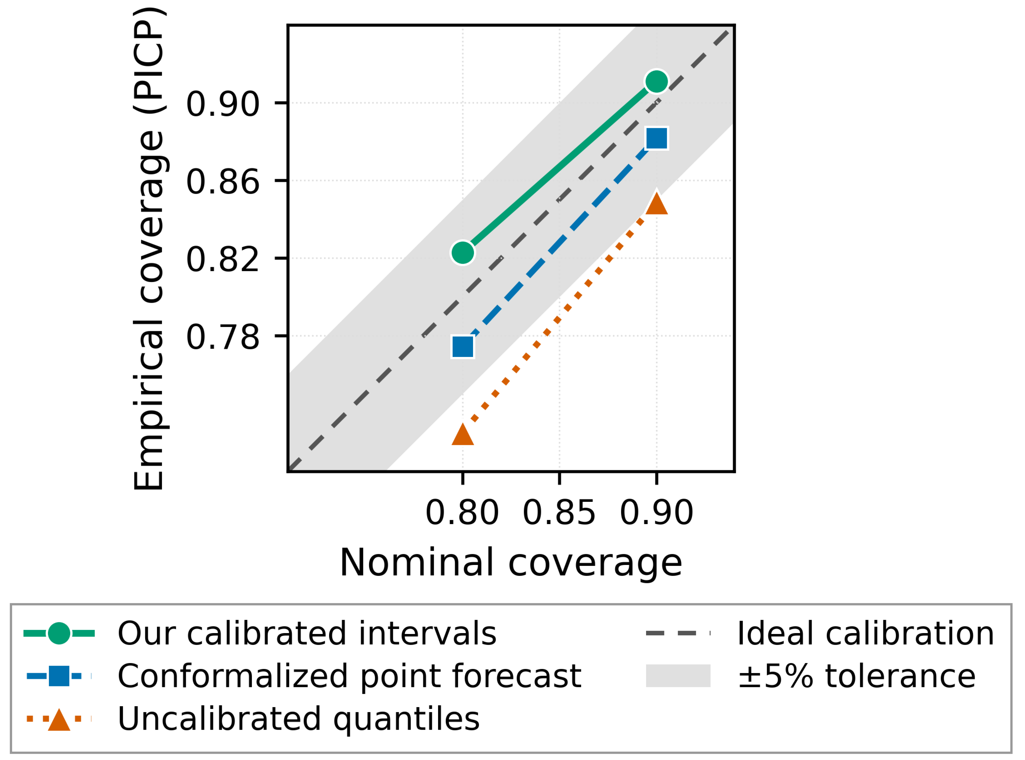
The first result is that conformalized quantile regression brings the prediction intervals inside the recorded coverage tolerance at both nominal levels. It supplies a calibrated probabilistic baseline on a benchmark whose published leading models report only point error and no calibration metrics. The strongest UrbanEV forecasters are point-only or coverage-silent. Graph WaveNet [4] and AGCRN [5] emit a point prediction. Although DeepAR [14] produces a parametric distribution, neither it nor the point-accuracy leader TimeXer [10] reports interval coverage on this benchmark. Re-running them would therefore not yield a calibrated comparator. The internal contrast is instead drawn against a conformalized-point forecaster at matched point accuracy. A matched-coverage head-to-head against these spatiotemporal and probabilistic models is set out as future work. The raw quantile ensemble is sharp but under-covers the expected behavior of a model trained on pinball loss without a calibration step. Before the conformal step, its measured coverage is 0.730 at the 80 percent level and 0.849 at the 90 percent level. These deviations of 0.070 and 0.051 both fall outside the five-percentage-point tolerance. Applying the conformal correction on the held-out calibration block and measuring on the test block, the 80 percent interval reaches a prediction-interval coverage probability of 0.823. The deviation from nominal is 0.023, which sits inside the five-percentage-point tolerance. The 90 percent interval reaches 0.911, a deviation of 0.011 that sits inside it. The pooled correction already meets the coverage tolerance at both levels, and the group-conditional variant calibrated separately by forecast horizon gives near-identical coverage, 0.822 and 0.911. Calibrating by horizon therefore confers no additional benefit here and confirms the pooled correction is not masking a horizon-dependent miscalibration. Figure 5 carries the coverage evidence for this calibrated-baseline claim, plotting the reliability of the three interval constructions against the ideal coverage line and the tolerance band.

The comparison that gives this number its weight is against the conformalized point baseline. That baseline is subjected to the identical split-conformal machinery, so the contrast isolates the forecaster rather than the calibration procedure. That baseline covers 0.774 and 0.882 at the two levels. Its deviations from nominal of 0.026 and 0.018 stay inside the five-percentage-point tolerance but are larger than the calibrated model’s. The calibrated model is the closer of the two to nominal at both levels. The difference in behavior traces to where the two constructions place interval width. The calibrated quantile model inherits a heteroscedastic band from its quantile ensemble, widening where the conditional distribution is wide and tightening where it is narrow. A single conformal shift therefore suffices to align coverage. The point baseline carries a band of nearly constant width that a conformal shift can only translate, not reshape. The band therefore cannot simultaneously cover the heavy-tailed high-demand hours and avoid over-covering the quiet ones. It under-covers because the residual distribution it is calibrated against is dominated by the right tail of the demand. This is the practical content of calibrating on the observable target. Coverage is controlled on the quantity actually predicted. It is controlled because the quantile ensemble already encodes the demand-dependent spread that a constant-width interval cannot.

The correction is also insensitive to how much held-out data calibrates it. With the training block fixed and the calibration fraction swept from 0.15 to 0.30, coverage stays inside the tolerance at both levels. Coverage is 0.825 and 0.911 at 0.15, 0.823 and 0.911 at 0.20, 0.817 and 0.906 at 0.25, and 0.802 and 0.897 at 0.30. The continuous ranked probability score is lower than the point baseline at every fraction. The choice of correction matters more than its size. The raw ensemble at 0.730 and 0.849 is the only construction outside tolerance, while the conformal correction and the horizon-conditional Mondrian variant both pass.

4.2. Probabilistic Skill at Matched Point Accuracy

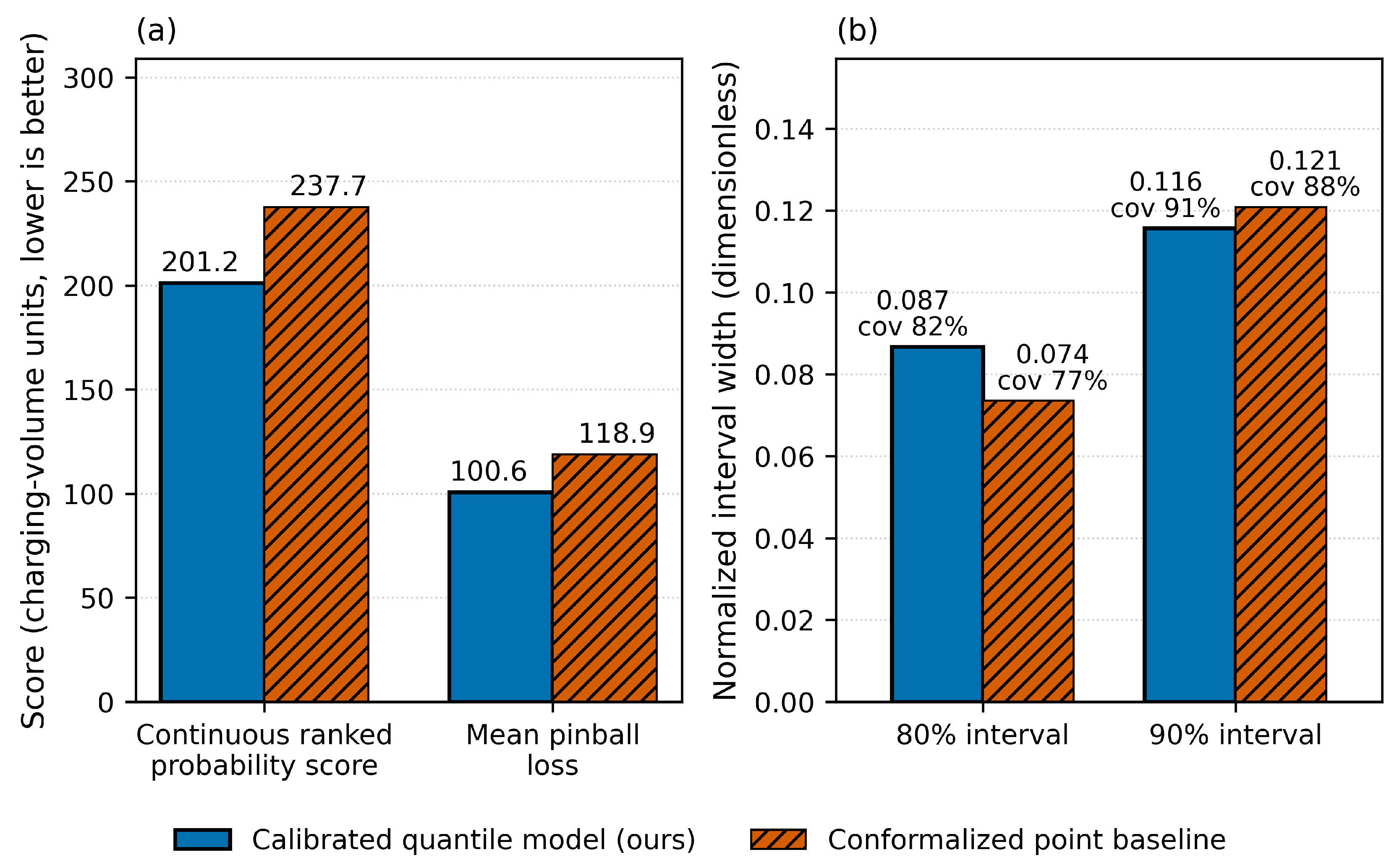
Calibration is only valuable if it neither inflates intervals nor degrades the underlying forecast. The second result is that the calibrated forecaster improves on probabilistic skill over its conformalized-point counterpart while matching point accuracy. The continuous ranked probability score rewards a predictive distribution that is both well-located and well-resolved. It falls from 237.7 for the conformalized point baseline to 201.2 for the calibrated quantile forecaster, a reduction of roughly fifteen percent. The raw quantile model before calibration scores 201.7, so the conformal correction preserves the skill advantage intact while fixing coverage. The mean pinball loss tells the same story, dropping from 118.9 to 100.6. Both scores are in the same charging-volume units as the forecast target, whose mean over the window is 1647, so the magnitudes are interpretable on the load scale. Normalized by that mean, the continuous ranked probability score is 0.122 for the calibrated forecaster against 0.144 for the baseline. Figure 6 carries the skill and width evidence for the calibrated-baseline claim.

The skill gain is not bought with point error, and it is not bought with width. Mean absolute error is 338.35 for the calibrated forecaster against 346.61 for the baseline. The relative gap of 2.38 percent stays within the five percent iso-accuracy threshold used to declare matched point accuracy. The two models are therefore compared at genuinely matched point performance, and the probabilistic advantage is attributable to the distribution, not to a sharper center. Nor does the calibrated model achieve coverage by the trivial route of widening intervals. At the 90 percent level its normalized average interval width is 0.116 against the baseline’s 0.121. It is therefore the narrower of the two while also being the better-covered. At the 80 percent level, its width of 0.087 is the modest price of moving coverage from 0.774 to 0.823. The calibrated model can be simultaneously sharper, better-covered, and equally accurate at the center. The reason is that the score it minimizes and the coverage it is calibrated for act on different aspects of the same heteroscedastic band. The quantile ensemble resolves where the uncertainty actually is, the conformal step certifies the resulting coverage, and the median is left untouched. A constant-width interval has to trade these objectives against one another, which is why the baseline pays in coverage what it saves in modelling effort.

These properties hold across the forecaster’s configuration and under moderate data loss.

Table 1. Forecaster diagnostics across configuration and data-deficiency conditions on UrbanEV.

Configuration	PICP@80%	PICP@90%	CRPSours	CRPSbase	MAEours
Default (300 trees, 31 leaves, learning rate 0.05)	0.823	0.911	201.19	237.70	338.35
150 trees	0.820	0.912	208.36	240.75	348.42
600 trees	0.822	0.912	197.99	237.53	333.18
15 leaves	0.823	0.913	208.42	243.22	349.59
63 leaves	0.818	0.911	197.86	235.63	332.74
learning rate 0.03	0.820	0.911	205.48	238.99	344.68
learning rate 0.10	0.822	0.912	198.85	237.85	334.45
5% missing (MCAR)	0.817	0.908	209.50	249.20	350.99
10% missing (MCAR)	0.826	0.909	216.16	260.04	365.32

PICP is the prediction-interval coverage probability. CRPS is the continuous ranked probability score, in charging-volume units. Subscript ’ours’ marks the calibrated forecaster and ’base’ the conformalized point baseline.

sweeps the gradient-boosted model over a neighborhood of its tree count, leaf count, and learning rate. Every cell keeps coverage inside the five-percentage-point tolerance at both nominal levels and improves on the point baseline on the continuous ranked probability score. The lightweight default lands within about 1.6 percent of the best-scoring cell. The calibrated-coverage result is therefore a property of the construction rather than of a tuned setting. Robustness to data deficiency follows the same pattern. Under seeded missing-completely-at-random loss repaired by the forward-fill-then-zero guard, coverage stays inside the tolerance at both five and ten percent missing. The continuous ranked probability score still improves on the point baseline (Table 1).

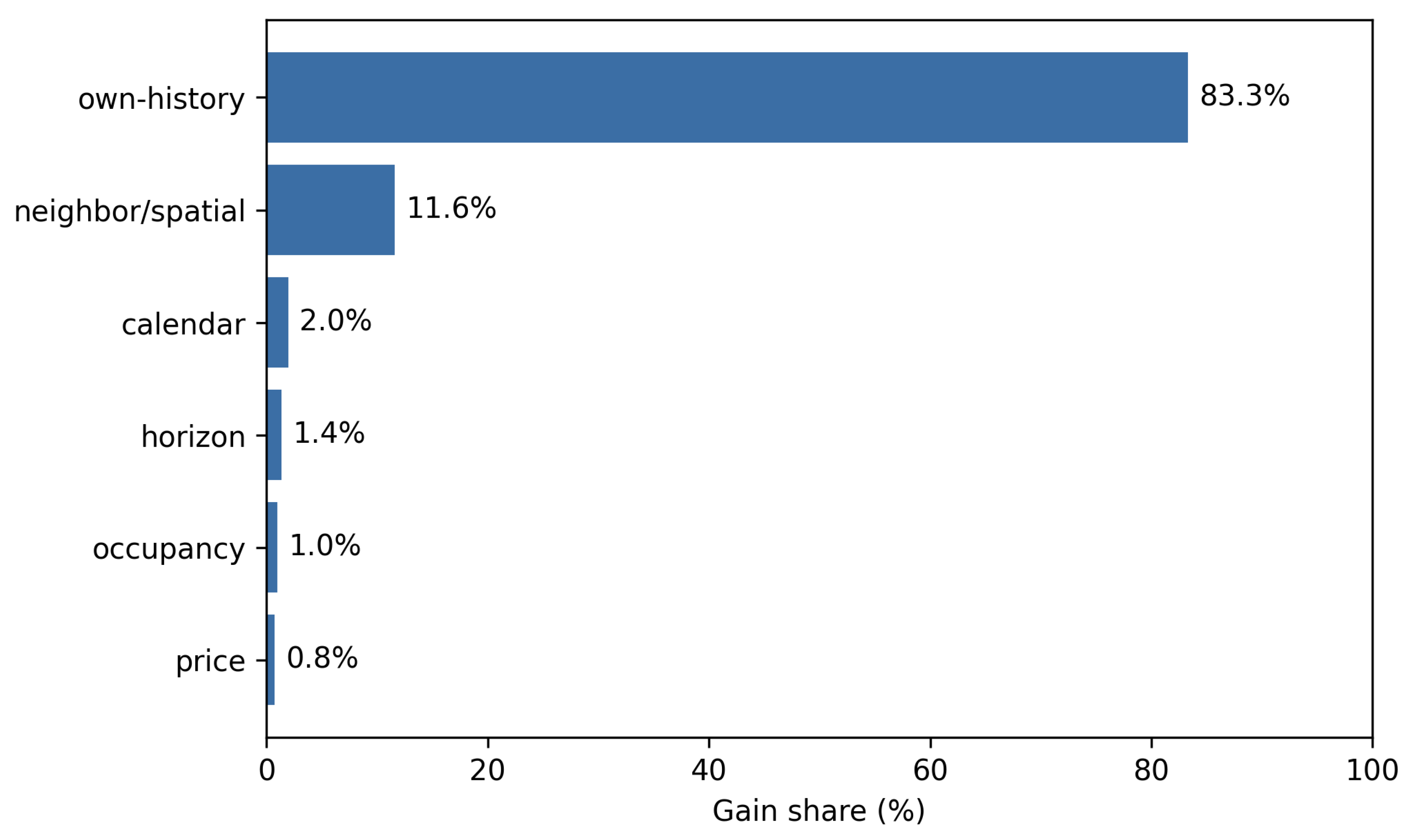
Recent own-history dominates the gradient-boosted quantile forecaster, contributing 83.3 percent of the model gain in the feature-importance decomposition of Figure 7. The graph-informed neighbor-mean and spatial family ranks second at 11.6 percent, corroborating the adjacency features that stand in for a learned graph. This concentration of gain in own-history together with a static neighbor-mean is why the engineered features suffice in place of a learned time-conditioned adjacency.

4.3. The Measured-Physics Deliverability Mechanism on Three Bidirectional Vehicles

Across the three V2G-capable vehicles in the Esser dataset, a constant-average-efficiency aggregator over-promises grid energy and under-delivers. It under-delivers more than the efficiency-aware inner envelope does. The inner envelope’s residual shortfall is therefore the smaller of the two. The direction and growth of this margin, rather than any single magnitude, are the robust finding. The comparator is the practitioner default, a scalar-efficiency plan whose round-trip number is learned from the same training information as the strongest state-independent discharge scalar. It is thus the strongest version of the conventional shortcut the same training information supports. Both plans are scored on the leave-one-vehicle oracle, with efficiency bounds fit on two vehicles and the commitment replayed against the raw measured discharge of the held-out third. Both are read at the same commitment input across the aggressiveness grid. The cause of the gap is the state-of-charge dependence of discharge efficiency drawn in Figure 3. Discharge efficiency collapses toward the lowest states of charge because a cell’s open-circuit voltage falls as it empties. Returning a fixed grid power then demands a higher current, and ohmic and polarization losses claim a growing share of the energy withdrawn. This is exactly the state and rate dependence the independent cell-level studies report [20,21]. Because the measured curves fall this way, a plan that assumes the fleet-average efficiency promises energy the battery cannot return once the dispatch reaches those states. The inner envelope, by contrast, bounded by the conservative per-decile extremum, commits less into that loss and so short-delivers less.

The direction and monotonicity of the mechanism are confirmed on real held-out hardware. Once the commitment reaches measured availability, the constant-average shortfall exceeds the inner-envelope shortfall in each of the three leave-one-vehicle folds. This ordering holds fold by fold at every commitment fraction from 0.95 onward. Within each fold, the gap grows with aggressiveness up to its peak. With three vehicles, this is a mechanism demonstration, reported per fold, so no population or significance claim is attached to it. At the conservative operating point, a commitment fraction of 0.90 where the plan stays below measured availability, the mean shortfall gap is 0.81 percentage points. This decomposes into nearly coincident per-fold gaps of 1.215 points for the Honda e and 1.219 for the Nissan Leaf. The Mitsubishi Eclipse Cross shows a zero-versus-zero tie that resolves into a positive gap at 0.95. At this point, the constant-average plan already short-delivers 2.03 percent of committed energy against the inner envelope’s 1.21 percent. The gap is small here because at a conservative commitment, neither plan is pushed into the deep-discharge regime where the state-dependence of efficiency becomes pronounced. The two therefore behave similarly, and the shortfall is latent, not active, at this operating point. Figure 4 carries the deliverability evidence for the envelope claim.

The reported magnitude is the full-state separation, the shortfall gap between the constant-average plan and the inner envelope over the whole discharge range. Its mean gap on the full-state axis is non-decreasing up to a peak of 4.75 percentage points at a commitment fraction of 1.20. It then declines slightly as both plans saturate toward total shortfall. The C-rate slices behave the same way, with the high-power slice peaking at 4.33 points and the low-power slice at 4.83 points. This full-state margin, growing as the commitment is pushed beyond measured availability, is the principal deliverability finding. The ten-percentage-point figure illustrates how the bias compounds when two stresses act together on the three lab vehicles. One is over-commitment beyond measured capacity at a fraction of 1.10 or higher, and the other a dispatch restricted to the deepest state-of-charge deciles. In that corner at a commitment fraction of 1.10, the three leave-one-vehicle folds spread widely. The Mitsubishi fold reaches a gap of 17.7 points off an inner shortfall near zero. The Nissan fold reaches a gap of 12.2 points off an inner shortfall near 1.3 percent. The Honda e fold still retains a 4.9-point margin. Its held-out discharge is lossy enough to leave the inner envelope about 32 percent short in this deepest regime. The dispersion follows from where each held-out vehicle’s deep-decile efficiency sits relative to the bound fit on the other two. The Mitsubishi, the most efficient of the three, stays inside the conservative bound fit on its two less efficient companions. Its inner shortfall is therefore near zero, and the constant-average plan’s entire shortfall registers as a gap. The Honda e, the least efficient, falls below even that conservative bound in the deepest deciles, which compresses the margin between the two plans. Even there, the envelope still short-delivers less than the constant-average plan. Averaging this three-vehicle dispersion gives the derived deep-discharge mean gap of 11.6 points at that fraction, which rises to 16.0 points at 1.25. Widening the deep-discharge window from the lowest three deciles to the lowest four and five pushes the crossover later, to fractions of 1.15 and 1.20, respectively. The mechanism works as the physics predicts, with the inner envelope shortfalling less than the constant-average plan. The deepest states of charge and highest C-rates are where the constant-average plan over-commits most. These are also the operating regimes that cell-level studies identify as most damaging to battery life [20,21], and the efficiency-aware envelope commits least into them. The dispersion across three vehicles is large, however, so this corner is presented as an illustration rather than an operating-point result.

The shortfall gap might depend on defining the inner-envelope lower efficiency bound as the per-decile minimum. Re-fitting the bound at the 5th and 10th per-decile percentile settles the question. At the conservative operating point, the shortfall-gap direction is preserved under every variant and never reverses, each read against the same constant-average shortfall (

Table 2. Envelope lower-bound sensitivity at the conservative operating point (commitment fraction 0.90).

Inner-Envelope Lower Bound	Inner Shortfall (%)	Constant-Average Shortfall (%)	Gap (pp)
Per-decile minimum	1.21	2.03	0.81
5th percentile	1.28	2.03	0.75
10th percentile	1.36	2.03	0.66

Gap is the constant-average shortfall minus the inner-envelope shortfall in percentage points, computed at full precision, so it can differ from the rounded column difference by 0.01.

). The sensitivity is mild by construction. Each leave-one-vehicle fold trains on only two vehicles, so within a decile the 5th and 10th percentile nearly coincide with the minimum.

4.4. What Constrains Deliverable Flexibility

Read together, the three results locate the source of deliverable EV flexibility in the two places the conventional pipeline leaves unguarded. The forecasting result shows that calibrated uncertainty is attainable on the open benchmark at matched point accuracy. The calibration gain is not obtained by blanket interval inflation. The 90 percent interval is actually narrower than the under-covering point baseline, while the 80 percent interval widens only modestly to restore coverage. This removes the first obstacle to a commitment carrying a defensible probability. The comparison against the point baseline shows that the gain comes from resolving demand-dependent spread, not from a better-centered forecast. A point model, however accurate, therefore cannot supply it. The deliverability result identifies the constant-efficiency assumption as a directional over-commitment that grows with dispatch aggressiveness and depth of discharge. Fold by fold, this gap is largest exactly where the measured discharge efficiency falls furthest below its average. The two findings reinforce a single conclusion for an operator. Calibrated uncertainty on the observable load and measured V2G discharge physics on the delivery side each place a material constraint on deliverability that the separately evaluated modules expose. The forecasting model on its own, however it ranks on point error, addresses neither constraint. This is also why the shortfall matters most in the aggressive, deep-discharge dispatches. Those are the ones the constant-efficiency assumption mis-sizes the worst. That regime is the one the gap-versus-stress curve in Figure 4 isolates.

5. Conclusions

This study examined two defects that each limit deliverable EV flexibility. Charging-demand forecasts are reported without calibrated uncertainty, and the V2G dispatch that would consume them assumes a constant round-trip efficiency the underlying physics does not obey. Each is separately addressable, and each is established here as a distinct building block. Conformalized quantile regression runs on a gradient-boosted quantile forecaster with graph-informed neighbor features. It brings empirical coverage to within the five-percentage-point tolerance of its nominal target across the thirty-zone public benchmark. It improves the continuous ranked probability score over a conformalized point forecaster of comparable point accuracy. It also attains the smaller normalized interval width at the higher nominal level, so calibration is not bought through inflated bands. On the delivery side, the envelope is built from measured state- and rate-dependent V2G discharge efficiency. It short-delivers less than the constant-average-efficiency rule in every leave-one-vehicle fold from a commitment fraction of 0.95 onward. The full-state mean margin widens to a peak of 4.75 percentage points as commitments grow more aggressive. A small residual shortfall persists only where a held-out vehicle’s physics falls below the fitted bound.

The findings relocate the obstacle to a bankable EV commitment away from the accuracy frontier the forecasting literature competes on and into two properties that frontier leaves unaddressed. The first is calibrated coverage on the observable load, which a simple quantile model made conformal supplies. The second is a feasible region whose returnable energy follows measured rather than assumed discharge physics. For practice, this over-commitment is largest in the aggressive, deep-discharge dispatches. An aggregator pricing reserve on a single round-trip number is therefore most exposed in exactly those regimes. The indicated remedies are a measured efficiency band and an offer sized against a calibrated distribution.

The measured-physics result rests on three bidirectional vehicles, so the deliverability effect is a per-fold mechanism curve, not a population effect size. The per-fold spread in the deep-discharge over-commit regime is wide. Its mean is carried by folds whose inner-envelope shortfall is near zero, while the constant-average rule commits well beyond deliverable energy. The efficiency model is discharge-only, with the charge side held at a single conservative constant, and the lab-scale curves act as conservative device archetypes rather than fleet-representative distributions. The two modules are building blocks validated separately, with no closed-loop coupling evaluated. Conformal coverage is asserted only for the observable forecast target, and delivery compliance is an empirical frequency rather than a distribution-free guarantee. The market-value comparison, cross-city transfer, network-constrained dispatch, and degradation cost lie outside the present scope.

These limits set the follow-on work. The most decisive is a co-located dataset that measures charging demand and bidirectional discharge on the same fleet over the same window. Such synchronized traces let the forecast and the envelope be tested as one system rather than validated in isolation. Transfer learning and hierarchical-Bayesian partial pooling across chemistries would widen the measurement base beyond three vehicles. This would turn the per-fold over-commitment mechanism into a fleet-population estimate with stated uncertainty. A second forecasting direction is to conformalize TimeXer, Graph WaveNet, AGCRN, DeepAR, and DiffPLF on the same UrbanEV split. Testing the calibrated model against these spatiotemporal and probabilistic state-of-the-art forecasters under matched coverage would go beyond its point counterpart. Closing the forecast-to-commitment loop would feed the calibrated conformal quantiles into the specified but unevaluated commitment-sizing layer. That layer is a mean-minus-CVaR scenario program in the Rockafellar–Uryasev reformulation. This step would handle online exchangeability under decision-driven shift and scenario reduction. It would then score realized risk-adjusted value against deterministic, stochastic, robust, and learning-based baselines. Extending the envelope with cycle-life degradation cost, telemetry latency, and AC/DC inversion losses would sharpen it further. Each pushes delivered energy short in the same direction as the measured efficiency loss. The efficiency-aware envelope already commits least into the deep-discharge, high-rate regimes they penalize most. A fuller cost model therefore reinforces the reported gap rather than reversing it. Cross-city adaptive conformal correction, network constraints, and market-qualification rules would then carry the framework toward an operationally faithful aggregator that still reports a guarantee only where observable.

References

1. Li, Y.; Yu, R.; Shahabi, C.; Liu, Y. Diffusion convolutional recurrent neural network: Data-driven traffic forecasting. arXiv 2017, arXiv:1707.01926. [Google Scholar]
2. Yu, B.; Yin, H.; Zhu, Z. Spatio-temporal graph convolutional networks: A deep learning framework for traffic forecasting. arXiv 2017, arXiv:1709.04875. [Google Scholar]
3. Guo, S.; Lin, Y.; Feng, N.; Song, C.; Wan, H. Attention based spatial-temporal graph convolutional networks for traffic flow forecasting. In Proceedings of the AAAI Conference on Artificial Intelligence, Honolulu, HI, USA, 27 January–1 February 2019; Volume 33, pp. 922–929. [Google Scholar]
4. Wu, Z.; Pan, S.; Long, G.; Jiang, J.; Zhang, C. Graph WaveNet for deep spatial-temporal graph modeling. arXiv 2019, arXiv:1906.00121. [Google Scholar]
5. Bai, L.; Yao, L.; Li, C.; Wang, X.; Wang, C. Adaptive graph convolutional recurrent network for traffic forecasting. Adv. Neural Inf. Process. Syst. (NeurIPS) 2020, 33, 17804–17815. [Google Scholar]
6. Wu, Z.; Pan, S.; Long, G.; Jiang, J.; Chang, X.; Zhang, C. Connecting the dots: Multivariate time series forecasting with graph neural networks. In Proceedings of the 26th ACM SIGKDD International Conference on Knowledge Discovery & Data Mining, Virtual Event, San Diego, CA, USA, 23–27 August 2020; pp. 753–763. [Google Scholar]
7. Nie, Y.; Nguyen, N.H.; Sinthong, P.; Kalagnanam, J. A time series is worth 64 words: Long-term forecasting with transformers. arXiv 2022, arXiv:2211.14730. [Google Scholar]
8. Wu, H.; Hu, T.; Liu, Y.; Zhou, H.; Wang, J.; Long, M. TimesNet: Temporal 2D-variation modeling for general time series analysis. arXiv 2022, arXiv:2210.02186. [Google Scholar]
9. Liu, Y.; Hu, T.; Zhang, H.; Wu, H.; Wang, S.; Ma, L.; Long, M. iTransformer: Inverted transformers are effective for time series forecasting. In Proceedings of the International Conference on Learning Representations 2024 (ICLR 2024), Vienna, Austria, 7–11 May 2024. [Google Scholar]
10. Wang, Y.; Wu, H.; Dong, J.; Qin, G.; Zhang, H.; Liu, Y.; Qiu, Y.; Wang, J.; Long, M. TimeXer: Empowering transformers for time series forecasting with exogenous variables. Adv. Neural Inf. Process. Syst. (NeurIPS) 2024, 37, 469–498. [Google Scholar] [CrossRef]
11. Li, H.; Qu, H.; Tan, X.; You, L.; Zhu, R.; Fan, W. UrbanEV: An open benchmark dataset for urban electric vehicle charging demand prediction. Sci. Data 2025, 12, 523. [Google Scholar] [CrossRef] [PubMed]
12. Kuang, H.; Qu, H.; Deng, K.; Li, J. A physics-informed graph learning approach for citywide electric vehicle charging demand prediction and pricing. Appl. Energy 2024, 363, 123059. [Google Scholar] [CrossRef]
13. Wang, S.; Li, Y.; Shao, C.; Wang, P.; Wang, A.; Zhuge, C. An adaptive spatio-temporal graph recurrent network for short-term electric vehicle charging demand prediction. Appl. Energy 2025, 383, 125320. [Google Scholar] [CrossRef]
14. Salinas, D.; Flunkert, V.; Gasthaus, J.; Januschowski, T. DeepAR: Probabilistic forecasting with autoregressive recurrent networks. Int. J. Forecast. 2020, 36, 1181–1191. [Google Scholar] [CrossRef]
15. Li, S.; Xiong, H.; Chen, Y. DiffPLF: A conditional diffusion model for probabilistic forecasting of EV charging load. Electr. Power Syst. Res. 2024, 235, 110723. [Google Scholar] [CrossRef]
16. Zheng, K.; Xu, H.; Long, Z.; Wang, Y.; Chen, Q. Coherent hierarchical probabilistic forecasting of electric vehicle charging demand. IEEE Trans. Ind. Appl. 2025, 61, 1329–1340. [Google Scholar] [CrossRef]
17. Gneiting, T.; Raftery, A.E. Strictly proper scoring rules, prediction, and estimation. J. Am. Stat. Assoc. 2007, 102, 359–378. [Google Scholar] [CrossRef]
18. Al Taha, F.; Vincent, T.L.; Bitar, E. An efficient method for quantifying the aggregate flexibility of plug-in electric vehicle populations. IEEE Trans. Smart Grid 2025, 16, 3142–3154. [Google Scholar] [CrossRef]
19. Ilyushin, Y.V.; Novozhilov, I.M. Analyzing of distributed control system with pulse control. In Proceedings of the 2017 XX IEEE International Conference on Soft Computing and Measurements (SCM), St. Petersburg, Russia, 24–26 May 2017; pp. 296–298. [Google Scholar] [CrossRef]
20. Su, X.; Sun, B.; Wang, J.; Ruan, H.; Zhang, W.; Bao, Y. Experimental study on charging energy efficiency of lithium-ion battery under different charging stress. J. Energy Storage 2023, 68, 107793. [Google Scholar] [CrossRef]
21. Cai, J.; Trask, S.E.; Yang, Z.; Xie, Y.; Lu, W.; Nguyen, H.; Liu, Y.; Meng, X.; Veith, G.M.; Jia, H.; et al. Deciphering coulombic loss in lithium-ion batteries and beyond. Nat. Commun. 2025, 16, 5785. [Google Scholar] [CrossRef] [PubMed]
22. Romano, Y.; Patterson, E.; Candès, E. Conformalized quantile regression. Adv. Neural Inf. Process. Syst. (NeurIPS) 2019, 32, 3538–3548. [Google Scholar]
23. Vovk, V.; Gammerman, A.; Shafer, G. Algorithmic Learning in a Random World; Springer: New York, NY, USA, 2005; ISBN 978-0-387-00152-4. [Google Scholar]
24. Sousa, M.; Tomé, A.M.; Moreira, J. A general framework for multi-step ahead adaptive conformal heteroscedastic time series forecasting. Neurocomputing 2024, 608, 128434. [Google Scholar] [CrossRef]
25. Nam, N.B.; Ogliari, E.; Leva, S.; Pafumi, E.; Alberti, D.; Duong, M.Q. Comparative analysis of conformal prediction techniques and machine learning models for very short-term solar power forecasting. Energy AI 2025, 21, 100573. [Google Scholar] [CrossRef]
26. Rockafellar, R.T.; Uryasev, S. Optimization of conditional value-at-risk. J. Risk 2000, 2, 21–41. [Google Scholar] [CrossRef]
27. Esser, M.; Orfanoudakis, S.; Homaee, O.; Vahidinasab, V.; Vergara, P.P.; Spina, A. High-temporal-resolution dataset of uni-, bidirectional, and dynamic electric vehicle charging profiles. Sci. Data 2025, 12, 1192. [Google Scholar] [CrossRef] [PubMed]
28. Bobanac, V.; Bašić, H.; Pandžić, H. Determining lithium-ion battery one-way energy efficiencies: Influence of C-rate and coulombic losses. In Proceedings of the IEEE EUROCON 2021—19th International Conference on Smart Technologies, Lviv, Ukraine, 6–8 July 2021; pp. 385–389. [Google Scholar] [CrossRef]
Figure 1. Capability map of prior methods against demonstrated capabilities, positioning this study relative to the closest prior work.
Wevj 17 00367 g001
Figure 2. Methodological framework executed in this study: the two separately evaluated modules with their data inputs, outputs, and evaluation arms.
Wevj 17 00367 g002
Figure 3. Measured V2G discharge efficiency per state-of-charge decile for the V2G-capable vehicles, from the raw Esser discharge traces.
Wevj 17 00367 g003
Figure 4. Delivery shortfall (a) and per-vehicle over-promise gap (b) versus commitment aggressiveness on the leave-one-vehicle raw-Esser oracle.
Wevj 17 00367 g004
Figure 5. Prediction-interval reliability: empirical (PICP) versus nominal coverage at the 80% and 90% levels.
Wevj 17 00367 g005
Figure 6. Probabilistic skill scores (a) and interval width with coverage (b) on UrbanEV.
Wevj 17 00367 g006
Figure 7. Feature-importance decomposition of the gradient-boosted quantile forecaster by feature family (gain share on UrbanEV).
Wevj 17 00367 g007