


Abstract
Over-the-Air updates have emerged as a critical competitive frontier in the Software-Defined Vehicle era. While offering value creation opportunities, automakers face strategic uncertainty regarding pricing models (e.g., subscription vs. one-time purchase). To clarify these dynamics, this study develops an evolutionary game model of duopolistic pricing competition. Unlike traditional studies with exogenous payoff assumptions, we innovatively employ the Hotelling model to endogenously derive firm profit functions based on consumer utility maximization. The highlights of this study include: (1) We establish an integrated “static–dynamic” framework connecting micro-level consumer choice with macro-level strategy evolution; (2) We identify that product differentiation is the decisive variable governing market stability; (3) We demonstrate that under moderate differentiation, the market exhibits a robust self-correcting tendency towards “Tacit Collusion” (mutual high pricing). However, simulation results also warn that an asymmetric disruptive strategy by a market leader can override this robustness, forcing the market into a low-profit equilibrium. These findings provide theoretical guidance for automakers to optimize pricing strategies and avoid value-destroying price wars.
1. Introduction
The automotive industry is undergoing a structural transformation under the paradigm of the Software-Defined Vehicle (SDV), evolving into sophisticated intelligent platforms. This evolution is driven by advancements in complex control systems [1] and the electrification of the supply chain [2], which lay the physical foundation for digital services. In this context, Over-the-Air (OTA) technology has emerged as a critical infrastructure, enabling remote management and functional upgrading of vehicle networks [3,4]. Consequently, the pricing strategies for OTA services have become a new frontier for value creation and a core competitive battleground for automakers. However, the market is currently characterized by strategic uncertainty and a tangible risk of destructive “price wars,” highlighting an urgent need for a theoretical framework to understand the long-term competitive dynamics in this domain (Note: The term “Tacit Collusion” in this study refers to spontaneous evolutionary cooperation, distinct from explicit illegal collusion regulated by antitrust laws).
The existing literature offers valuable but incomplete perspectives on this issue. A significant body of research applies static game theory models, such as the Hotelling model or Stackelberg games, to analyze pricing decisions [5,6,7,8]. While these models excel at identifying short-term optimal responses, they are inherently limited in capturing long-term strategic learning. To address this, some scholars have adopted evolutionary game theory [9,10]. However, these studies often face a critical challenge: the payoff matrix is typically based on exogenous assumptions rather than micro-foundations. Furthermore, most consumer-side studies focus on instantaneous willingness-to-pay [11,12,13], largely overlooking the inter-temporal nature of the subscription-versus-buyout decision [14,15]. This approach weakens the link between the model and real-world consumer behavior.
Research Gap: Despite these advancements, a critical gap remains in the intersection of these fields. There is currently no framework that explicitly links the static consumer choice parameters (such as differentiation cost t) to the dynamic stability conditions of the market evolution. This study addresses this gap by bridging the Hotelling model with replicator dynamics, providing a necessary theoretical tool to understand why OTA markets fluctuate between stability and volatility.
Research Questions: Specifically, to resolve the strategic uncertainty regarding OTA pricing, this study aims to answer the following three core research questions:
- (1)
- RQ1: How can the payoff matrix of an evolutionary game be endogenously derived from the micro-foundations of consumer utility and product differentiation?
- (2)
- RQ2: Under what specific market conditions (e.g., differentiation levels, cost structures) does the market evolve towards a stable “Tacit Collusion” (High-Price) versus a “Price War” (Low-Price)?
- (3)
- RQ3: In a duopolistic setting, can an asymmetric disruptive strategy by a market leader override the market’s natural self-correcting mechanisms, and if so, what are the boundaries of this disruption?
The main objective of this study is to systematically investigate the long-term evolutionary laws of OTA service pricing strategies in a duopolistic market. To achieve this, we first employ the Hotelling spatial competition model to endogenously derive the firms’ profit functions from the micro-foundation of consumer utility maximization. This profit function, grounded in consumer behavior, then serves as the payoff matrix for an evolutionary game model based on a replicator dynamics system. Through theoretical analysis and multi-scenario numerical simulations, this study reveals that product differentiation is the core variable determining the market’s final equilibrium state. Our research aims to bridge this gap. The main contributions of this study are outlined as follows:
Integrated “Static–Dynamic” Framework: We propose a novel modeling approach that integrates the Hotelling spatial competition model (static micro-foundation) with evolutionary game theory (dynamic macro-evolution). This overcomes the limitation of exogenous payoff assignments common in previous EGT studies.
Endogenous Mechanism Analysis: We analytically derive the threshold conditions for different evolutionary stable strategies (ESS), revealing how product differentiation (t) serves as the core regulator shifting the market between “Price Wars” and “Tacit Collusion.”
Strategic Insights for Duopoly: By simulating baseline and asymmetric scenarios, we provide specific managerial insights for automakers operating in a dual-oligopoly market structure, clarifying the risks of disruptive pricing strategies.
While the global automotive market involves multiple players, this study focuses on a duopolistic structure to analytically isolate the strategic interaction mechanisms between two dominant competitors (e.g., a pure EV incumbent vs. a traditional OEM), providing a clear baseline for understanding more complex market dynamics.
2. Related Work
To position our study within the broader academic landscape, we review three streams of literature: business models in the Software-Defined Vehicle (SDV) era, pricing strategies for digital services, and the application of evolutionary game theory in the automotive sector.
2.1. Business Models in the SDV Era
The transition towards Software-Defined Vehicles (SDV) has reconfigured the automotive value chain by shifting the locus of value from hardware to software and services. Recent reviews and industry analyses emphasize that OTA updates and over-the-air functionality no longer serve merely as maintenance tools but constitute channels for continuous feature delivery and customer engagement, thereby enabling new service-centric business logics. Empirical and conceptual work highlights OEMs’ strategic moves from one-time hardware sales toward service-oriented revenue models in order to capture long-term customer lifetime value and monetize continual software improvements [16,17,18]. At the same time, the monetization of vehicle-generated data and the architecture of data-driven services impose substantial organizational and technical requirements—ranging from platform design and data governance to partnerships across the mobility ecosystem—which complicate straightforward revenue extraction [19]. These developments have given rise to a plurality of commercial archetypes (e.g., premium one-off purchases, subscription access, feature bundles, and tiered upgrade paths), each with distinct implications for firms’ pricing incentives and the intertemporal capture of consumer surplus. For the purposes of this paper, the SDV literature supplies the empirical motivation and the business-model typology that underpin our stylized choice between a “high-price/one-time” strategy and a “low-price/subscription” strategy; it also motivates our emphasis on differentiation and recurring value as the key mechanisms that condition long-run market dynamics
2.2. Pricing Strategies: Subscription vs. Buyout
The pricing of Pricing digital vehicle services involves trade-offs that differ qualitatively from conventional hardware pricing. Analytical contributions have compared buyout and subscription regimes, demonstrating that intertemporal preference, amortization, and usage patterns materially alter the comparative profitability of each model [20]. Empirical investigations show that subscription models tend to reduce entry barriers and foster adoption, but consumer willingness-to-pay (WTP) is heterogeneous across segments and contexts, which complicates uniform monetization strategies [19]. Behavioral and marketing studies further indicate that psychological ownership and inertia significantly influence consumers’ access-vs-ownership choices; subscription framing and dynamic pricing can exploit these behavioral tendencies to sustain recurring revenue streams [20,21]. From a strategic perspective, subscriptions can be used both as penetration tools and as mechanisms for sequencing monetization (e.g., freemium trials, tiered upgrades), whereas buyout pricing offers immediate revenue per sale but may limit lifetime monetization opportunities. These theoretical and empirical observations motivate our modeling choices: we treat “high” and “low” price options as representative commercial polarities (premium one-time purchase vs. access-based subscription) and derive their payoffs from a micro-founded consumer choice model so as to reflect how heterogeneity, time-preference and differentiation jointly determine firms’ incentives.
2.3. Evolutionary Game Theory in the NEV Sector
Evolutionary Game Theory (EGT) provides a natural framework for modeling strategic adjustment under bounded rationality and adaptive learning, and it has been increasingly applied within the New Energy Vehicle (NEV) and wider mobility literature. Prior EGT studies have examined policy-driven diffusion [22,23,24], competition among infrastructure providers (e.g., charging operators) [25], and coordination along automotive supply chains [26]. While these contributions illuminate dynamic mechanisms, a recurrent methodological limitation is the use of exogenously specified payoff matrices: payoffs are often posited axiomatically rather than derived from underlying consumer behavior or market microstructure [24,25,26]. That practice weakens the link between strategic dynamics and observable market parameters (such as differentiation or price levels) and thereby constrains policy and managerial interpretation. Several recent works have called for tighter integration between micro-founded demand models and evolutionary dynamics to improve external validity [27,28,29,30]. This paper responds to that call by embedding a Hotelling spatial consumer choice model within an EGT replicator framework, thereby endogenizing the payoff entries (U, V, W, Z) from consumer utility maximization and product differentiation parameters. By doing so, we preserve the analytical advantages of EGT for capturing path dependence and basin-of-attraction effects while ensuring that long-run evolutionary outcomes can be directly related to empirically meaningful parameters (e.g., differentiation coefficient t, marginal cost c, and alternative price levels). This integrated approach allows us to characterize how micro-level preferences and market structure jointly generate the coordination (Stag-Hunt) or dominance regimes that the NEV literature has discussed in more fragmented form.
3. Materials and Methods
To investigate the long-term pricing dynamics of OTA services, this study develops an integrated model that combines the Hotelling spatial competition model with evolutionary game theory. The methodology is structured in three stages: first, we establish a static model based on consumer choice to endogenously derive the firms’ profit functions. Second, we use these profit functions to construct the payoff matrix for an evolutionary game. Third, we build a replicator dynamics system to analyze the long-term evolution of pricing strategies.
3.1. Study Design and Procedural Framework
To ensure the validity and logical consistency of our analysis, this study follows a structured three-stage procedural framework. (1) Model Derivation: We first construct a static Hotelling model to endogenously derive profit functions based on consumer utility, ensuring the payoff matrix is rooted in economic theory rather than arbitrary assumption. (2) Parameter Anchoring: We select baseline simulation parameters (e.g., V, t, c) by triangulating data from industry reports and peer-reviewed literature (e.g., Gerpott [12]) to ensure they reflect the realistic cost-revenue structure of the SDV industry. (3) Validation: Finally, we employ numerical simulations using MATLAB (version R2023a, MathWorks, Natick, MA, USA) to visualize evolutionary paths and conduct sensitivity analyses (Section 4.4) and empirical case mapping (Section 6) to validate the robustness of the theoretical conclusions against real-world observations from Tesla (Tesla, Inc., Austin, TX, USA) and NIO (NIO Inc., Shanghai, China).
3.2. Model Framework: Consumer Choice and Firm Profits Based on the Hotelling Model
To characterize the differentiated competition in the OTA service market, we employ the classic Hotelling linear city model [5]. We assume a duopolistic market with two firms, Firm A and Firm B, located at opposite ends of a linear preference space normalized to [0, 1]. Consumers are uniformly distributed along this line, a standard assumption in transportation economics literature [31].
The net utility a consumer at position x gains from purchasing the service from firm i (where i ∈ {A, B}) is defined as:
where V is the basic utility consumers derive from the OTA service, is the price set by firm i, and t is the transportation cost per unit distance, which serves as a monetary measure of product differentiation. A higher value of t signifies greater psychological costs for consumers to switch brands, indicating a higher degree of market differentiation [32].
For any given price pair (, ), there exists a marginal consumer, located at x*, who is indifferent between the two firms’ offerings. This location is determined by equating their utilities, . Assuming the perceived value of the services is identical, we can solve for x*:
Consequently, the market share for Firm A is = x*, and for Firm B is = 1 − x*. Consistent with Sun et al. [30], we assume that marginal costs are constant and symmetric, reflecting the nature of digital goods replication. Assuming the marginal cost of providing OTA services is c, the profit function for each firm, can be expressed as:
Solving this static game model reveals a unique symmetric Nash Equilibrium price at p* = t + c. This equilibrium not only shows that rational pricing in a single-shot game is positively correlated with product differentiation and cost but also provides a solid theoretical benchmark for defining the “high-price” strategy in our subsequent evolutionary game model.
3.3. Evolutionary Game Model Construction
Justification for Discrete Strategy Space: While real-world pricing is continuous, we abstract the strategy space into two discrete options (High vs. Low) for three theoretical reasons. First, this discretization aligns with the canonical framework of evolutionary game theory (e.g., the Hawk-Dove game), ensuring mathematical tractability when analyzing the stability of equilibria via Jacobian eigenvalues [33,34]. Second, in the strategic context of OTA services, the primary decision for an automaker is structural—choosing between a “premium/skimming” model (e.g., Tesla’s FSD) and a “penetration/subscription” model (e.g., NIO’s NOP+)—rather than granular price optimization. Third, limiting the strategy space allows us to clearly visualize the “Basin of Attraction” and the path-dependent nature of market evolution, which would be obscured in a continuous differential game framework.
We simplify the firms’ strategy space to two options: a “High Price” () and a “Low Price” (). The high price is benchmarked against the static Nash Equilibrium derived in the previous section, set as = t + c, while the low price is a competitive price that satisfies c < < . By substituting these two strategies into the profit Equations (3) and (4), we can endogenously derive the payoff matrix for the evolutionary game, as shown in Table 1. This method overcomes the limitations of axiomatic payoff assignment criticized by Zhang et al. [34]. This approach is consistent with recent studies on supply chain coordination [35,36].
Table 1.
Payoff Matrix for the Evolutionary Game.
For instance, using the baseline parameters ( = 3.0, = 0.75, t = 1.0, c = 0.5), the specific payoff values are calculated as follows: U = (3.0 − 0.5) · 0.5 = 1.25; Z = (0.75 − 0.5) · 0.5 = 0.125. For the cross-strategy scenario where Firm A chooses a high price and Firm B a low price, Firm A’s market share becomes = (0.75 − 3.0 + 1.0)/(2·1.0) = −0.625. As this falls outside the [0, 1] range, it represents a corner solution where Firm A’s market share is 0, resulting in a profit of V = 0. Consequently, Firm B captures the entire market, earning a profit of W = (0.75 − 0.5)·1 = 0.25.The local stability of the dynamic system is analyzed using the Jacobian matrix approach.
The payoff values in the matrix are calculated as follows:
When both firms choose a high price, their profit is:
When both firms choose a low price, their profit is:
When Firm A chooses a high price and Firm B chooses a low price, their respective profits are:
3.4. Replicator Dynamics and Stability Analysis
Let x and y represent the probability (or propensity) of Firm A and Firm B adopting the high-price strategy, respectively. In the context of a duopoly, the replicator dynamics capture the firms’ reinforcement learning process over time rather than biological reproduction. The evolutionary process of these proportions is described by the following replicator dynamics system:
Clarification on Terminology: In the subsequent analysis, we refer to the stable equilibrium (1,1) (where both firms charge high prices) as “Tacit Collusion.” We use this term in a strictly evolutionary and descriptive sense, distinct from its legal or antitrust definition involving explicit coordination. In our model, this state represents a spontaneous convergence where boundedly rational firms, through repeated interaction, independently recognize that maintaining high prices maximizes their long-term payoffs.
This dynamic system has five equilibrium points: four pure-strategy points at (0,0), (1,1), (0,1), and (1,0), and one potential interior mixed-strategy point, , where = = .The stability of these points can be determined by analyzing the eigenvalues of the Jacobian matrix of the system.
The final evolutionary outcome is critically dependent on the structure of the payoff matrix, which is determined by the parameters t, c, pH, and pL. The relative values of U, V, W, and Z define the fundamental nature of the game. Based on evolutionary game theory, different payoff relationships lead to different Evolutionarily Stable Strategies (ESS). We focus on two key structures relevant to our subsequent simulations:
- Coordination Game: This structure emerges when the conditions U > W and Z > V are met. In this context, it is always optimal for a firm to match its competitor’s strategy. This creates two pure-strategy ESS at (0,0)—the “Price War Trap” and (1,1) -”Tacit Collusion”, with an unstable saddle point in between. The system’s outcome becomes highly path-dependent, which is the core feature of our baseline scenario.
- Dominant Strategy Equilibrium: This occurs when one strategy is superior regardless of the competitor’s choice (e.g., W > U and Z > V). Path dependency is eliminated, and the system converges to a single, globally stable ESS. This is consistent with the market evolution observed in our asymmetric Scenario 3, where the leader’s disruptive low price becomes a dominant strategy.
The subsequent numerical simulations will demonstrate how different market parameters give rise to these game structures and their corresponding evolutionary outcomes.
4. Results
To dynamically investigate the evolutionary paths and final equilibrium states of the duopolistic OTA service pricing strategies under different market conditions, and to visually validate the theoretical analysis from the previous section, this section conducts numerical simulations based on the replicator dynamics system using MATLAB. Related studies have extensively applied Hotelling-styles partial competition and differentiated pricing frameworks to transportation and energy service markets, including electric vehicle charging services, charging station location and pricing, ride-sourcing platforms, and differentiated vehicle services [37,38,39,40,41].
By establishing a set of baseline parameters that reflect current market characteristics and constructing different competitive scenarios around the core variable (product differentiation, t), this section aims to provide a deep analysis of the strategy evolution trajectories and the economic meaning of the resulting Evolutionarily Stable Strategies (ESS).
4.1. Simulation Parameter Settings
To construct a baseline scenario that effectively simulates the competitive landscape of China’s intelligent vehicle OTA service market, we assign values to the core parameters of the model. The settings and their justifications, based on industry reports and market realities, are detailed in Table 2.
Table 2.
Definition and Baseline Values of Simulation Parameters.
Interpretation of Simulation Time: The time variable t in our simulation is dimensionless. To map this to managerial reality, one unit of evolutionary time can be interpreted as a single “strategic decision cycle” (e.g., a quarterly financial review or an annual model update), representing the interval at which automakers re-evaluate and adjust their pricing strategies based on market feedback.
4.2. Evolutionary Path Analysis of the Baseline Scenario (t = 1.0)
This section presents the evolutionary process of the duopolistic OTA service pricing strategies under the baseline parameters defined in Table 3. By analyzing the evolutionary phase portrait and the time-series trajectory plots, we can clearly observe the market’s convergence path from any initial state to the final stable equilibrium.
4.2.1. Analysis of the Evolutionary Phase Portrait
The evolutionary phase diagram, as depicted in Figure 1, visually reveals the global dynamics of the firms’ pricing strategies. The analysis of this diagram leads to a series of conclusions with deep economic implications:
Figure 1.
Evolutionary phase portrait of the pricing strategies in the baseline scenario (t = 1.0).
- The system possesses two Evolutionarily Stable Strategies (ESS), corresponding to a “Price War Trap” and a dominant “Tacit Collusion.”
The bottom-left point (0,0) and the top-right point (1,1) are the only two stable attractors in the system.
Point (0,0): The “Price War Trap.” This represents a state where both firms adopt the low-price strategy. While stable, its basin of attraction is extremely small.
Point (1,1): “Tacit Collusion.” This represents a state where both firms adopt the high-price strategy, jointly maintaining high profitability. This equilibrium is stochastically stable.
- 2.
- The evolutionary outcome exhibits strong “path dependency,” with a low central saddle point acting as a critical “Tipping Point.”
The mixed-strategy point, calculated at (0.11, 0.11), is not a stable attractor but rather an unstable saddle point. This point functions as a critical “Tipping Point” with profound implications:
The Basin of Attraction for “Tacit Collusion” is substantial. The saddle point’s low position means that the separatrix (the “watershed” line) is located very close to the (0,0) origin. This reveals that the market has a strong structural tendency to evolve towards the mutually beneficial high-price equilibrium.
Price wars are unlikely but possible. Only if the initial market conditions are exceptionally poor—specifically, if the initial propensity for high-pricing from both firms is below the low threshold of approximately 11%—will the system slide into the “Price War Trap” at (0,0).
- 3.
- The market has a strong self-correcting mechanism towards cooperation.
This finding reveals that the duopolistic market under these conditions is not fragile. The conditions for reaching tacit collusion are not stringent. Even starting from a relatively unfavorable position, as long as it is above the low threshold of (0.11, 0.11), the system’s intrinsic dynamics will guide the firms towards the (1,1) “win–win” outcome.
4.2.2. Analysis of Time-Series Trajectories
To more intuitively demonstrate the powerful self-correcting mechanism towards cooperation revealed in the phase diagram, this section presents a numerical simulation of the system’s evolutionary trajectory from a relatively unfavorable initial state. As shown in Figure 2, we selected an initial point at (x0 = 0.6, y0 = 0.5). In a fragile market, such an opening would likely lead to a price war. However, the simulation reveals a completely different outcome.
Figure 2.
Time-Series Analysis of Path Dependency.
- Firm Strategy Evolution Trajectory (Top-Left Plot): This plot illustrates the adjustment path of both firms’ strategy choices. Because the initial state is above the true low watershed line of (0.11, 0.11), the system firmly evolves towards the (1,1) “Tacit Collusion” state. The proportions for both firms adopting the high-price strategy steadily ascend to 1.
- Market Average Price Evolution (Top-Right Plot): This plot reflects the dynamic evolution of market prices. The price level for both firms converges upwards, quickly rising and stabilizing at the high-price strategy level of 3.0.
- Market Share Evolution (Bottom-Left Plot): This plot reveals a result of symmetry. Although market shares may fluctuate initially, they ultimately stabilize at 50%. This is because when the system reaches the (1,1) equilibrium, both firms adopt identical pricing, and the market is divided equally.
- Firm Profit Evolution (Bottom-Right Plot): This plot is the most direct manifestation of the market’s value co-creation process. With the formation of tacit collusion, the profits of both firms steadily increase, enjoying the substantial returns of mutual high pricing (U = 1.25).
This simulation powerfully confirms the findings from the phase diagram analysis: the baseline market is not fragile but robustly self-correcting towards a “win–win” outcome.
4.3. Analysis of Strategies Under Different Competitive Landscapes
4.3.1. Scenario 1: Highly Homogeneous Market with Destructive Price Competition (t = 0.5)
This scenario aims to simulate market conditions where OTA services become commoditized and product differentiation is low. To model this, we reduce the product differentiation coefficient t from the baseline of 1.0 to 0.5.
In this scenario of high product homogeneity, the market’s self-correcting stability collapses entirely, and it is inevitably converges to the “Price War Trap.” To visually demonstrate this powerful gravitational pull, Figure 3 presents a time-series simulation comparing two different initial points that were previously favorable: Path 1 (blue lines) begins at (x0 = 0.8, y0 = 0.9), and Path 2 (red lines) starts from an even better position at (x0 = 0.95, y0 = 0.92).
Figure 3.
Time-Series Evolution under Scenario 1: Highly Homogeneous Market (t = 0.5).
Firm Strategy & Price Evolution (Top Plots): The plots show that the outcomes for both paths are identical and suboptimal. Despite starting with a strong inclination towards high-price strategies, both Path 1 and Path 2 are unable to resist the intense competitive pressure. The proportion of firms adopting the high-price strategy, along with the market average price, irreversibly collapses towards the low-price equilibrium for both scenarios.
Market Share & Profit Evolution (Bottom Plots): The plots reveal the destructive nature of destructive price competition. While market shares fluctuate initially as firms compete, they ultimately settle around the 50% mark once both are locked into the same low-price strategy. Consequently, the profits for both firms, regardless of their strong starting position, collapse to the minimal level corresponding to the mutual low-pricing outcome (Z = 0.125).
This finding offers a stark illustration of destructive price competition. In a highly homogeneous market, the basin of attraction for the “Price War Trap” becomes so vast that it effectively becomes the only possible outcome. Even near-perfect initial conditions are not enough to escape the inevitable slide into vicious competition.
4.3.2. Scenario 2: Highly Differentiated Market and the “Win–Win” Outcome (t = 3.0)
This scenario aims to simulate a market where firms have successfully established strong technological or ecological barriers. To model this, we significantly increase the product differentiation coefficient t from the baseline value of 1.0 to 3.0.
In the scenario of high product differentiation, the simulation results present a very stable “win–win” situation. To test its stability, in Figure 4 we simulate the system’s evolution from a very poor start, with an initial point at (x0 = 0.1, y0 = 0.2), which would have guaranteed a price war in a less differentiated market.
Figure 4.
Time-Series Evolution under Scenario 2: Highly Differentiated Market (t = 3.0).
Firm Strategy & Price Evolution (Top Plots): The top plots show that despite the market being initially dominated by low-price strategies, the system exhibits a powerful self-correcting capability. The proportion of firms adopting the high-price strategy, and consequently the average market price, steadily and rapidly increases, eventually stabilizing at the high-price, high-profit equilibrium. This indicates that in a highly differentiated market, the “Tacit Collusion” equilibrium has an immense basin of attraction, effectively becoming the sole evolutionary outcome.
Market Share & Profit Evolution (Bottom Plots): The bottom plots show that after brief and minor initial fluctuations, market shares return to an equal fifty-fifty split as strategies and prices converge. The profit evolution perfectly illustrates the process of value co-creation. Profits for both firms start from a low point and rise steadily and swiftly to the substantial returns of mutual high pricing (U = 1.25).
This result confirms that deep product differentiation is the key to building market resilience and ensuring a stable, high-profit competitive landscape. It transforms the game by making cooperation the only rational long-term outcome.
4.3.3. Scenario 3: Disruptive Impact of a “Free” Strategy from a Market Leader
This scenario simulates the impact of a market leader (Firm A) introducing a disruptive low-price strategy. The strategy is constructed as a dominant strategy to analyze its effect on the market’s evolutionary stability.
As shown in Figure 5, the system’s evolution is simulated from two distinct initial points: Path 1 (blue lines), which starts at a near-cooperative state of (x0 = 0.9, y0 = 0.9), and Path 2 (red lines), which begins from a less favorable state of (x0 = 0.2, y0 = 0.3). The results show that the market converges to a single equilibrium regardless of these initial conditions.
Figure 5.
Time-Series Evolution under Scenario 3: Disruptive Strategy Impact.
Strategy and Price Evolution (Top Plots): In both paths, the proportion of firms adopting a high-price strategy declines and ultimately converges to zero. This occurs even when starting from a state of near-total cooperation (Path 1), confirming that the disruptive low price functions as a dominant strategy. As a direct result, the average market price in both scenarios collapses to the low-price equilibrium.
Profit Evolution (Bottom-Right Plot): The profit dynamics illustrate the financial consequences of the strategy. In Path 1, Firm A’s profit (solid blue line) experiences a temporary surge, peaking at 1.5, which exceeds the mutual cooperation profit of 1.25. This short-lived gain results from Firm A defecting while Firm B still maintains a high-price strategy. However, as Firm B is forced to adopt its own low price in response, the profits for both firms decline sharply. Ultimately, both paths converge to the minimal returns of the mutual low-price equilibrium (0.1 for A, 0.05 for B).
The key finding from this scenario is that a dominant strategy eliminates path dependency. Unlike the baseline case, the market’s long-term outcome is no longer contingent on its starting point. Instead, the market is driven towards a single, deterministic “vicious competition equilibrium” shaped by the disruptor’s actions.
4.4. Robustness Check: Sensitivity Analysis
To address concerns regarding the specificity of our baseline parameters (Reviewer C and E), we conducted sensitivity analyses on two critical variables: marginal cost (c) and the low-price strategy level ). The results confirm the robustness of the “Tacit Collusion” equilibrium under moderate differentiation (t = 1.0).
4.4.1. Sensitivity to Marginal Cost (c)
The figure illustrates the dynamic evolution of the proportion of firms adopting the high-price strategy (x) over evolutionary time (t) under three distinct marginal cost scenarios: low cost (c = 0.2, blue dashed line), baseline cost (c = 0.5, black solid line), and high cost (c = 0.8, red dot-dashed line). All other parameters are held constant at the baseline level (t = 1.0, = 3.0, = 0.75).The results of the sensitivity analysis regarding variations in marginal cost (c) are illustrated in Figure 6.
Figure 6.
Robustness check: Evolutionary trajectories under varying marginal costs (c).
Interpretation: The simulation results demonstrate a strong convergence consistency. Regardless of the variation in marginal cost, the system invariably converges to the stable state of x = 1 (Tacit Collusion).
Low Cost (c = 0.2): The blue curve shows a rapid ascent, indicating that lower costs enhance the profitability of the high-price strategy, accelerating the convergence towards cooperation.
High Cost (c = 0.8): The red curve, representing a high-cost environment where the low-price strategy ( = 0.75) leads to negative margins ( < c), also converges to x = 1. This confirms that high operational costs effectively eliminate the viability of a price war, forcing firms to adopt the high-price strategy for survival. Conclusion: The “Tacit Collusion” equilibrium is robust to cost fluctuations and is not an artifact of the specific baseline cost assumption.
4.4.2. Sensitivity to Low-Price Strategy ()
We further examined the impact of the alternative low-price level () on the evolutionary outcome. This analysis tests whether a more aggressive low-price strategy (which offers a greater market share advantage) could destabilize the cooperative equilibrium. We simulated the evolutionary trajectories under three scenarios: an aggressive low price ( = 0.6), the baseline ( = 0.75), and a conservative low price ( = 0.9).
Interpretation: As illustrated in Figure 7, the simulation results reveal the dynamic relationship between competitive temptation and cooperative stability:
Figure 7.
Robustness check: Evolutionary trajectories under varying low-price strategies ().
Impact of Aggressive Pricing ( = 0.6, Magenta Dashed Line): When is lowered to 0.6, the “Temptation” payoff (W) for defecting increases, as the undercutting firm can capture a larger share of the market. Consequently, the magenta curve shows a slower rate of convergence compared to the baseline. This indicates that a larger price gap initially intensifies the competitive pressure.
Global Convergence: Crucially, however, the system does not revert to a price war. Even with the increased temptation of = 0.6, the evolutionary trajectory eventually turns upwards and converges to x = 1. This demonstrates that as long as the product differentiation (t = 1.0) creates a sufficient buffer, the market’s “self-correcting” mechanism remains dominant.
Impact of Conservative Pricing ( = 0.9, Green Dot-Dashed Line): Conversely, when the low price is set higher, the incentive to defect diminishes, leading to the fastest convergence to cooperation.
Conclusion: These findings confirm that the “Tacit Collusion” equilibrium is not an artifact of a specific value. The cooperative outcome is robust across a wide range of pricing strategies, provided that sufficient product differentiation exists to prevent perfect substitution.
5. Discussion
This study’s numerical simulations illustrate the evolutionary dynamics of pricing strategies for OTA services in a duopolistic market. The findings not only validate the theoretical framework established in Section 2 but also offer deeper insights that challenge and refine existing perspectives on digital product competition [42,43], echoing the foundational works of Teece [44].
A central and perhaps counter-intuitive finding of this paper is that under conditions of moderate product differentiation, the market is not fragile but possesses a strong self-correcting mechanism towards cooperation. This result refines the conclusions of some static game theory analyses, which focus on a single Nash Equilibrium, and dynamic analyses that emphasize knife-edge path dependency. Our dynamic evolutionary approach demonstrates that even when an unstable mixed-strategy equilibrium point exists mathematically (at the low threshold of 0.11), its practical implication is not to create a precarious balance. Instead, it defines a very small basin of attraction for the “Price War Trap,” making the high-profit “Tacit Collusion” the stochastically stable and robust long-term outcome. The market’s final state is thus not so much a historically contingent outcome as it is a convergence towards a powerful default equilibrium. Our discussion is also consistent with insights from the software economics literature, which emphasize that pricing strategies for software-based products are closely intertwined with post-adoption user engagement. Dey, Ghoshal, and Debabrata Dey et al. [44] show that interaction channels such as support forums can shape users’ perceived value and usage intensity, thereby influencing optimal pricing structures. This perspective complements our findings by highlighting that, beyond upfront pricing schemes, the ongoing software-service relationship plays a critical role in determining firms’ long-run strategic outcomes.
The decisive role of product differentiation revealed in our scenario analysis provides a significant dynamic extension to the classic Hotelling model. While Hotelling’s foundational work establishes a clear positive correlation between differentiation and the resulting equilibrium price in a static context, it does not address how the system arrives at this equilibrium or how stable it is against perturbations. Our evolutionary model addresses precisely this question. We demonstrate that differentiation is more than just a price determinant; it functions as the fundamental regulator of the market’s systemic stability and self-correcting capability. It governs the very “topography” of the strategic landscape, either carving out a wide basin of attraction for cooperation or, in its absence, creating a slippery slope into destructive price competition.
Furthermore, the analysis of the asymmetric disruptive strategy (Scenario 3) introduces a critical dimension of real-world competition. The result—that a dominant strategy can eliminate the market’s natural tendency towards cooperation and lock it into a “vicious competition equilibrium”—offers a stark warning. It formalizes the mechanism by which well-funded market entrants or incumbents can leverage non-traditional pricing to reshape market structures. This finding challenges the applicability of symmetric equilibrium concepts in markets susceptible to such disruptive shocks and highlights that the market’s natural robustness can be artificially destroyed.
In summary, by integrating a micro-founded consumer choice model with a macro-level evolutionary dynamic system, this study bridges a significant gap identified in the literature review. Unlike previous evolutionary game studies that rely on exogenous payoffs, every dynamic trajectory simulated in this paper is rooted in the rational, utility-maximizing behavior of consumers. This integrated approach is what allowed for the discovery of the market’s underlying robustness, providing a more nuanced and optimistic perspective on the potential for sustainable, value-creating competition in the digital era.
Comparison with Existing Literature: Our findings refine the conclusions of recent studies in the EV sector. While Li et al. [24] and Zhang & Fan [25] emphasized that government subsidies are the primary driver of NEV market stability, our results suggest that in the specific domain of OTA services, product differentiation (t) plays a more decisive role than external financial incentives. Furthermore, unlike the pure “Prisoner’s Dilemma” often assumed in static price competition models [20], our evolutionary analysis reveals that the OTA market exhibits a “Stag Hunt” structure under moderate differentiation, where cooperation is a stochastically stable equilibrium. This aligns with Porter’s [31] strategic positioning theory but extends it into the dynamic domain, demonstrating that high differentiation is not just a profit driver but a stabilizer of market evolution.
6. Empirical Case Study and Validation
To evaluate the empirical relevance of the integrated static–dynamic framework developed in Section 2 and Section 3, this chapter examines the OTA/ADAS pricing practices of two representative manufacturers—Tesla and NIO—and maps those practices into the model’s parameter space. The objective is to assess whether observable firm behavior in the field is consistent with the model’s predictions about how product differentiation and pricing interact to determine long-run evolutionary outcomes.
6.1. Case Selection and Data Sources
Case selection. Tesla and NIO were selected because they exemplify contrasting approaches to monetizing advanced driving assistance and OTA services. Tesla has pursued a high-margin approach to its flagship driver-assist software, while NIO has emphasized subscription-based access to advanced driving features. These divergent commercial strategies provide a natural experiment for testing the model’s implications concerning differentiation and long-run equilibria.
Data sources. Price points and product descriptions cited below are drawn from publicly available company disclosures and corroborating academic studies and market data [10,11,12,13,14,15]. In China, Tesla’s Full Self-Driving (FSD) package has been publicly listed at approximately RMB 64,000 (≈USD 8.8 k) for a one-time purchase, and Tesla has offered trial windows and subscription variants in limited windows [10,13,15]. NIO’s NOP+ (Navigate on Pilot Plus) was commercialized as a subscription service at RMB 380 per month beginning 1 July 2023 [13,14].
6.2. Mapping Real-World Strategies to Model Parameters
This section maps observed pricing and differentiation into the model’s core parameters—high price , low price , and product differentiation coefficient t—and provides an operational normalization that permits direct use of these cases in the replicator-dynamics simulations.
6.2.1. Qualitative Mapping
Tesla—High-price, high-differentiation (Firm A). Tesla’s one-time FSD price in China (≈RMB 64,000) and its occasional premium subscription options place the firm squarely in the model’s high-price category. Tesla’s competitive advantages—extensive fleet data, proprietary software and silicon, and strong brand equity—support assigning Tesla a substantially large differentiation parameter t.
NIO—Low-price, moderate-differentiation (Firm B). NIO’s NOP+ subscription (RMB 380/month) is a low monthly fee designed to broaden uptake [13,14]. Although NIO benefits from service differentiation (for example, its battery-swap network and user community services), its ADAS capabilities compete within a denser domestic ecosystem; hence a moderate value of t is appropriate.
6.2.2. Suggested Normalization for Simulation
To permit immediate comparability with the numerical experiments reported in Section 2 and Section 3, the observed prices are normalized to the paper’s baseline simulation units. One-time prices may be annualized (e.g., amortized over a 5–10 year horizon) to provide a subscription-comparable metric; the following operational mapping is recommended for reproducible simulation, as detailed in Table 3.
Table 3.
Mapping of observed OTA prices to model parameters.
6.3. Comparison of Simulation Outcomes and Observed Market Behavior
The parameter mappings in 5.2 were substituted into the replicator-dynamics system and integrated numerically. The main findings are as follows:
Tesla (high t). When t is set to a relatively large value (for example, t ≈ 3.0) with = 3.0, the replicator dynamics display a dominant basin of attraction leading to the mutual high-price equilibrium (1,1). This outcome is consistent with Tesla’s sustained premium pricing for flagship driving software and its capacity to avoid being forced into a broad market price war.
NIO (moderate t). With t near unity and = 0.75, the dynamic system exhibits the baseline bi-stable structure reported in Section 3: both low-price and high-price equilibria exist and the eventual outcome is path-dependent. NIO’s subscription pricing therefore aligns with a strategic choice to secure scale and recurring revenue in a setting where differentiation is moderate and multiple evolutionary outcomes are possible.
Simulation confirmation. For the specific initial conditions and parameter values examined in the numerical experiments (baseline: t = 1.0, (x0,y0) = (0.6,0.5); high differentiation: t = 3.0, (x0,y0) = (0.1,0.2), numerical integration confirms convergence to the mutual high-price equilibrium (x,y) = (1,1) and to the profit levels reported in Section 3. The simulated trajectories reproduce the qualitative dynamics articulated in the theoretical analysis: higher differentiation expands the basin of attraction for cooperative high-price outcomes, and lower differentiation increases the risk of path-dependent price downturns.
6.4. Managerial Interpretation and Robustness Remarks
6.4.1. Practical Insights from Case Observations
Differentiation secures margins. Firms that can credibly increase effective differentiation—through superior algorithms, unique data assets, integrated hardware–software stacks, or sustained brand recognition—are better positioned to maintain premium pricing and long-term profitability.
Pricing as an evolutionary instrument. When differentiation gains are constrained, subscription-based, low-price strategies allow firms to rapidly expand user base and establish recurring revenue, thereby creating opportunities for later monetization via tiered upgrades or complementary services.
Vigilance against disruptive pricing. Even firms with high differentiation are not immune to disruptive entrants that pursue aggressive low-price dominance; managers should monitor market moves that could reconfigure the evolutionary path of the sector.
6.4.2. Robustness Recommendations
To Strengthen the Empirical Component, the Following Checks are Recommended for Inclusion in an Appendix A
- To ensure the reliability of the empirical mapping and the generalizability of the simulation results, the following validations have been performed and are documented in this study:
- Parameter sensitivity: As demonstrated in Section 4.4 (Figure 6 and Figure 7), comprehensive sensitivity analyses were conducted for marginal costs (c) and low-price strategy levels (). The results confirm that the “Tacit Collusion” equilibrium remains stochastically stable under moderate differentiation (t = 1.0), proving the robustness of our theoretical conclusions against parameter uncertainty.
- Monetary normalization: To bridge the gap between abstract simulation units and real-world prices, an explicit monetary mapping is provided in Table 3. By annualizing one-time purchases and normalizing them against subscription fees, we ensure that the model parameters (, ) accurately reflect the commercial realities of the NEV market.
- Case validation: The validation has been extended to include two representative but distinct automakers—Tesla (representing high differentiation) and NIO (representing moderate differentiation). This cross-case comparison confirms that the integrated static-dynamic framework can effectively interpret different monetization paths in the SDV era.
6.4.3. Concluding Remark
The empirical mapping of Tesla and NIO pricing behavior into the model’s parameter space supports the study’s principal claims: product differentiation is the dominant determinant of long-run pricing equilibria in OTA markets, and pricing strategy is a viable instrument to shape the market’s evolutionary trajectory when differentiation is limited. Simulations conducted with the mapped parameters reproduce the qualitative dynamics reported in Section 2 and Section 3 and therefore reinforce the practical relevance of the integrated static–dynamic framework.
7. Conclusions
This study developed and analyzed an integrated “static–dynamic” framework to investigate the long-term pricing dynamics of OTA services. By endogenously deriving the payoff matrix for an evolutionary game from a micro-foundation of consumer choice, we have bridged a critical methodological gap in the literature. The subsequent numerical simulations revealed a complex and nuanced competitive landscape, leading to the following principal conclusions:
7.1. Research Conclusions
Under moderate differentiation, the market possesses a strong self-correcting mechanism towards a “win–win” cooperative outcome. Our central finding is that the baseline market is not fragile. The “Tacit Collusion” equilibrium, where both firms adopt high prices, is stochastically stable, with a vast basin of attraction. Conversely, the “Price War Trap” is a possible but highly unlikely outcome, requiring exceptionally poor initial market conditions to occur.
Product differentiation is the decisive variable that shapes the competitive landscape and determines market stability. This study quantitatively demonstrates that differentiation is a fundamental force governing market evolution. A low degree of differentiation (homogeneity) destroys the market’s self-correcting mechanism, making it highly path-dependent and fragile, with a significantly expanded basin of attraction for the “Price War Trap.” Conversely, a high degree of differentiation further strengthens the pull towards “Tacit Collusion,” making it the sole, globally stable outcome and endowing the market with powerful self-correcting capabilities.
Asymmetric disruptive strategies can override the market’s natural evolution and lock it into a vicious competition equilibrium. The introduction of a dominant player with a “free” or near-zero price strategy fundamentally alters the game. This eliminates all paths to cooperative, high-profit outcomes and forces the entire market into a single, deterministic, low-profit equilibrium, highlighting that the market’s natural robustness can be artificially destroyed.
7.2. Managerial Implications
These findings yield critical managerial implications. For automakers, the primary strategic imperative should be to invest in deep product differentiation as the most robust pathway to achieve sustainable profitability. For industry regulators, our findings suggest a need to foster a competitive environment that encourages value-based, non-price competition and to monitor for disruptive, below-cost pricing strategies that could destabilize the market and stifle long-term innovation.
7.3. Limitations and Future Research
This research has certain limitations that open avenues for future inquiry. The model could be extended from a duopoly to an N-player oligopoly to explore more complex dynamics. The strategy space could also be enriched to include continuous pricing or multi-dimensional strategies like subscription versus one-time purchase models. Finally, incorporating more sophisticated consumer behaviors, such as network effects or non-uniform preference distributions, could provide further insights into this rapidly evolving market.
Additionally, this study assumes full market coverage (V is sufficiently large). In cases of partial coverage, where consumers may opt out entirely, the competitive pressure might shift from brand switching to customer retention, potentially altering the equilibrium price levels.
Author Contributions
Conceptualization, Z.L. and L.Y.; methodology, L.Y.; software, Z.L.; validation, C.L. and L.Y.; formal analysis, Z.L.; investigation, Z.L.; resources, Z.L.; data curation, Z.L.; writing—original draft preparation, Z.L.; writing—review and editing, L.Y.; visualization, Y.P.; supervision, C.L.; project administration, L.Y.; funding acquisition, L.Y. All authors have read and agreed to the published version of the manuscript.
Funding
This research was funded by the Natural Science Foundation of Hubei Province, grant number 2025AFD192; and the Key Project of Philosophy and Social Sciences in Colleges and Universities of Hubei Province, grant number 23ZD241. The APC was funded by the Natural Science Foundation of Hubei Province.
Institutional Review Board Statement
Not applicable.
Informed Consent Statement
Not applicable.
Data Availability Statement
The data presented in this study are available in the article.
Acknowledgments
The authors would like to thank the anonymous reviewers for their constructive comments and suggestions that significantly improved the quality of this article.
Conflicts of Interest
The authors declare no conflict of interest.
Appendix A
Appendix A.1. Code for Figure 1 (Evolutionary Phase Portrait)
- U = 1.25;
- V = 0;
- W = 0.25;
- Z = 0.125;
- [x, y] = meshgrid(0:0.05:1, 0:0.05:1);
- dx_dt = x.* (1 − x).* ((U − W).* y + (V − Z).* (1 − y));
- dy_dt = y.* (1 − y).* ((U − W).* x + (V − Z).* (1 − x));
- figure(‘Position’, [300, 300, 700, 650]);
- hold on;
- norm_val = sqrt(dx_dt.^2 + dy_dt.^2);
- norm_val(norm_val == 0) = 1;
- quiver(x, y, dx_dt./norm_val, dy_dt./norm_val, 0.4, ‘Color’, [0 0.4470 0.7410], ‘LineWidth’, 1);
- plot([0, 1], [0, 1], ‘o’, ‘MarkerEdgeColor’, ‘k’, ‘MarkerFaceColor’, ‘g’, ‘MarkerSize’, 12, ‘DisplayName’, ‘Evolutionarily Stable Strategy (ESS)’);
- plot([0, 1], [1, 0], ‘o’, ‘MarkerEdgeColor’, ‘k’, ‘MarkerFaceColor’, ‘k’, ‘MarkerSize’, 12, ‘DisplayName’, ‘Unstable Points’);
- saddle_point = (Z − V)/(U − V − W + Z);
- plot(saddle_point, saddle_point, ‘p’, ‘MarkerEdgeColor’, ‘k’, ‘MarkerFaceColor’, ‘r’, ‘MarkerSize’, 16, ‘DisplayName’, ‘Unstable Saddle Point’);
- title(‘Phase Diagram of OTA Service Pricing Strategy Evolution’, ‘FontSize’, 16, ‘FontWeight’, ‘bold’);
- xlabel(‘Proportion of High-Price Strategy (Firm A, x)’, ‘FontSize’, 14);
- ylabel(‘Proportion of High-Price Strategy (Firm B, y)’, ‘FontSize’, 14);
- axis([0 1 0 1]);
- grid on;
- box on;
- axis square;
- legend(‘show’, ‘Location’, ‘southeast’, ‘FontSize’, 12);
- hold off;
- end;
Appendix A.2. Code for Figure 2 (Baseline Scenario)
- params.pH = 3.0;
- params.pL = 0.75;
- params.c = 0.5;
- params.t = 1.0;
- ic_path1 = [0.8, 0.9]; % Path 1 (Blue): Starts above the saddle point (0.11, 0.11)
- ic_path2 = [0.3, 0.2]; % Path 2 (Red): Starts below the saddle point (0.11, 0.11)
- [t1, y1] = ode45(@(t, y) replicator_dynamics_symmetric(t, y, params), time_span, ic_path1);
- [t2, y2] = ode45(@(t, y) replicator_dynamics_symmetric(t, y, params), time_span, ic_path2);
- create_four_panel_plot(t1, y1, t2, y2, params, ‘Baseline Scenario: Path Dependency (Figure 2)’);
- function create_four_panel_plot(t1, y1, t2, y2, params, fig_title)
- figure(‘Name’, fig_title, ‘Position’, [400, 400, 900, 700]);
- sgtitle(fig_title, ‘FontSize’, 14, ‘FontWeight’, ‘bold’);
- [pA1, pB1, sA1, sB1, piA1, piB1] = calculate_indicators(y1, params);
- [pA2, pB2, sA2, sB2, piA2, piB2] = calculate_indicators(y2, params);
- subplot(2, 2, 1);
- plot(t1, y1(:,1), ‘b-‘, ‘LineWidth’, 1.5, ‘DisplayName’, ‘Path 1 − Firm A’); hold on;
- plot(t1, y1(:,2), ‘b--‘, ‘LineWidth’, 1.5, ‘DisplayName’, ‘Path 1 − Firm B’);
- plot(t2, y2(:,1), ‘r-‘, ‘LineWidth’, 1.5, ‘DisplayName’, ‘Path 2 − Firm A’);
- plot(t2, y2(:,2), ‘r--‘, ‘LineWidth’, 1.5, ‘DisplayName’, ‘Path 2 − Firm B’);
- title(‘Firm Strategy Evolution’); xlabel(‘Time (t)’); ylabel(‘Proportion High-Price’);
- legend(‘show’); ylim([−0.1, 1.1]); grid on;
- subplot(2, 2, 2);
- plot(t1, pA1, ‘b-‘, ‘LineWidth’, 1.5, ‘DisplayName’, ‘Path 1 − Firm A’); hold on;
- plot(t1, pB1, ‘b--‘, ‘LineWidth’, 1.5, ‘DisplayName’, ‘Path 1 − Firm B’);
- plot(t2, pA2, ‘r-‘, ‘LineWidth’, 1.5, ‘DisplayName’, ‘Path 2 − Firm A’);
- plot(t2, pB2, ‘r--‘, ‘LineWidth’, 1.5, ‘DisplayName’, ‘Path 2 − Firm B’);
- title(‘Market Average Price Evolution’); xlabel(‘Time (t)’); ylabel(‘Average Price’);
- legend(‘show’); grid on;
- subplot(2, 2, 3);
- plot(t1, sA1*100, ‘b-‘, ‘LineWidth’, 1.5, ‘DisplayName’, ‘Path 1 − Firm A’); hold on;
- plot(t1, sB1*100, ‘b--‘, ‘LineWidth’, 1.5, ‘DisplayName’, ‘Path 1 − Firm B’);
- plot(t2, sA2*100, ‘r-‘, ‘LineWidth’, 1.5, ‘DisplayName’, ‘Path 2 − Firm A’);
- plot(t2, sB2*100, ‘r--‘, ‘LineWidth’, 1.5, ‘DisplayName’, ‘Path 2 − Firm B’);
- title(‘Market Share Evolution’); xlabel(‘Time (t)’); ylabel(‘Market Share (%)’);
- legend(‘show’); ylim([−10, 110]); grid on;
- subplot(2, 2, 4);
- plot(t1, piA1, ‘b-‘, ‘LineWidth’, 1.5, ‘DisplayName’, ‘Path 1 − Firm A’); hold on;
- plot(t1, piB1, ‘b--‘, ‘LineWidth’, 1.5, ‘DisplayName’, ‘Path 1 − Firm B’);
- plot(t2, piA2, ‘r-‘, ‘LineWidth’, 1.5, ‘DisplayName’, ‘Path 2 − Firm A’);
- plot(t2, piB2, ‘r--‘, ‘LineWidth’, 1.5, ‘DisplayName’, ‘Path 2 − Firm B’);
- title(‘Firm Realized Profit Evolution’); xlabel(‘Time (t)’); ylabel(‘Realized Profit’);
- legend(‘show’); grid on;
- end
- function dydt = replicator_dynamics_symmetric(t, y, params)
- payoffs = calculate_payoffs_symmetric(params);
- U = payoffs.U; V = payoffs.V; W = payoffs.W; Z = payoffs.Z;
- x = y(1); y_p = y(2);
- avg_pi_A = x * (y_p*U + (1-y_p)*V) + (1-x) * (y_p*W + (1-y_p)*Z);
- pi_A_high = y_p*U + (1-y_p)*V;
- dx_dt = x * (pi_A_high − avg_pi_A);
- avg_pi_B = y_p * (x*U + (1-x)*W) + (1-y_p) * (x*V + (1-x)*Z);
- pi_B_high = x*U + (1-x)*W;
- dy_dt = y_p * (pi_B_high − avg_pi_B);
- dydt = [dx_dt; dy_dt];
- end
- function payoffs = calculate_payoffs_symmetric(params)
- pH = params.pH; pL = params.pL; c = params.c; t = params.t;
- payoffs.U = (pH − c)/2;
- payoffs.Z = (pL − c)/2;
- share = max(0, min(1, (pL − pH + t)/(2*t)));
- payoffs.V = (pH − c) * share;
- payoffs.W = (pL − c) * (1 − share);
- end
- function [pA, pB, sA, sB, piA, piB] = calculate_indicators(y, params)
- x = y(:,1); y_p = y(:,2);
- pA = x*params.pH + (1-x)*params.pL;
- pB = y_p*params.pH + (1-y_p)*params.pL;
- sA = max(0, min(1, (pB − pA + params.t)/(2 * params.t)));
- sB = 1 − sA;
- piA = (pA − params.c) .* sA;
- piB = (pB − params.c) .* sB;
- end
Appendix A.3. Code for Figure 3 (Scenario 1—Homogeneous Market)
- payoffs.U = 1.25;
- payoffs.W = 1.5;
- payoffs.Z = 0.125;
- payoffs.V = 0;
- params.pH = 3.0; params.pL = 0.75; params.c = 0.5; params.t = 0.5;
- time_span = [0,100];
- ic_path1 = [0.8; 0.9]; % Blue lines in the paper
- ic_path2 = [0.95; 0.92]; % Red lines in the paper
- [t1, y1] = ode45(@(t, y) replicator_dynamics(t, y, payoffs), time_span, ic_path1);
- [t2, y2] = ode45(@(t, y) replicator_dynamics(t, y, payoffs), time_span, ic_path2);
- plot_four_panel(t1, y1, t2, y2, params, ‘Scenario 1: destructive price competition in a Homogeneous Market (Figure 3)’);
- function plot_four_panel(t1, y1, t2, y2, params, figname)
- figure(‘Name’, figname, ‘Position’, [100, 100, 900, 700]);
- sgtitle(figname, ‘FontSize’, 16, ‘FontWeight’, ‘bold’);
- [pA1, pB1, sA1, sB1, prA1, prB1] = calculate_indicators(y1, params);
- [pA2, pB2, sA2, sB2, prA2, prB2] = calculate_indicators(y2, params);
- subplot(2, 2, 1);
- plot(t1, y1(:,1), ‘b-‘, ‘LineWidth’, 2, ‘DisplayName’, ‘Path 1-Firm A’); hold on;
- plot(t1, y1(:,2), ‘b--‘, ‘LineWidth’, 2, ‘DisplayName’, ‘Path 1-Firm B’);
- plot(t2, y2(:,1), ‘r-‘, ‘LineWidth’, 2, ‘DisplayName’, ‘Path 2-Firm A’);
- plot(t2, y2(:,2), ‘r--‘, ‘LineWidth’, 2, ‘DisplayName’, ‘Path 2-Firm B’);
- title(‘Firm Strategy Evolution’); xlabel(‘Time (t)’); ylabel(‘Proportion High-Price’);
- legend(‘show’, ‘Location’, ‘best’); ylim([−0.1, 1.1]); grid on; hold off;
- subplot(2, 2, 2);
- plot(t1, pA1, ‘b-‘, ‘LineWidth’, 2, ‘DisplayName’, ‘Path 1-Firm A’); hold on;
- plot(t1, pB1, ‘b--‘, ‘LineWidth’, 2, ‘DisplayName’, ‘Path 1-Firm B’);
- plot(t2, pA2, ‘r-‘, ‘LineWidth’, 2, ‘DisplayName’, ‘Path 2-Firm A’);
- plot(t2, pB2, ‘r--‘, ‘LineWidth’, 2, ‘DisplayName’, ‘Path 2-Firm B’);
- title(‘Market Average Price Evolution’); xlabel(‘Time (t)’); ylabel(‘Average Price’);
- legend(‘show’, ‘Location’, ‘best’); grid on; hold off;
- subplot(2, 2, 3);
- plot(t1, sA1*100, ‘b-‘, ‘LineWidth’, 2, ‘DisplayName’, ‘Path 1-Firm A’); hold on;
- plot(t1, sB1*100, ‘b--‘, ‘LineWidth’, 2, ‘DisplayName’, ‘Path 1-Firm B’);
- plot(t2, sA2*100, ‘r-‘, ‘LineWidth’, 2, ‘DisplayName’, ‘Path 2-Firm A’);
- plot(t2, sB2*100, ‘r--‘, ‘LineWidth’, 2, ‘DisplayName’, ‘Path 2-Firm B’);
- title(‘Market Share Evolution’); xlabel(‘Time (t)’); ylabel(‘Market Share (%)’);
- legend(‘show’, ‘Location’, ‘best’); ylim([−10, 110]); grid on; hold off;
- subplot(2, 2, 4);
- plot(t1, prA1, ‘b-‘, ‘LineWidth’, 2, ‘DisplayName’, ‘Path 1-Firm A’); hold on;
- plot(t1, prB1, ‘b--‘, ‘LineWidth’, 2, ‘DisplayName’, ‘Path 1-Firm B’);
- plot(t2, prA2, ‘r-‘, ‘LineWidth’, 2, ‘DisplayName’, ‘Path 2-Firm A’);
- plot(t2, prB2, ‘r--‘, ‘LineWidth’, 2, ‘DisplayName’, ‘Path 2-Firm B’);
- title(‘Firm Realized Profit Evolution’); xlabel(‘Time (t)’); ylabel(‘Realized Profit’);
- legend(‘show’, ‘Location’, ‘best’); grid on; hold off;
- end
- function [pA, pB, sA, sB, prA, prB] = calculate_indicators(y_vec, params)
- x = y_vec(:,1); y = y_vec(:,2);
- pA = x*params.pH + (1-x)*params.pL; pB = y*params.pH + (1-y)*params.pL;
- sA = max(0, min(1, (pB − pA + params.t)/(2 * params.t))); sB = 1 − sA;
- prA = (pA − params.c) .* sA; prB = (pB − params.c) .* sB;
- end
- function dydt = replicator_dynamics(t, y, payoffs)
- x = y(1); y_prop = y(2);
- U = payoffs.U; V = payoffs.V; W = payoffs.W; Z = payoffs.Z;
- dx_dt = x*(1-x)*((U-W)*y_prop + (V-Z)*(1-y_prop));
- dy_dt = y_prop*(1-y_prop)*((U-W)*x + (V-Z)*(1-x));
- dydt = [dx_dt; dy_dt];
- end
Appendix A.4. Code for Figure 4 (Scenario 2: Highly Differentiated Market (t = 3.0))
- params.pH = 3.0; params.pL = 0.75; params.c = 0.5; params.t = 3.0;
- time_span = [0,50];
- ic_path1 = [0.1; 0.2];
- [t1, y1] = ode45(@(t, y) replicator_dynamics(t, y, params), time_span, ic_path1);
- plot_four_panel_single(t1, y1, params, ‘Scenario 2: Evolution in a Highly Differentiated Market (Figure 4)’);
- function plot_four_panel_single(t1, y1, params, figname)
- figure(‘Name’, figname, ‘Position’, [150, 150, 900, 700]);
- sgtitle(figname, ‘FontSize’, 16, ‘FontWeight’, ‘bold’);
- [pA1, pB1, sA1, sB1, prA1, prB1] = calculate_indicators(y1, params);
- subplot(2, 2, 1);
- plot(t1, y1(:,1), ‘b-‘, ‘LineWidth’, 2, ‘DisplayName’, ‘Firm A (x)’); hold on;
- plot(t1, y1(:,2), ‘r--‘, ‘LineWidth’, 2, ‘DisplayName’, ‘Firm B (y)’);
- title(‘Firm Strategy Evolution’); xlabel(‘Time (t)’); ylabel(‘Proportion High-Price’);
- legend(‘show’, ‘Location’, ‘best’); ylim([−0.1, 1.1]); grid on; hold off;
- subplot(2, 2, 2);
- plot(t1, pA1, ‘b-‘, ‘LineWidth’, 2, ‘DisplayName’, ‘Firm A’); hold on;
- plot(t1, pB1, ‘r--‘, ‘LineWidth’, 2, ‘DisplayName’, ‘Firm B’);
- title(‘Market Average Price Evolution’); xlabel(‘Time (t)’); ylabel(‘Average Price’);
- legend(‘show’, ‘Location’, ‘best’); grid on; hold off;
- subplot(2, 2, 3);
- plot(t1, sA1*100, ‘b-‘, ‘LineWidth’, 2, ‘DisplayName’, ‘Firm A’); hold on;
- plot(t1, sB1*100, ‘r--‘, ‘LineWidth’, 2, ‘DisplayName’, ‘Firm B’);
- title(‘Market Share Evolution’); xlabel(‘Time (t)’); ylabel(‘Market Share (%)’);
- legend(‘show’, ‘Location’, ‘best’); ylim([−10, 110]); grid on; hold off;
- subplot(2, 2, 4);
- plot(t1, prA1, ‘b-‘, ‘LineWidth’, 2, ‘DisplayName’, ‘Firm A’); hold on;
- plot(t1, prB1, ‘r--‘, ‘LineWidth’, 2, ‘DisplayName’, ‘Firm B’);
- payoffs = calculate_payoffs(params);
- yline(payoffs.U, ‘k:‘, ‘LineWidth’, 1.5, ‘DisplayName’, ‘High-Profit Equilibrium’);
- title(‘Firm Realized Profit Evolution’); xlabel(‘Time (t)’); ylabel(‘Realized Profit’);
- legend(‘show’, ‘Location’, ‘best’); grid on; hold off;
- end
- function [pA, pB, sA, sB, prA, prB] = calculate_indicators(y_vec, params)
- x = y_vec(:,1); y = y_vec(:,2);
- pA = x*params.pH + (1-x)*params.pL; pB = y*params.pH + (1-y)*params.pL;
- sA = max(0, min(1, (pB − pA + params.t)/(2 * params.t))); sB = 1 − sA;
- prA = (pA − params.c) .* sA; prB = (pB − params.c) .* sB;
- end
- function dydt = replicator_dynamics(t, y, params)
- x = y(1); y_prop = y(2);
- payoffs = calculate_payoffs(params);
- U = payoffs.U; V = payoffs.V; W = payoffs.W; Z = payoffs.Z;
- dx_dt = x*(1-x)*((U-W)*y_prop + (V-Z)*(1-y_prop));
- dy_dt = y_prop*(1-y_prop)*((U-W)*x + (V-Z)*(1-x));
- dydt = [dx_dt; dy_dt];
- end
- function payoffs = calculate_payoffs(params)
- pH = params.pH; pL = params.pL; c = params.c; t = params.t;
- payoffs.U = (pH − c)/2; payoffs.Z = (pL − c)/2;
- payoffs.V = (pH − c)*(pL − pH + t)/(2*t);
- payoffs.W = (pL − c)*(pH − pL + t)/(2*t);
- end
Appendix A.5. Code for Figure 5 (Scenario3: Disruptive Strategy Impact)
- time_span = [0,50];
- payoffs.U_A = 1.25; payoffs.U_B = 1.25; % (High, High)
- payoffs.V_A = 0; payoffs.V_B = 0.25; % (A:High, B:Low) -> Sucker payoff for A
- payoffs.W_A = 1.5; payoffs.W_B = 0; % (A:Low, B:High) -> Temptation/Disruptive gain for A
- payoffs.Z_A = 0.1; payoffs.Z_B = 0.05; % (Low, Low) -> Vicious competition
- params.pA_disrupt = 0.55; % Leader’s disruptive low price
- params.pH = 3.0;
- params.pL = 0.75;
- params.c = 0.5;
- params.t = 1.0;
- ic_path1 = [0.9; 0.9]; % Path 1 (Blue lines): Near-cooperative start
- ic_path2 = [0.2; 0.3]; % Path 2 (Red lines): Unfavorable start
- [t1, y1] = ode45(@(t, y) replicator_dynamics_asymmetric(t, y, payoffs), time_span, ic_path1);
- [t2, y2] = ode45(@(t, y) replicator_dynamics_asymmetric(t, y, payoffs), time_span, ic_path2);
- plot_four_panel_asymmetric(t1, y1, t2, y2, payoffs, params, ‘Scenario 3: Impact of Asymmetric Disruptive Strategy (Figure 5)’);
- function plot_four_panel_asymmetric(t1, y1, t2, y2, payoffs, params, figname)
- figure(‘Name’, figname, ‘Position’, [200, 200, 900, 700]);
- sgtitle(figname, ‘FontSize’, 16, ‘FontWeight’, ‘bold’);
- [pA1, pB1, sA1, sB1, exp_prA1, exp_prB1] = calculate_indicators(y1, payoffs, params);
- [pA2, pB2, sA2, sB2, exp_prA2, exp_prB2] = calculate_indicators(y2, payoffs, params);
- subplot(2, 2, 1);
- plot(t1, y1(:,1), ‘b-‘, ‘LineWidth’, 2, ‘DisplayName’, ‘Path 1-Firm A’); hold on;
- plot(t1, y1(:,2), ‘b--‘, ‘LineWidth’, 2, ‘DisplayName’, ‘Path 1-Firm B’);
- plot(t2, y2(:,1), ‘r-‘, ‘LineWidth’, 2, ‘DisplayName’, ‘Path 2-Firm A’);
- plot(t2, y2(:,2), ‘r--‘, ‘LineWidth’, 2, ‘DisplayName’, ‘Path 2-Firm B’);
- title(‘Firm Strategy Evolution’); xlabel(‘Time (t)’); ylabel(‘Proportion High-Price’);
- legend(‘show’, ‘Location’, ‘best’); ylim([−0.1, 1.1]); grid on; hold off;
- subplot(2, 2, 2);
- plot(t1, pA1, ‘b-‘, ‘LineWidth’, 2, ‘DisplayName’, ‘Path 1-Firm A’); hold on;
- plot(t1, pB1, ‘b--‘, ‘LineWidth’, 2, ‘DisplayName’, ‘Path 1-Firm B’);
- plot(t2, pA2, ‘r-‘, ‘LineWidth’, 2, ‘DisplayName’, ‘Path 2-Firm A’);
- plot(t2, pB2, ‘r--‘, ‘LineWidth’, 2, ‘DisplayName’, ‘Path 2-Firm B’);
- title(‘Market Average Price Evolution’); xlabel(‘Time (t)’); ylabel(‘Average Price’);
- legend(‘show’, ‘Location’, ‘best’); grid on; hold off;
- subplot(2, 2, 3);
- plot(t1, sA1*100, ‘b-‘, ‘LineWidth’, 2, ‘DisplayName’, ‘Path 1-Firm A’); hold on;
- plot(t1, sB1*100, ‘b--‘, ‘LineWidth’, 2, ‘DisplayName’, ‘Path 1-Firm B’);
- plot(t2, sA2*100, ‘r-‘, ‘LineWidth’, 2, ‘DisplayName’, ‘Path 2-Firm A’);
- plot(t2, sB2*100, ‘r--‘, ‘LineWidth’, 2, ‘DisplayName’, ‘Path 2-Firm B’);
- title(‘Market Share Evolution’); xlabel(‘Time (t)’); ylabel(‘Market Share (%)’);
- legend(‘show’, ‘Location’, ‘best’); ylim([−10, 110]); grid on; hold off;
- subplot(2, 2, 4);
- plot(t1, exp_prA1, ‘b-‘, ‘LineWidth’, 2, ‘DisplayName’, ‘Path 1-Firm A’); hold on;
- plot(t1, exp_prB1, ‘b--‘, ‘LineWidth’, 2, ‘DisplayName’, ‘Path 1-Firm B’);
- plot(t2, exp_prA2, ‘r-‘, ‘LineWidth’, 2, ‘DisplayName’, ‘Path 2-Firm A’);
- plot(t2, exp_prB2, ‘r--‘, ‘LineWidth’, 2, ‘DisplayName’, ‘Path 2-Firm B’);
- title(‘Firm Expected Profit Evolution’); xlabel(‘Time (t)’); ylabel(‘Expected Profit’);
- legend(‘show’, ‘Location’, ‘best’); grid on; hold off;
- end
- function [pA_avg, pB_avg, sA, sB, exp_prA, exp_prB] = calculate_indicators(y_vec, po, params)
- x = y_vec(:,1);
- y = y_vec(:,2);
- % Calculate the Expected Profit for each firm based on the payoff matrix
- exp_prA = x .* (y * po.U_A + (1-y) * po.V_A) + (1-x) .* (y * po.W_A + (1-y) * po.Z_A);
- exp_prB = y .* (x * po.U_B + (1-x) * po.W_B) + (1-y) .* (x * po.V_B + (1-x) * po.Z_B);
- % Calculate illustrative average prices
- pA_avg = x*params.pH + (1-x)*params.pA_disrupt;
- pB_avg = y*params.pH + (1-y)*params.pL;
- % Expected market share, derived from the payoff matrix narrative
- shareA_HH = 0.5; % (High, High) -> 50/50 split
- shareA_HL = 0.0; % (A:High, B:Low) -> A gets 0 share (sucker)
- shareA_LH = 1.0; % (A:Low, B:High) -> A captures entire market (disruptor)
- shareA_LL = 0.5; % (Low, Low) -> 50/50 split in the final price war
- % The expected share is the weighted average of these corner cases
- sA = x.*y*shareA_HH + x.*(1-y)*shareA_HL + (1-x).*y*shareA_LH + (1-x).*(1-y)*shareA_LL;
- sB = 1 − sA;
- end
- function dydt = replicator_dynamics_asymmetric(t, y, po)
- x = y(1);
- y_prop = y(2);
- % Expected payoff for Firm A if it chooses “High Price”
- profit_A_high = y_prop * po.U_A + (1-y_prop) * po.V_A;
- % Average payoff for the entire Firm A population
- avg_profit_A = x * profit_A_high + (1-x) * (y_prop * po.W_A + (1-y_prop) * po.Z_A);
- % Replicator equation for Firm A
- dx_dt = x * (profit_A_high − avg_profit_A);
- % Expected payoff for Firm B if it chooses “High Price”
- profit_B_high = x * po.U_B + (1-x) * po.W_B;
- % Average payoff for the entire Firm B population
- avg_profit_B = y_prop * profit_B_high + (1-y_prop) * (x * po.V_B + (1-x) * po.Z_B);
- % Replicator equation for Firm B
- dy_dt = y_prop * (profit_B_high − avg_profit_B);
- dydt = [dx_dt; dy_dt];
- end
Appendix A.6. Code for Figure 6 (Robustness Check: Evolutionary Trajectories Under Varying Marginal Costs (c))
- clear; clc; close all;
- params.pH = 3.0;
- params.pL = 0.75;
- params.c = 0.5;
- params.t = 1.0;
- tspan = [0 50];
- y0 = [0.5; 0.5];
- c_values = [0.2, 0.5, 0.8];
- colors = {‘b’, ‘k’, ‘r’};
- line_styles = {‘--‘, ‘-‘, ‘-.’};
- figure(‘Name’, ‘Sensitivity Analysis: Marginal Cost’, ‘Color’, ‘w’, ‘Position’, [100, 100, 600, 500]);
- hold on;
- for i = 1:length(c_values)
- current_params = params;
- current_params.c = c_values(i);
- [t, y] = ode45(@(t,y) replicator_dynamics(t, y, current_params), tspan, y0);
- plot(t, y(:,1), ‘Color’, colors{i}, ‘LineStyle’, line_styles{i}, ‘LineWidth’, 2, …
- ‘DisplayName’, sprintf(‘c = %.1f’, c_values(i)));
- end
- title(‘Robustness Check: Sensitivity to Marginal Cost (c)’, ‘FontSize’, 14);
- xlabel(‘Evolutionary Time (t)’, ‘FontSize’, 12);
- ylabel(‘Proportion of High-Price Strategy (x)’, ‘FontSize’, 12);
- legend(‘show’, ‘Location’, ‘southeast’);
- grid on;
- ylim([0, 1.05]);
- hold off;
- function dydt = replicator_dynamics(~, y, p)
- x = y(1);
- y_prob = y(2);
- U = (p.pH − p.c)/2;
- Z = (p.pL − p.c)/2;
- share_A_HL = (p.pL − p.pH + p.t)/(2 * p.t);
- share_A_HL = max(0, min(1, share_A_HL));
- V = (p.pH − p.c) * share_A_HL;
- share_A_LH = (p.pH − p.pL + p.t)/(2 * p.t);
- share_A_LH = max(0, min(1, share_A_LH));
- W = (p.pL − p.c) * share_A_LH;
- fitness_A_High = y_prob * U + (1 − y_prob) * V;
- avg_fitness_A = x * fitness_A_High + (1 − x) * (y_prob * W + (1 − y_prob) * Z);
- dx = x * (fitness_A_High − avg_fitness_A);
- fitness_B_High = x * U + (1 − x) * V;
- avg_fitness_B = y_prob * fitness_B_High + (1 − y_prob) * (x * W + (1 − x) * Z);
- dy = y_prob * (fitness_B_High − avg_fitness_B);
- dydt = [dx; dy];
- end
Appendix A.7. Code for Figure 7 (Robustness Check: Evolutionary Trajectories Under Varying Low-Price Strategies (pL))
- clear; clc; close all;
- % Baseline parameters
- params.pH = 3.0;
- params.pL = 0.75;
- params.c = 0.5;
- params.t = 1.0;
- % Simulation time
- tspan = [0,50];
- y0 = [0.5; 0.5];
- % Sensitivity values for Low Price (pL)
- pL_values = [0.6, 0.75, 0.9];
- colors = {‘m’, ‘k’, ‘g’};
- line_styles = {‘--‘, ‘-‘, ‘-.’};
- % Create figure
- figure(‘Name’, ‘Sensitivity Analysis: Low Price Strategy’, ‘Color’, ‘w’, ‘Position’, [750, 100, 600, 500]);
- hold on;
- for i = 1:length(pL_values)
- current_params = params;
- current_params.pL = pL_values(i);
- [t, y] = ode45(@(t,y) replicator_dynamics(t, y, current_params), tspan, y0);
- plot(t, y(:,1), ‘Color’, colors{i}, ‘LineStyle’, line_styles{i}, ‘LineWidth’, 2, …
- ‘DisplayName’, sprintf(‘p_L = %.2f’, pL_values(i)));
- end
- title(‘Robustness Check: Sensitivity to Low Price (p_L)’, ‘FontSize’, 14);
- xlabel(‘Evolutionary Time (t)’, ‘FontSize’, 12);
- ylabel(‘Proportion of High-Price Strategy (x)’, ‘FontSize’, 12);
- legend(‘show’, ‘Location’, ‘southeast’);
- grid on;
- ylim([0, 1.05]);
- hold off;
- % Dynamics Function
- function dydt = replicator_dynamics(~, y, p)
- x = y(1);
- y_prob = y(2);
- U = (p.pH − p.c)/2;
- Z = (p.pL − p.c)/2;
- share_A_HL = (p.pL − p.pH + p.t)/(2 * p.t);
- share_A_HL = max(0, min(1, share_A_HL));
- V = (p.pH − p.c) * share_A_HL;
- share_A_LH = (p.pH − p.pL + p.t)/(2 * p.t);
- share_A_LH = max(0, min(1, share_A_LH));
- W = (p.pL − p.c) * share_A_LH;
- fitness_A_High = y_prob * U + (1 − y_prob) * V;
- avg_fitness_A = x * fitness_A_High + (1 − x) * (y_prob * W + (1 − y_prob) * Z);
- dx = x * (fitness_A_High − avg_fitness_A);
- fitness_B_High = x * U + (1 − x) * V;
- avg_fitness_B = y_prob * fitness_B_High + (1 − y_prob) * (x * W + (1 − x) * Z);
- dy = y_prob * (fitness_B_High − avg_fitness_B);
- dydt = [dx; dy];
- End
Appendix A.8. Stability Analysis via Jacobian Matrix
To provide a rigorous analytical foundation for the stability results observed in the simulations, we derive the Jacobian matrix and stability criteria as follows.
The replicator dynamics system is given by:
The Jacobian matrix $J$ of this system is:
where the partial derivatives are:
Stability Analysis of Equilibrium Points:
According to Lyapunov’s first method, an equilibrium point is an Evolutionarily Stable Strategy (ESS) if the determinant of the Jacobian matrix is positive and the trace is negative.
- Point (0,0)—Mutual Low Price: Substituting x = 0, y = 0:
In our Baseline Scenario (U > W, Z > V), we have V − Z < 0. Thus, both eigenvalues are negative. Conclusion: (0,0) is asymptotically stable (ESS).
- 2.
- Point (1,1)—Mutual High Price (Tacit Collusion): Substituting x = 1, y = 1:
In our Baseline Scenario (U > W), we have W − U < 0. Thus, both eigenvalues are negative. Conclusion: (1,1) is asymptotically stable (ESS).
- 3.
- Point (0,1) and (1,0)—Asymmetric Strategies: For (0,1): , . Since U > W and Z > V, one eigenvalue is positive. Conclusion: Unstable (Saddle Points).
- 4.
- Mixed Strategy Point : The eigenvalues generally have opposite signs or purely imaginary parts depending on parameters. Conclusion: Unstable Saddle Point. This formal derivation confirms the stability results observed in the phase portraits (Figure 1).
References
- Wang, Y.; Yang, M.; Wang, Y. Bounded UDE-Based Robust Control for MIMO Systems Based on a Nonlinear Design of Error Dynamics. IEEE J. Emerg. Sel. Top. Ind. Electron. 2025, 6, 1756–1765. [Google Scholar] [CrossRef] [Scilit]
- Zhai, J.; Balogun, A.; Bhattacharjee, S.; Vogler, R.J.; Khare, R.; Malmali, M.; Deonarine, A.; Shen, Y.-X. Nanofiltration as pretreatment for lithium recovery from salt lake brine. J. Membr. Sci. 2024, 710, 123150. [Google Scholar] [CrossRef] [Scilit]
- Halder, S.; Ghosal, A.; Conti, M. Secure over-the-air software updates in connected vehicles: A survey. Comput. Netw. 2020, 178, 107343. [Google Scholar] [CrossRef] [Scilit]
- Mayilsamy, K.; Ramachandran, N.; Raj, V.S. An integrated approach for data security in vehicle diagnostics over internet protocol and software update over the air. Comput. Electr. Eng. 2018, 71, 578–593. [Google Scholar] [CrossRef] [Scilit]
- Bakos, Y.; Brynjolfsson, E. Bundling Information Goods: Pricing, Profits, and Efficiency. Manag. Sci. 1999, 45, 1613–1630. [Google Scholar] [CrossRef] [Scilit]
- Eaton, B.C.; Tweedle, J. A Hotelling style model of spatial competition for a convenience good. Ann. Reg. Sci. 2011, 49, 447–469. [Google Scholar] [CrossRef] [Scilit]
- Jia, K.; Liao, X.; Feng, J. Selling or leasing? Dynamic pricing of software with upgrades. Eur. J. Oper. Res. 2018, 266, 1044–1061. [Google Scholar] [CrossRef] [Scilit]
- Sun, H.; Wan, Y.; Lv, H. System Dynamics Model for the Evolutionary Behaviour of Government Enterprises and Consumers in China’s New Energy Vehicle Market. Sustainability 2020, 12, 1578. [Google Scholar] [CrossRef] [Scilit]
- Li, J.; Jiao, J.; Tang, Y. An evolutionary analysis on the effect of government policies on electric vehicle diffusion in complex network. Energy Policy 2019, 129, 1–12. [Google Scholar] [CrossRef] [Scilit]
- Wang, S.; Khan, A. Exploring the factors driving the sustainable consumer intentions for over-the-air updates in electric vehicles. Energy Explor. Exploit. 2024, 43, 319–339. [Google Scholar] [CrossRef] [Scilit]
- Chaudhuri, A.; Subramanian, N.; Dora, M. Circular economy and digital capabilities of SMEs for providing value to customers: Combined resource-based view and ambidexterity perspective. J. Bus. Res. 2022, 142, 32–44. [Google Scholar] [CrossRef] [Scilit]
- Nickkar, A.; Lee, Y.-J. Willingness to Pay for Advanced Safety Features in Vehicles: An Adaptive Choice-Based Conjoint Analysis Approach. Transp. Res. Rec. J. Transp. Res. Board 2022, 2676, 173–185. [Google Scholar] [CrossRef] [Scilit]
- Lamberton, C.P.; Rose, R.L. When is Ours Better than Mine? A Framework for Understanding and Altering Participation in Commercial Sharing Systems. J. Mark. 2012, 76, 109–125. [Google Scholar] [CrossRef] [Scilit]
- Münzel, K.; Boon, W.; Frenken, K.; Vaskelainen, T. Carsharing business models in Germany: Characteristics, success and future prospects. Inf. Syst. e-Bus. Manag. 2017, 16, 271–291. [Google Scholar] [CrossRef] [Scilit]
- Riasanow, T.; Jäntgen, L.; Hermes, S.; Böhm, M.; Krcmar, H. Core, intertwined, and ecosystem-specific clusters in platform ecosystems: Analyzing similarities in the digital transformation of the automotive, blockchain, financial, insurance and IIoT industry. Electron. Mark. 2020, 31, 89–104. [Google Scholar] [CrossRef] [Scilit]
- Máté, B.; Scheerer, M.; Sieger, R.; Denninger, O.; Henß, J. Software-Defined Vehicles: Bridging Industry and Research Perspectives. In 2025 IEEE 34th International Symposium on Industrial Electronics (ISIE); IEEE: New York, NY, USA, 2025; pp. 1–6. [Google Scholar] [CrossRef] [Scilit]
- Frieske, B.; Stieler, S. The “Semiconductor Crisis” as a Result of the COVID-19 Pandemic and Impacts on the Automotive Industry and Its Supply Chains. World Electr. Veh. J. 2022, 13, 189. [Google Scholar] [CrossRef] [Scilit]
- Kaiser, C.; Stocker, A.; Viscusi, G.; Fellmann, M.; Richter, A. Conceptualising value creation in data-driven services: The case of vehicle data. Int. J. Inf. Manag. 2021, 59, 102335. [Google Scholar] [CrossRef] [Scilit]
- Kash, I.A.; Key, P.B.; Zoumpoulis, S.I. Optimal Pricing and Introduction Timing of Technology Upgrades in Subscription-Based Services. Oper. Res. 2023, 71, 665–687. [Google Scholar] [CrossRef] [Scilit]
- Schoettle, B.; Sivak, M. A Survey of Public Opinion About Autonomous and Self-Driving Vehicles in the US, the UK, and Australia; University of Michigan, Ann Arbor, Transportation Research Institute: Ann Arbor, MI, USA, 2014; Available online: https://deepblue.lib.umich.edu/items/d56174c3-213d-4971-8c70-0b4d99fbf76c (accessed on 5 January 2025).
- Bardhi, F.; Eckhardt, G.M. Access-Based Consumption: The Case of Car Sharing: Table 1. J. Consum. Res. 2012, 39, 881–898. [Google Scholar] [CrossRef] [Scilit]
- Wu, W.; Deng, L.; Tao, Y.; Wang, X. Research on Evolutionary Game of Value Co-Creation Behavior of Shared Private Charging Piles of Electric Vehicles. Discret. Dyn. Nat. Soc. 2022, 2022, 9884962. [Google Scholar] [CrossRef] [Scilit]
- Ji, S.-F.; Zhao, D.; Luo, R.-J. Evolutionary game analysis on local governments and manufacturers’ behavioral strategies: Impact of phasing out subsidies for new energy vehicles. Energy 2019, 189, 116064. [Google Scholar] [CrossRef] [Scilit]
- Fang, X.; Wang, B.B.; Zhou, S.Y.; Chan, C.C. A Bilevel Dynamic Pricing Methodology for Electric Vehicle Charging Stations Considering the Drivers’ Charging Willingness. Int. Trans. Electr. Energy Syst. 2025, 2025, 6047459. [Google Scholar] [CrossRef] [Scilit]
- Zhang, S.; Wang, C.; Yu, C. The evolutionary game analysis and simulation with system dynamics of manufacturer’s emissions abatement behavior under cap-and-trade regulation. Appl. Math. Comput. 2019, 355, 343–355. [Google Scholar] [CrossRef] [Scilit]
- Jin, T.; Jiang, Y.; Liu, X. Evolutionary game analysis of the impact of dynamic dual credit policy on new energy vehicles after subsidy cancellation. Appl. Math. Comput. 2022, 440, 127677. [Google Scholar] [CrossRef] [Scilit]
- Huang, X.; Lin, Y.; Lim, M.K.; Zhou, F.; Ding, R.; Zhang, Z. Evolutionary dynamics of promoting electric vehicle-charging infrastructure based on public–private partnership cooperation. Energy 2022, 239, 122281. [Google Scholar] [CrossRef] [Scilit]
- Porter, M.; Heppelmann, J. How Smart, Connected Products Are Transforming Competition. Harv. Bus. Rev. 2014, 92, 18. [Google Scholar]
- Teece, D.J. Profiting from innovation in the digital economy: Enabling technologies, standards, and licensing models in the wireless world. Res. Policy 2018, 47, 1367–1387. [Google Scholar] [CrossRef] [Scilit]
- Choudary, S.; Van Alstyne, M.; Parker, G. Platform Revolution: How Networked Markets Are Transforming the Economy—And How to Make Them Work for You; WW Norton & Company: New York, NY, USA, 2016. [Google Scholar]
- Westerlund, M.; Leminen, S.; Rajahonka, M. Designing business models for the Internet of Things. Technol. Innov. Manag. Rev. 2014, 4, 5–14. [Google Scholar] [CrossRef]
- Osterwalder, A.; Pigneur, Y. Business Model Generation: A Handbook for Visionaries, Game Changers and Challengers; John Wiley & Sons: Hoboken, NJ, USA, 2010. [Google Scholar]
- Xie, R.; Wei, W.; Wu, Q.; Ding, T.; Mei, S. Optimal Service Pricing and Charging Scheduling of an Electric Vehicle Sharing System. IEEE Trans. Veh. Technol. 2019, 69, 78–89. [Google Scholar] [CrossRef] [Scilit]
- Zhang, Y.; Zhou, Y.; Jiang, C.; Wang, Y.; Zhang, R.; Chen, G. Plug-in Electric Vehicle Charging With Multiple Charging Options: A Systematic Analysis of Service Providers’ Pricing Strategies. IEEE Trans. Smart Grid 2020, 12, 524–537. [Google Scholar] [CrossRef] [Scilit]
- Xie, S.; Wu, Q.; Hatziargyriou, N.D.; Zhang, M.; Zhang, Y.; Xu, Y. Collaborative Pricing in a Power-Transportation Coupled Network: A Variational Inequality Approach. IEEE Trans. Power Syst. 2022, 38, 783–795. [Google Scholar] [CrossRef] [Scilit]
- Chen, X.; Chuqiao, C.; Xie, W. Optimal Spatial Pricing for an On-demand Ride-sourcing Service Platform. SSRN 2019. [Google Scholar] [CrossRef] [Scilit]
- Lee, M.; Ham, S.H.; Lee, S.; Kim, J.; Kim, Y. Multi-objective optimization of solar-assisted ground-source heat pumps for minimizing life-cycle cost and climate performance in heating-dominated regions. Energy 2023, 270, 126868. [Google Scholar] [CrossRef] [Scilit]
- Chen, S.; Wang, H.; Meng, Q. Designing autonomous vehicle incentive program with uncertain vehicle purchase price. Transp. Res. Part C Emerg. Technol. 2019, 103, 226–245. [Google Scholar] [CrossRef] [Scilit]
- Wang, F.; Xu, Y. Evolutionary Game Analysis of the Quality of Agricultural Products in Supply Chain. Agriculture 2022, 12, 1575. [Google Scholar] [CrossRef] [Scilit]
- Xu, Y.; Han, L.; Li, X.; Zhu, W.; Ren, H. Evolutionary Game-Based New Energy Vehicle Supply Chain Strategies That Consider Carbon Reduction and Consumers’ Low-Carbon Preferences. Systems 2024, 12, 328. [Google Scholar] [CrossRef] [Scilit]
- Bhargava, H.K.; Choudhary, V. Research Note—When Is Versioning Optimal for Information Goods? Manag. Sci. 2008, 54, 1029–1035. [Google Scholar] [CrossRef] [Scilit]
- Ritter, T.; Pedersen, C.L. Digitization capability and the digitalization of business models in business-to-business firms: Past, present, and future. Ind. Mark. Manag. 2020, 86, 180–190. [Google Scholar] [CrossRef] [Scilit]
- McCarthy, D.M.; Fader, P.S. Customer-Based Corporate Valuation for Publicly Traded Noncontractual Firms. J. Mark. Res. 2018, 55, 617–635. [Google Scholar] [CrossRef] [Scilit]
- Dey, D.; Ghoshal, A.; Lahiri, A. Support Forums and Software Vendor’s Pricing Strategy. Inf. Syst. Res. 2021, 32, 653–669. [Google Scholar] [CrossRef] [Scilit]
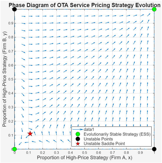
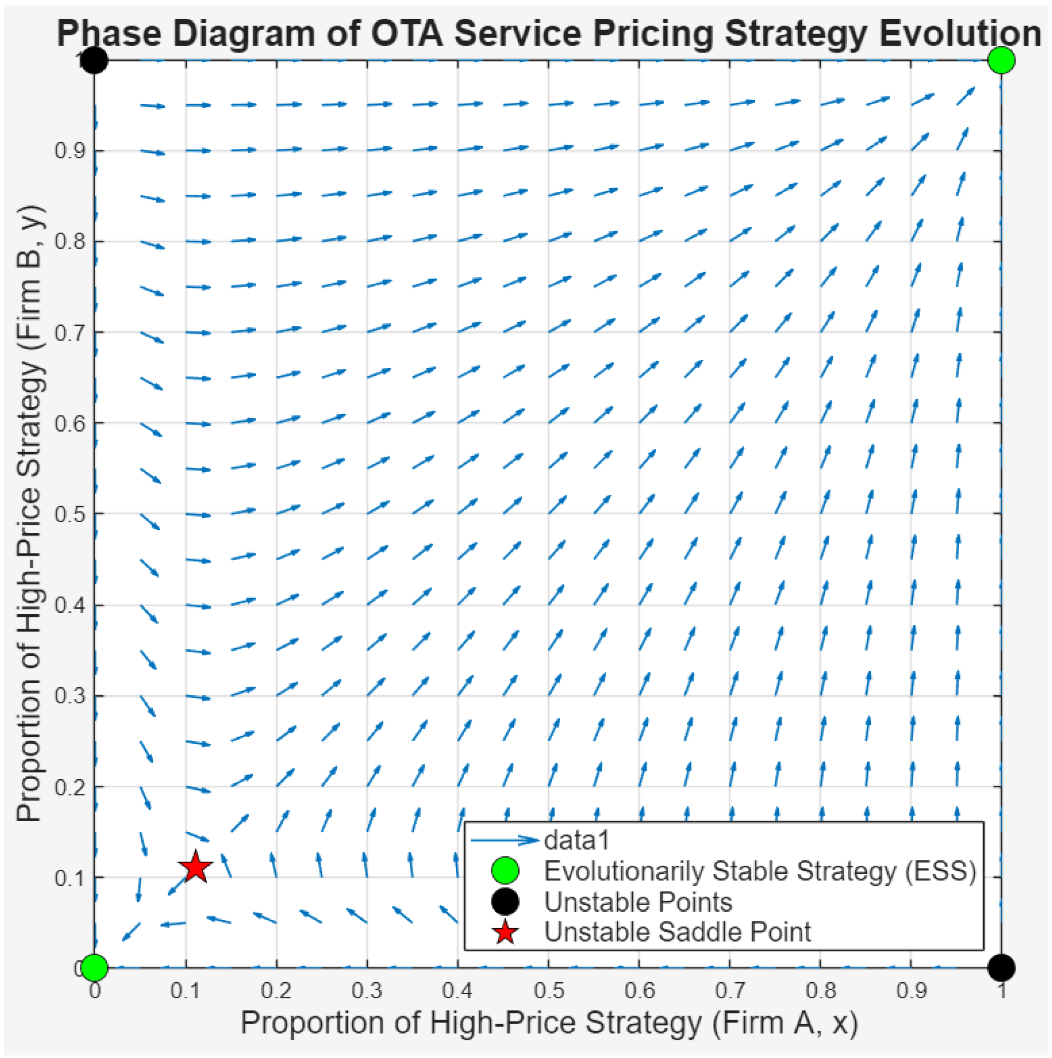
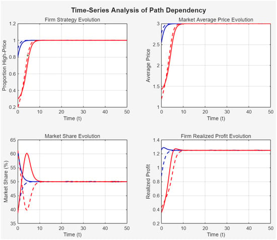
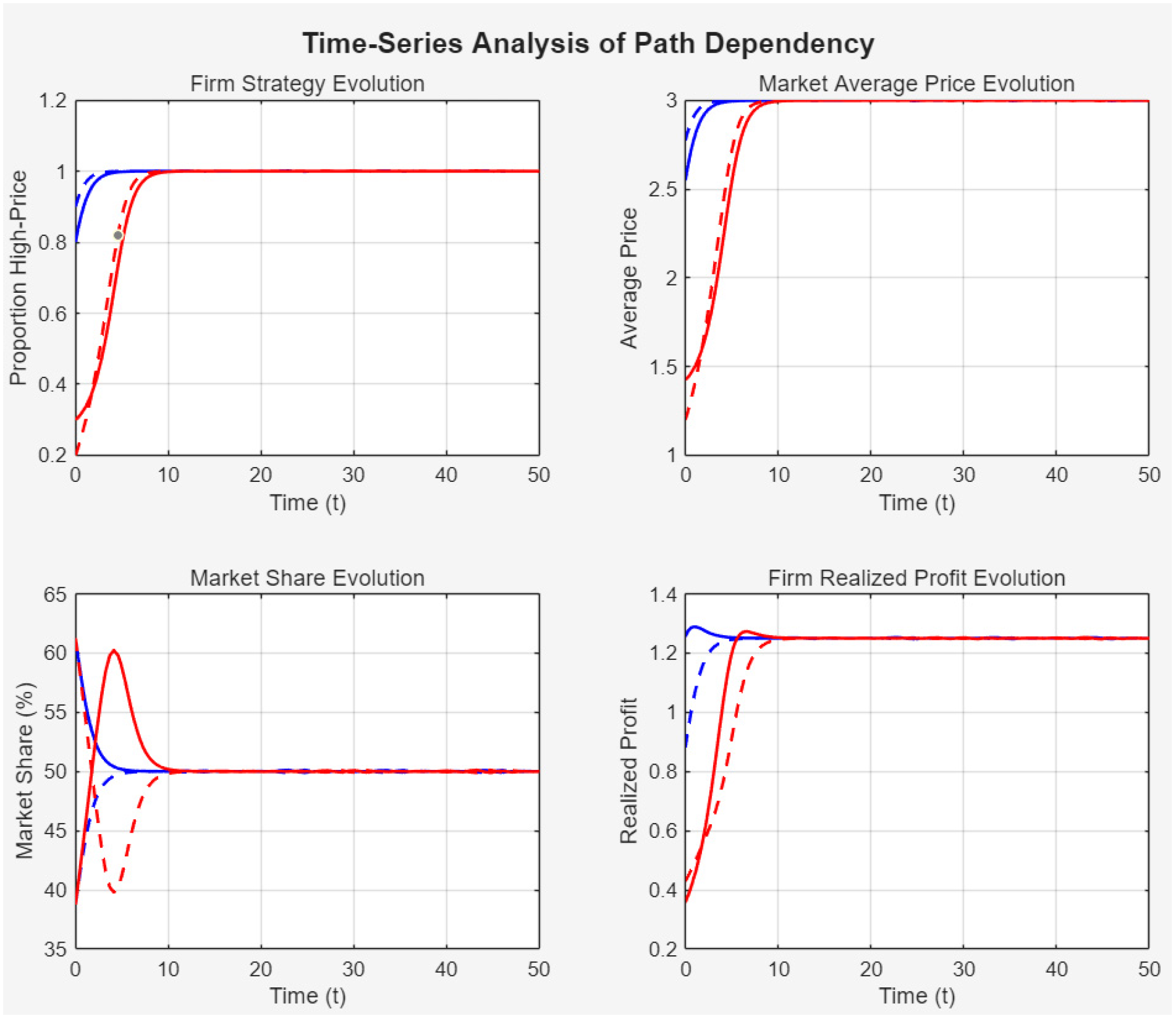
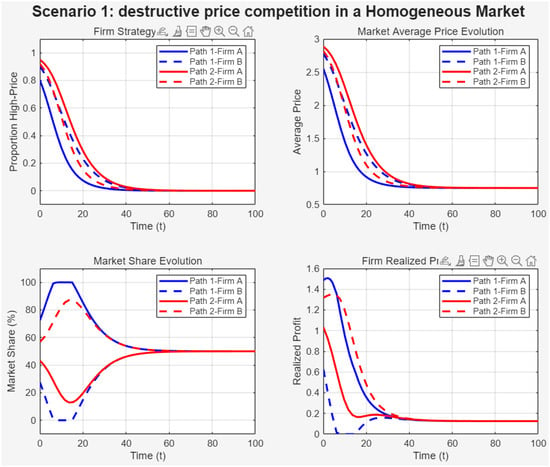
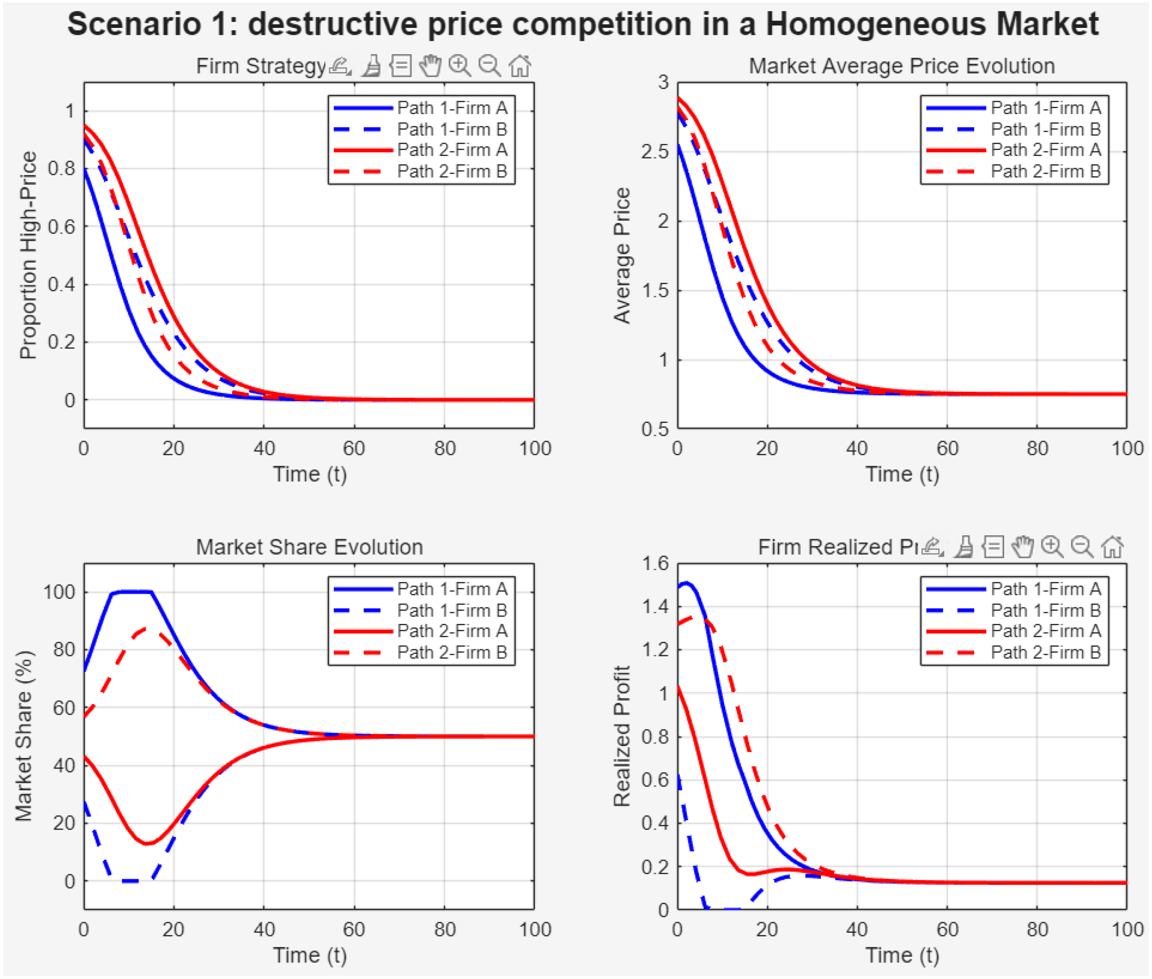
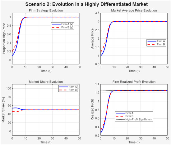
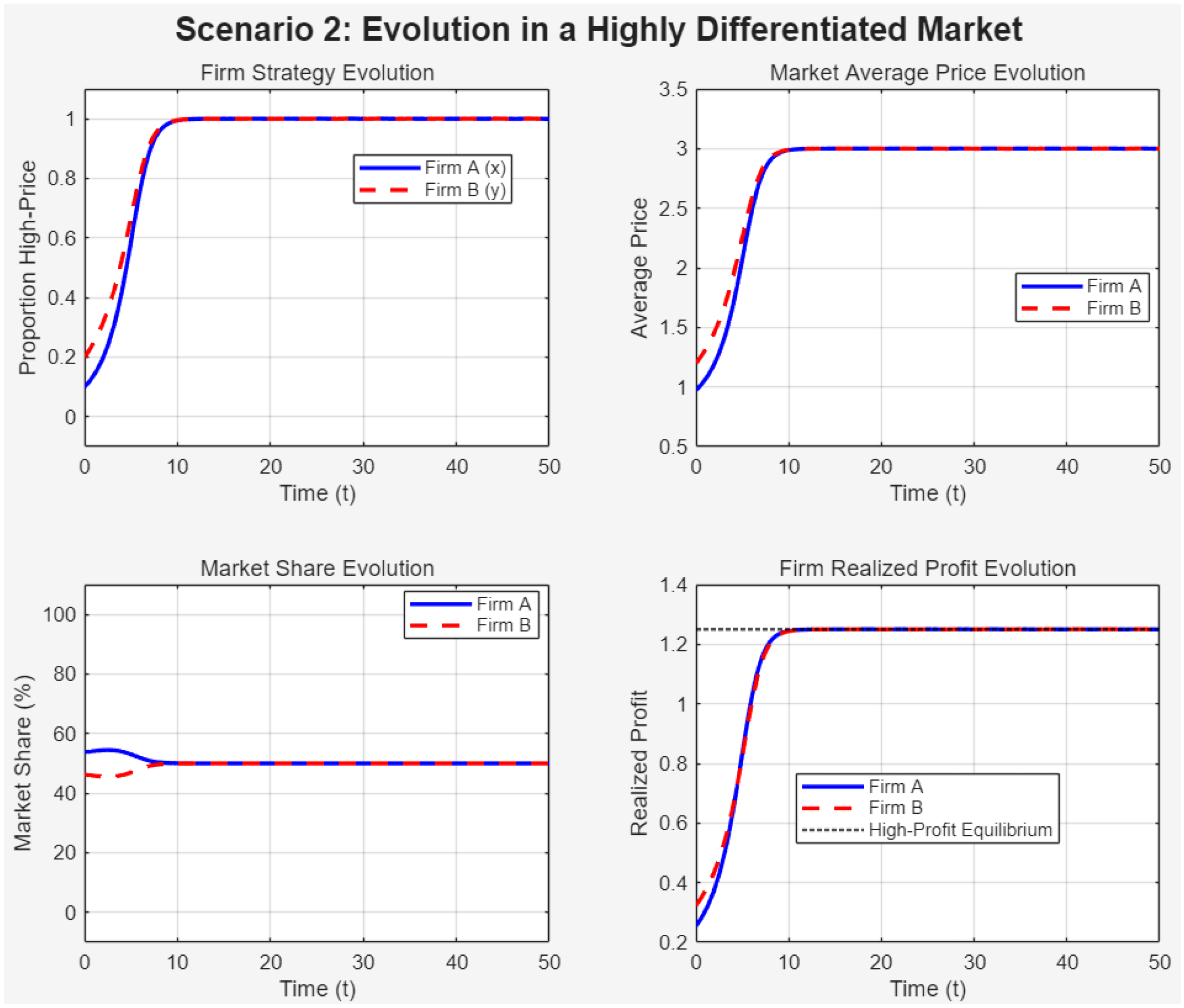
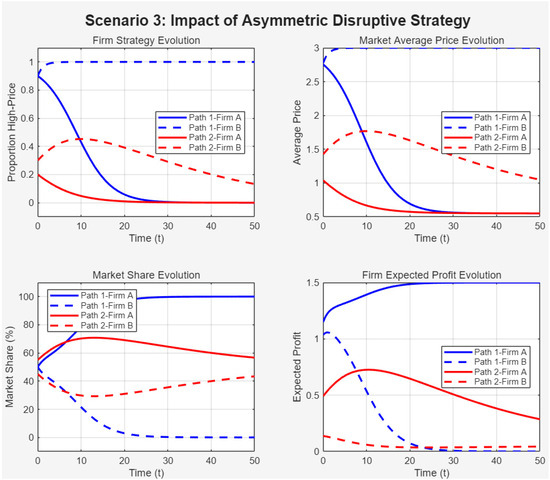
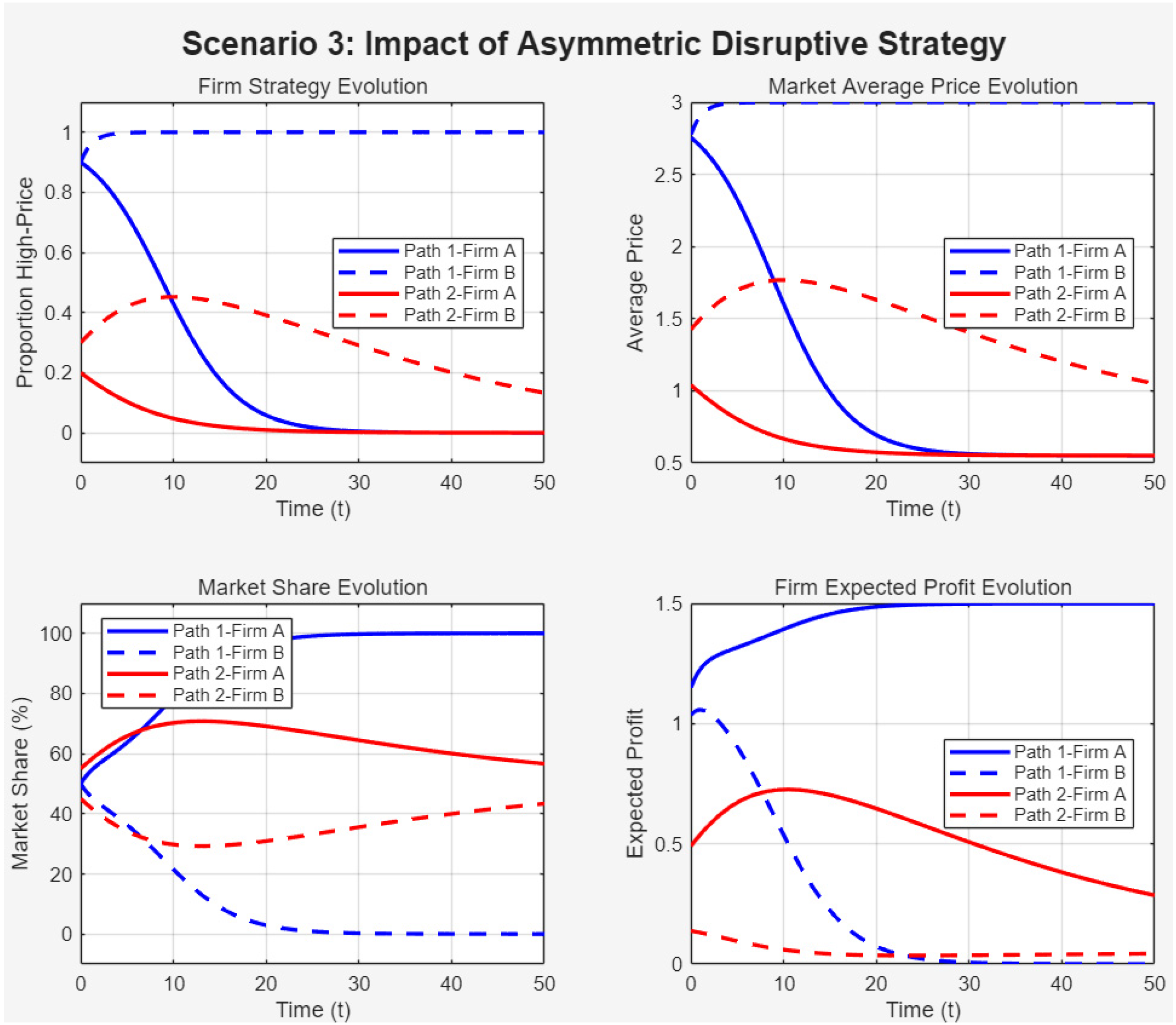
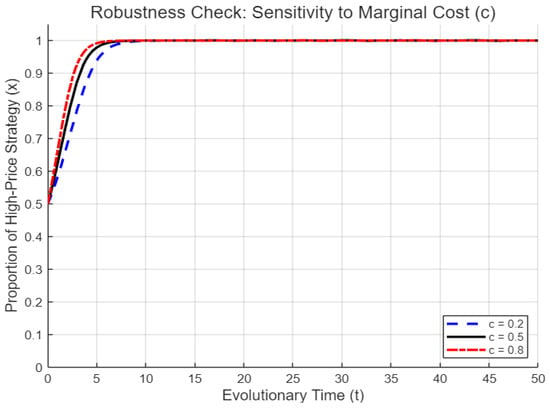
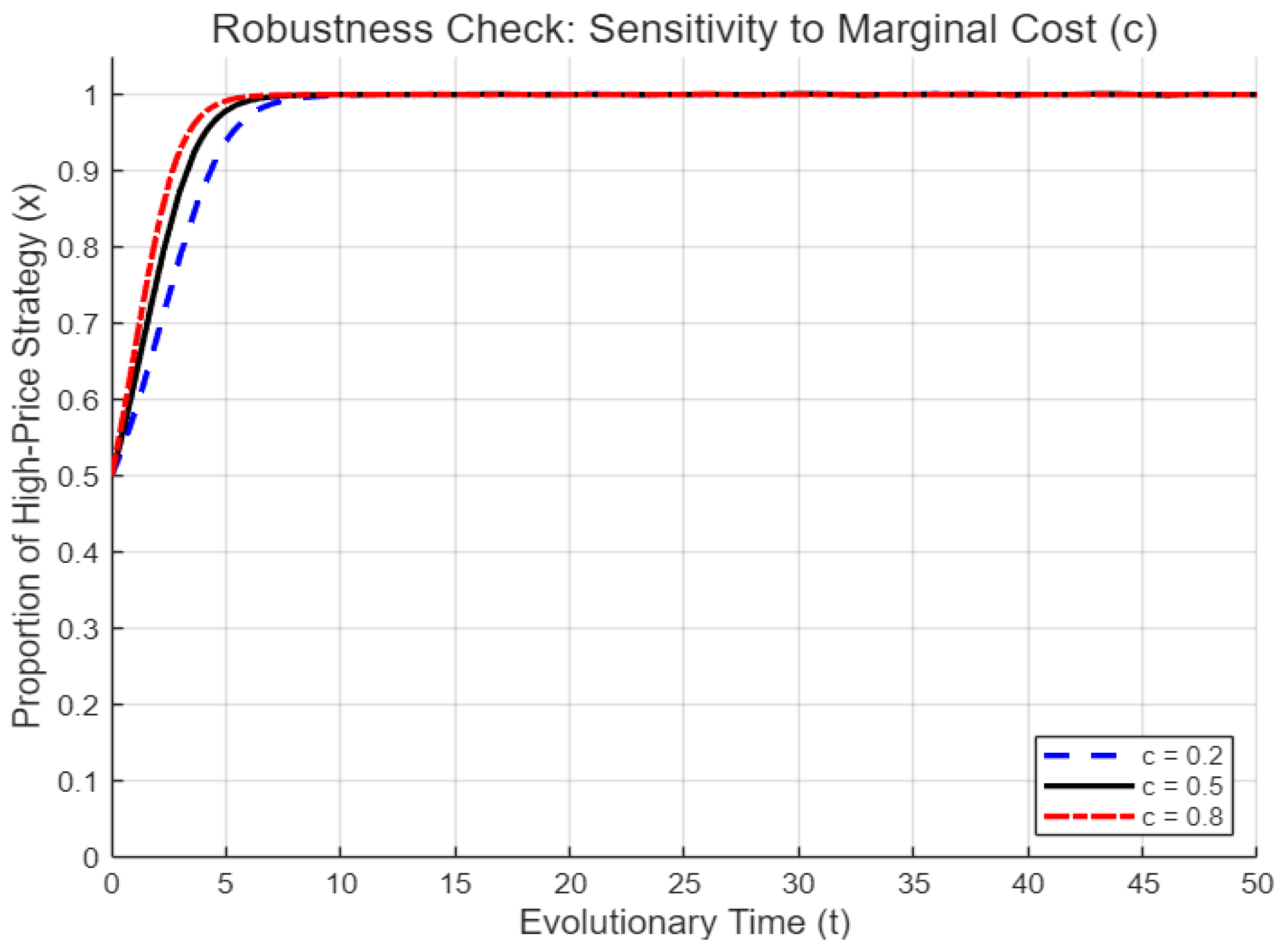
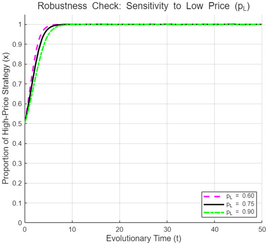

Disclaimer/Publisher’s Note: The statements, opinions and data contained in all publications are solely those of the individual author(s) and contributor(s) and not of MDPI and/or the editor(s). MDPI and/or the editor(s) disclaim responsibility for any injury to people or property resulting from any ideas, methods, instructions or products referred to in the content. |
© 2026 by the authors. Published by MDPI on behalf of the World Electric Vehicle Association. Licensee MDPI, Basel, Switzerland. This article is an open access article distributed under the terms and conditions of the Creative Commons Attribution (CC BY) license.