A Study on Self-Learning Energy Management Strategies for Personalized Driving in Plug-in Hybrid Electric Vehicles Based on Deep Reinforcement Learning

Abstract

To address the issue of reduced fuel efficiency in plug-in hybrid electric vehicles (PHEVs) caused by differences in driving styles, this paper proposes a personalized, self-learning energy management strategy (EMS) that integrates multi-feature driving style analysis with the Deep Deterministic Policy Gradient (DDPG). The study focuses on incorporating driving-style information into energy-management decisions. Firstly, based on CAN bus data, a Gaussian mixture model (GMM) is constructed using the expectation-maximization estimation method. By using weighted aggressive scores and preset thresholds, driving behaviors are classified into conservative, moderate, and aggressive types, thereby establishing personalized driving style representations. Second, a longitudinal dynamics model of the hybrid electric vehicle is established, incorporating the Pacejka tire model and a braking system model. Finally, a reward function is designed to minimize fuel consumption while penalizing excessively low battery state of charge (SOC). The driving-style code is included in the controller state, and DDPG jointly determines motor torque and the continuously variable transmission (CVT) ratio. Gaussian noise is added to the Actor output during training to explore the action space. A rule-based control strategy is adopted as a comparison strategy, and the proposed strategy is evaluated using the MATLAB (R2024b) platform. Over the 1980’s composite driving trajectory, equivalent fuel consumption decreases from 0.853 liters (L) to 0.705 L, a reduction of 17.34%. These results support the feasibility of the integrated strategy under the evaluated simulation conditions.

1. Introduction

As the energy crisis intensifies and environmental protection requirements continue to rise, the automotive industry is accelerating its transition toward electrification and intelligent technologies. Limited by factors such as battery energy density, charging infrastructure, and driving range, pure electric vehicles still face challenges in widespread adoption and application [1]. Plug-in hybrid electric vehicles (PHEVs) combine the extended driving range of conventional vehicles with the energy-efficiency and environmental benefits of electric vehicles and are considered an important technological approach to reducing transportation energy consumption and emissions [2]. As a core technology of PHEVs, the energy management strategy directly affects fuel economy, emissions, and vehicle performance [3]. However, real-world driving conditions are complex and uncertain, and differences in driver behavior and driving environments can lead to variations in vehicle energy consumption [4]. Analyzing driving behavior and incorporating driving-style information into energy management decisions are therefore important for improving fuel economy while adapting control decisions to individual driving characteristics [5].

Energy management strategies for hybrid vehicles have evolved from rule-based methods to optimization-based approaches [6]. Early studies primarily employed rule-based strategies, including logic-threshold and fuzzy-logic control [7,8]. These strategies have simple structures and are relatively easy to implement, but their control rules depend heavily on expert knowledge. They consequently have limited adaptability to unanticipated operating conditions and cannot guarantee global optimality [9]. Dynamic Programming (DP), as a typical global optimization method, can obtain a theoretically optimal solution and is therefore often used as a benchmark for evaluating other energy management strategies [10]. However, DP requires prior knowledge of the complete driving cycle and involves a heavy computational burden, which limits its direct application to real-time control systems. To balance optimization performance and real-time applicability, instantaneous and receding-horizon optimization methods, such as the Equivalent Consumption Minimization Strategy (ECMS) and Model Predictive Control (MPC), have been extensively investigated [11]. These methods generally rely on accurate system models, whereas hybrid electric vehicles are time-varying nonlinear systems whose dynamic characteristics are affected by coupled factors such as vehicle load, road gradient, and driving conditions [12].

With the development of connected-vehicle and big-data technologies, data-driven methods have become an important research direction in hybrid-vehicle energy management. Compared with conventional model-based approaches, data-driven methods can use vehicle operating data to characterize nonlinear system behavior and improve controller adaptation to complex operating conditions. He et al. [13] reviewed machine-learning approaches to hybrid electric vehicle energy management. Driving-behavior modeling and deep reinforcement learning (DRL) are two major research directions in this field. Previous studies have shown that driver operating habits can significantly affect vehicle energy consumption [14]. Identifying individual driver characteristics from driving data therefore provides an important basis for developing personalized energy management strategies [15]. Based on naturalistic driving data, He et al. [4] analyzed driving patterns using a hierarchical probabilistic model and K-means clustering and examined differences in driving style and energy consumption.

DRL has demonstrated considerable potential in vehicle energy management because it can address sequential decision-making problems and learn control policies through interactions with the vehicle environment [16]. Among DRL algorithms, the Deep Deterministic Policy Gradient (DDPG) is suitable for vehicle-control problems involving continuous action spaces [17]. Recent learning-based energy management studies have focused mainly on improving reinforcement-learning algorithms, incorporating driving-condition information, and enhancing controller generalization. Wu et al. [18] applied the Twin Delayed Deep Deterministic Policy Gradient (TD3) algorithm to charge-sustaining control for a multi-mode PHEV. Zhang et al. [19] employed Proximal Policy Optimization (PPO) to account for battery thermal characteristics. Huang et al. [20] investigated transfer reinforcement learning to improve the transferability of energy management policies across different hybrid-electric-vehicle platforms. More recent studies have incorporated driving-condition recognition into TD3-based energy management [21] and improved Soft Actor-Critic (SAC) using prioritized experience replay and curriculum learning [22]. These studies mainly address learning performance, battery thermal characteristics, vehicle-platform transfer, and driving-condition adaptability.

Driving-style-aware energy management methods have also received increasing attention. Zhu et al. [23] considered driving-style uncertainty in personalized eco-adaptive cruise control, while Shao et al. [15] incorporated driving-cycle recognition into predictive energy management. Wang et al. [24] combined driving-style recognition with MPC and adaptive ECMS for plug-in hybrid buses and evaluated the method through simulation and hardware-in-the-loop testing. These studies demonstrate the relevance of driver- and condition-related information to energy management decisions. However, limited attention has been given to integrating a driving-style representation derived from CAN data into the state of a DRL controller for the joint continuous control of motor torque and the continuously variable transmission (CVT) ratio.

Table 1. (a) Comparison of Representative Energy Management Studies: Methods and Information Inputs. (b) Comparison of Representative Energy Management Studies: Evaluation, Contributions, and Research Gaps.

(a)
Study	Vehicle	Strategy	Driving Data	Condition Input	State
[7]	PHEV	Fuzzy logic	Operating data	-	Demand and SOC
[11]	PHEV bus	ECMS-MPC	Predicted demand	Thermal	SOC and thermal states
[15]	PHEV	Predictive EMS	Recognized driving cycle	Cycle class	Cycle and vehicle state
[18]	Multi-mode PHEV	TD3	Driving cycle	-	Continuous states
[19]	PHEV bus	PPO	Battery thermal state	Thermal condition	Powertrain and thermal states
[21]	PHEV	TD3	Recognized condition	Condition-aware	State plus condition
[22]	Hybrid bus	SAC	Multimodal cycles	-	State and mode
[23]	PHEV	Co-optimization	Car following data	Driving style uncertainty	Speed, spacing, and power
[24]	PHEV bus	MPC + AECMS	Car following and style	Driving style	Style, traffic, and SOC
This study	PHEV	DDPG	33 CAN segments	Ordinal driving-style code	Six-dimensional state
(b)
Study	Objective	Benchmark	Validation	Contribution	Gap
[7]	Energy use	Conventional strategy	Simulation	Fuzzy EMS	Expert-rule dependence; no learned continuous policy
[11]	Economy and temperature	Conventional EMS	Simulation	Thermal-aware predictive EMS	Model- and prediction-dependent
[15]	Fuel economy	Fixed-cycle EMS	Simulation	Cycle adaptation	No driver-specific style code
[18]	Fuel use and SOC	DDPG	Simulation	Improved learning stability	No driving-style code
[19]	Fuel use and thermal state	Conventional EMS	Simulation	Thermal-aware policy	No driver-style input
[21]	Fuel economy	TD3	Simulation	Condition adaptation	Driver style not isolated
[22]	Fuel use and learning	SAC	Simulation	Learning-efficiency enhancement	No driver-style input
[23]	Economy and tracking	Eco-ACC baseline	Simulation	Personalized co-optimization	Not CAN-style DRL or joint CVT control
[24]	Fuel economy	Conventional EMS	Simulation and HIL	Closest style-aware comparator	Not DRL; no joint motor-torque
This study	Equivalent fuel and SOC	Rule-based strategy	Simulation	CAN style + continuous joint control	One composite trajectory; no matched RL baselines

shows that recent TD3, PPO, transfer-learning, and SAC studies primarily address learning stability, thermal management, platform transfer, or driving-condition adaptation. Reference [24] is the closest style-aware comparator, but it combines MPC with adaptive ECMS and does not learn the joint motor-torque and CVT-ratio action used here. Accordingly, the specific research gap addressed in this study is the integration of a CAN-derived ordinal driving-style code into a DDPG state for joint continuous PHEV control.

To address this research gap, the primary objective of this study is to develop and evaluate a personalized, self-learning EMS that uses a CAN-derived driving-style representation as an explicit input to a continuous-control PHEV controller. To achieve this objective, the proposed framework integrates multi-feature driving-style analysis with DDPG and jointly determines motor torque and the CVT ratio. The main contributions of this study are as follows:

(1) A personalized driving-style identification procedure is developed using eight driving-behavior features extracted from CAN data. The features are standardized and clustered using a Gaussian mixture model whose parameters are estimated through the Expectation-Maximization algorithm. A weighted aggressiveness score and threshold classification are subsequently used to identify conservative, moderate, and aggressive driving styles.

(2) The identified driving-style code is incorporated into the six-dimensional state of a DDPG energy management controller. The controller jointly determines motor torque and the CVT ratio through a two-dimensional continuous action, thereby linking personalized driving information with continuous PHEV powertrain control.

The remainder of this paper is organized as follows. Section 2 presents the PHEV component models, the CAN-data-based driving-style classification method, the personalized controller-state construction, and the DDPG energy management strategy. Section 3 describes the simulation setup and analyzes the simulation results. Section 4 compares the proposed approach with related energy management strategies and discusses the limitations and directions for future work. Section 5 presents the conclusions.

2. PHEV Modeling and Personalized Energy Management Strategy Development

As complex systems that combine both an internal combustion engine and an electric motor as power sources, hybrid vehicles feature strong power coupling and frequent changes in operating conditions, which place high demands on the accuracy of vehicle modeling. This section focuses on modeling methods for key components of hybrid vehicles, with the aim of developing a vehicle-level model that accurately reflects the actual operating characteristics of the vehicle.

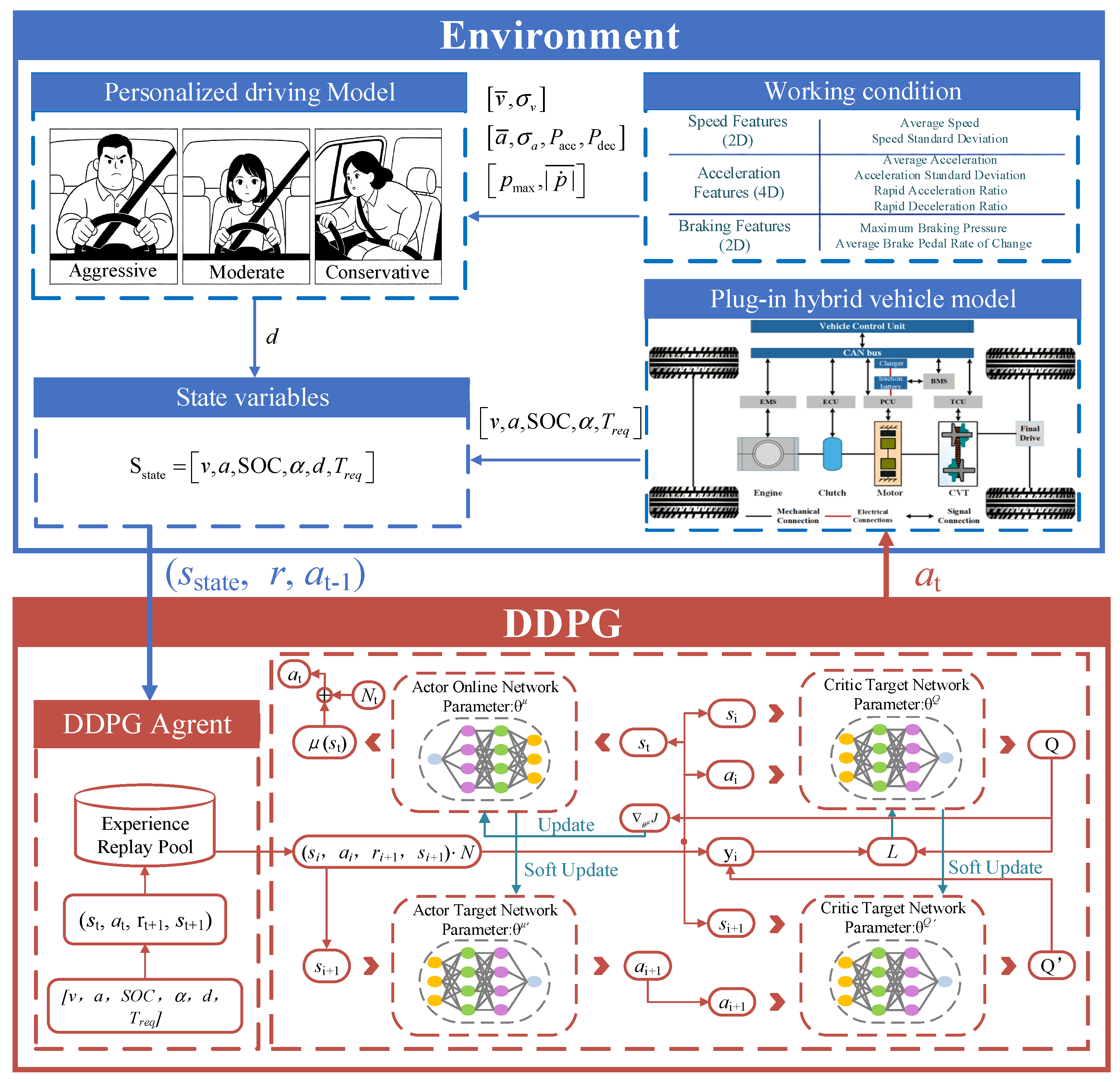
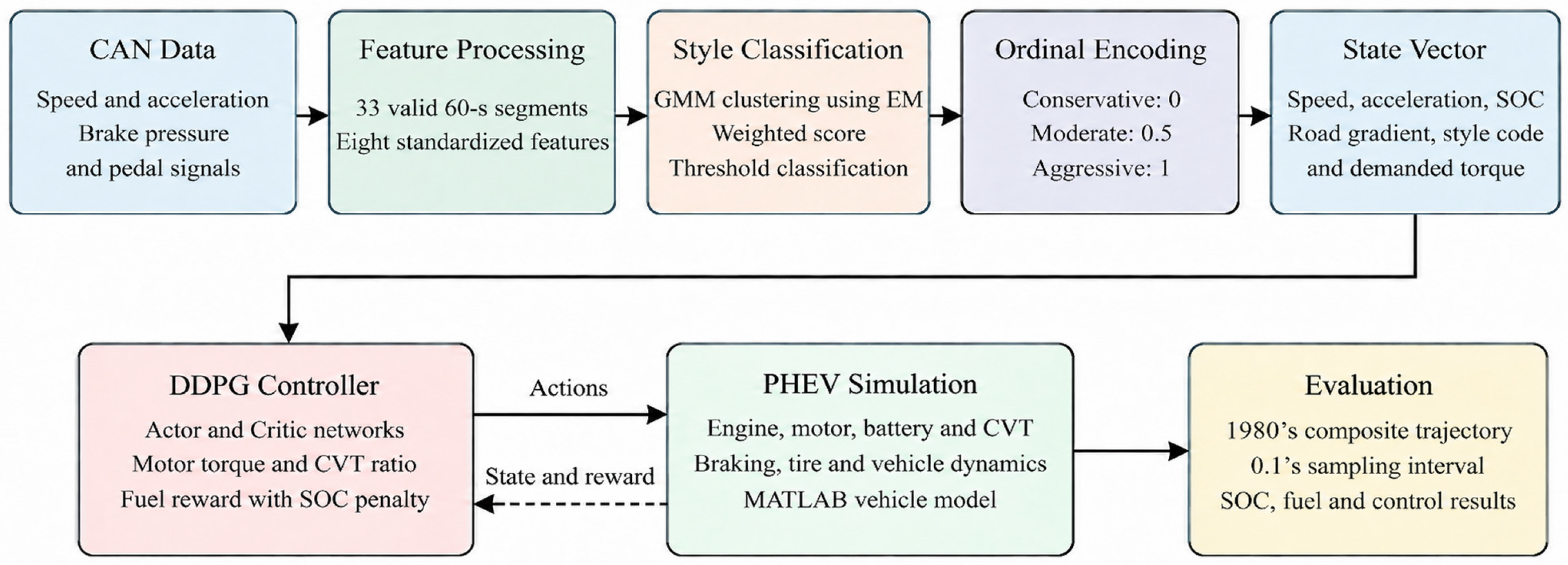
The overall framework of the research is shown in Figure 1.

2.1. Plug-in Hybrid Electric Vehicle Architecture

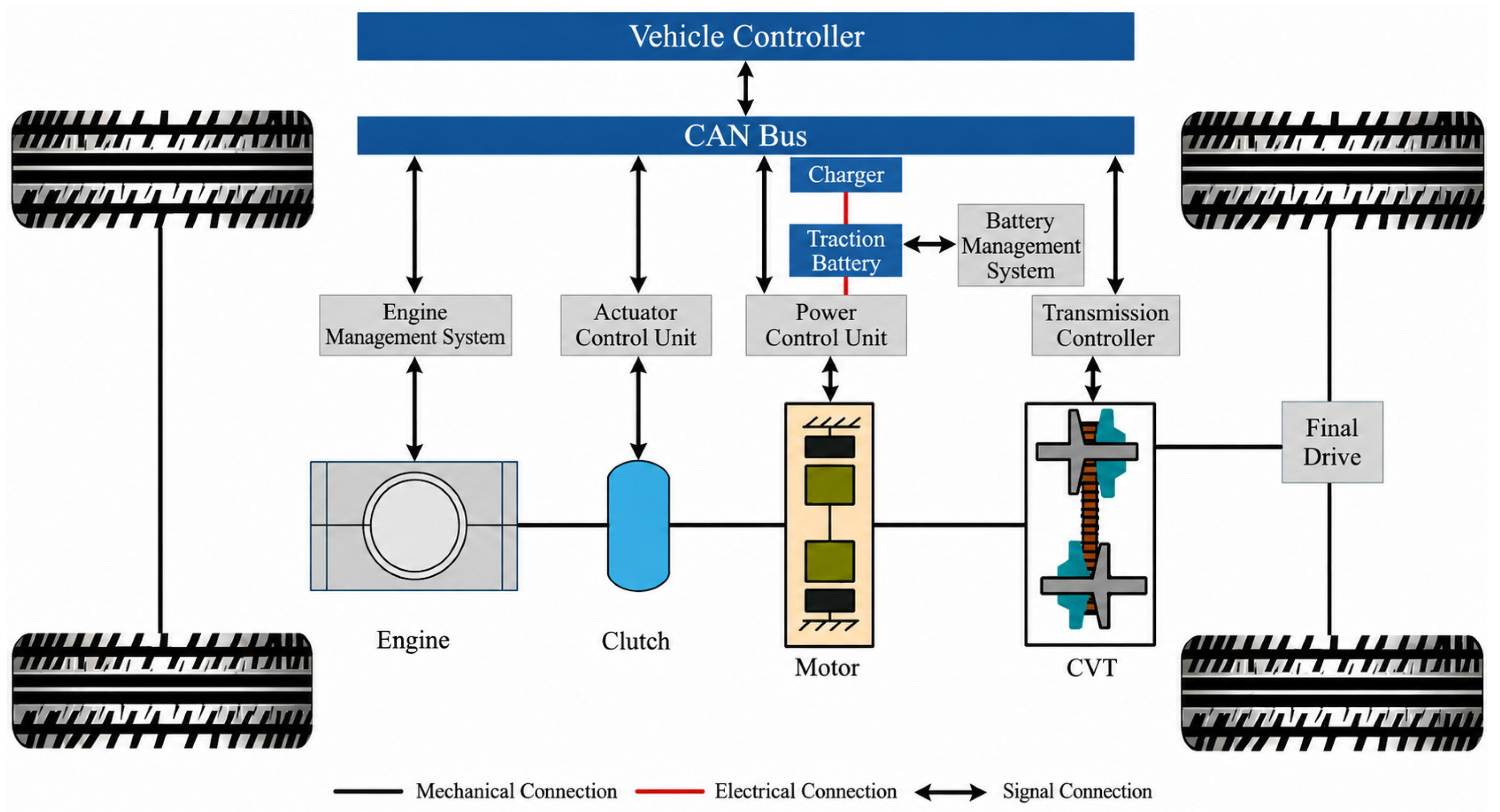
This paper focuses on plug-in hybrid electric vehicles, whose architecture is shown in Figure 2. The system consists primarily of core components such as the engine, electric motor, vehicle control unit, continuously variable transmission (CVT), power battery, and clutch. The internal combustion engine and the electric motor are integrated via the vehicle control unit, allowing them to power the vehicle either independently or in combination. The system can switch between operating modes—such as all-electric drive, hybrid drive, in-motion charging, and regenerative braking—based on the vehicle’s operating status. The vehicle control unit integrates information such as driver input, vehicle status, and SOC to make real-time decisions regarding operating modes and torque distribution, thereby achieving a balanced optimization of the vehicle’s performance and fuel efficiency.

2.2. Hybrid Vehicle Component and Longitudinal-Dynamics Models

This section describes the vehicle dynamics and the energy conversion among various components through the establishment of a mathematical model, and evaluates the energy management strategy through simulation. The following subsections present the engine, electric motor, power battery, drivetrain, braking system, tire, and longitudinal-dynamics models.

2.2.1. Engine Model

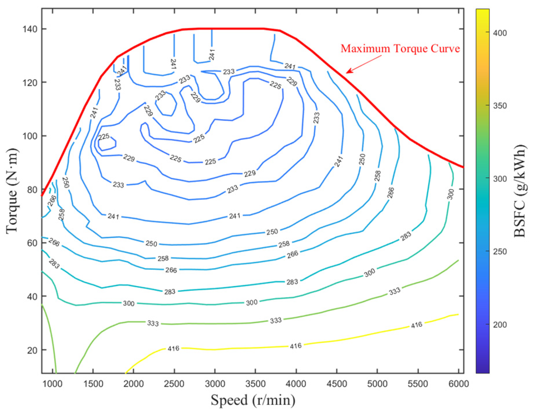
The engine is one of the main power sources in a hybrid vehicle, and its fuel economy directly affects the vehicle’s overall energy consumption [25]. A numerical engine model is developed from engine test-bench data. Fuel-consumption rates at different speeds and torques are obtained through interpolation and lookup tables [26]. The engine characteristics are shown in Figure 3.

The effective engine power is calculated as follows [26]:

$$P_e={\displaystyle \frac{n_e{T}_e}{9550}}$$

(1)

In the equation, P_e refers to the engine output power, kW; n_e represents the engine speed, r/min; T_e represents engine torque, N∙m; and b_e represents effective fuel consumption rate, g/(kw∙h).

The instantaneous engine fuel consumption ${\dot{m}}_f$ (g/s) is:

$${\dot{m}}_f={\displaystyle \frac{b_e{P}_e}{3600}}$$

(2)

The engine’s operating range is limited by its external characteristics; its maximum torque varies with engine speed, and the minimum torque is typically defined as the idle torque.

2.2.2. Electric Motor Model

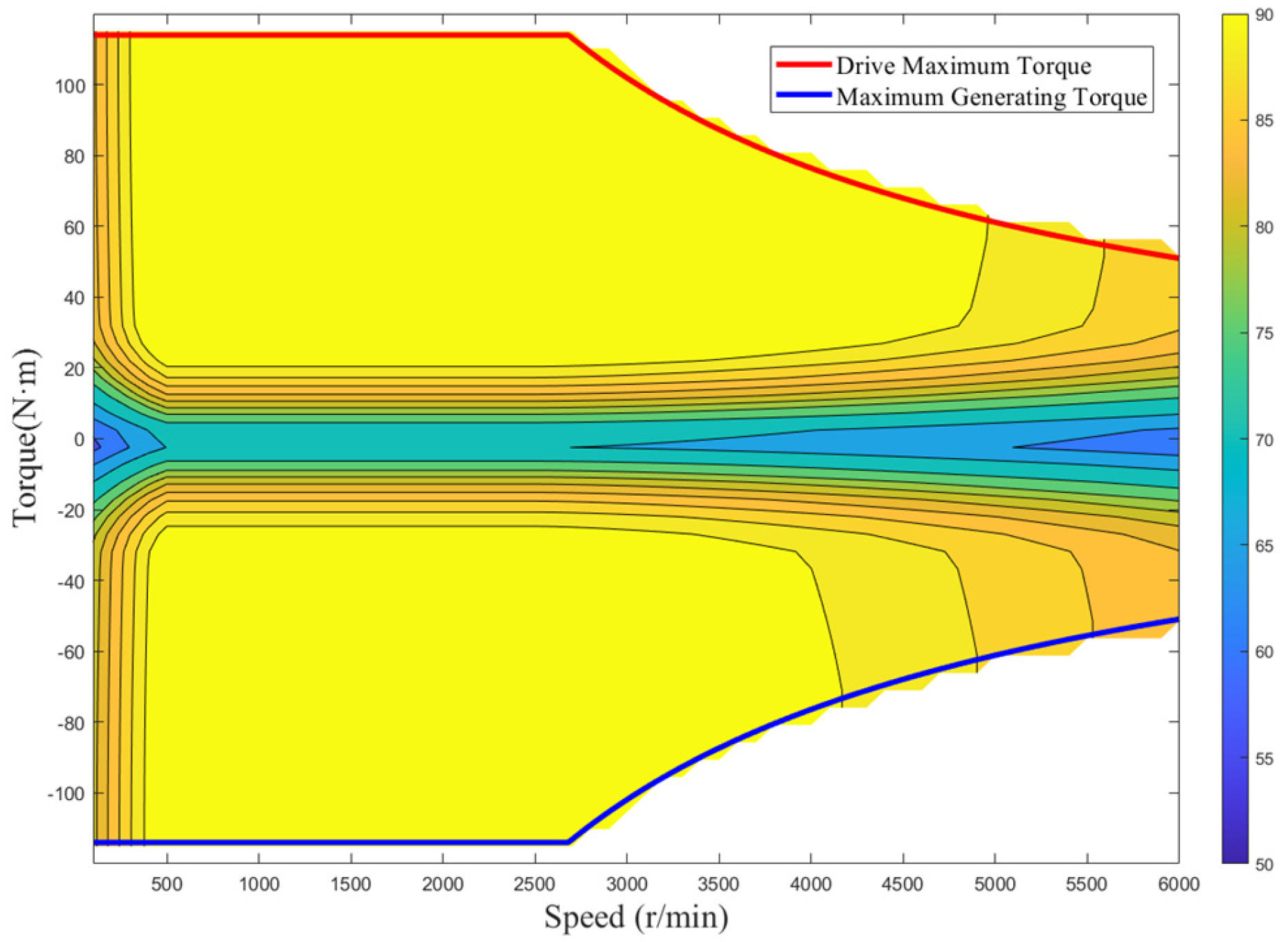
The selected motor is a permanent-magnet synchronous motor (PMSM). It can operate in motor and generator modes and provides constant torque at low speed and constant power at high speed. The motor model was developed using numerical modeling methods. Based on the test data of motor efficiency, the interpolation method was employed to determine the motor efficiency under different rotational speeds and torques [27]. The motor efficiency curve is shown in Figure 4.

The relationship between motor power, speed, and torque is as follows [27]:

$$P_m={\displaystyle \frac{n_m{T}_m}{9550}}$$

(3)

In the equation, P_m represents the mechanical power of the motor, in kW;

n_m represents the motor speed, in r/min; and T_m represents the motor torque, in N·m.

Motor efficiency satisfies:

η_m = f_m(n_m,T_m)

(4)

Motor Input/Output Electrical Power P_m,elec is related to mechanical power as follows:

$$P_{m,\mathit{elec}}=\left\{\begin{array}{ll}{\displaystyle \frac{P_m}{{\eta }_m}},\hfill & T_m\ge 0\hspace{1em}\hfill \\ P_m{\eta }_m,\hfill & T_m<0\hfill \end{array}\right.$$

(5)

2.2.3. Power Battery Model

Power batteries serve as energy storage devices in hybrid vehicles. This study uses an internal resistance model to describe the dynamic characteristics of the battery [28]. This model represents the battery pack as a circuit consisting of an ideal voltage source in series with an internal resistance. According to Ohm’s law, the terminal voltage of the battery is:

U_b = E_o − I_bR_o

(6)

In the equation, U_b represents the battery terminal voltage, V; E_o represents the open-circuit voltage of the battery, V; I_b represents the battery current, A; and R_o is the battery’s internal resistance, Ω.

The SOC is estimated using the ampere-hour integration method, taking into account the effects of charging and discharging efficiencies:

$$S_{\mathrm{soc}}(t)=S_{\mathrm{soc},0}-{\displaystyle \frac{{\displaystyle {\int }_{t_0}^t{I}_b}(t)\mathit{dt}}{3600C}}$$

(7)

In the equation, C represents the battery’s rated capacity, A·h; S_soc,0 is the initial SOC value.

The battery power requirement P_bat is related to the electrical power required P_m,elec by the motor as follows:

$$P_{\mathit{bat}}=\left\{\begin{array}{ll}{\displaystyle \frac{P_{m,\mathit{elec}}}{{\eta }_{\mathit{bat},\mathit{dis}}}},\hfill & P_{m,\mathit{elec}}\ge 0\hspace{1em}\hfill \\ P_{m,\mathit{elec}}{\eta }_{\mathit{bat},\mathit{chg}},\hfill & P_{m,\mathit{elec}}<0\hfill \end{array}\right.$$

(8)

In the equation, η_bat,dis and η_bat,chg represent the battery’s discharge and charge efficiencies, respectively.

2.2.4. Drivetrain Model

The drivetrain is the key component that transmits power from the engine and electric motor to the wheels. The torque output from the engine and electric motor is transmitted to the CVT via a coupling. It is then transmitted through the main reduction gear to the drive wheels. To simplify the modeling, this paper ignores nonlinear factors such as torsional vibration and backlash in the drive shaft, focusing instead on the relationship between torque and rotational speed.

The required torque at the input end of the torque coupler consists of both the engine’s required torque and the motor’s required torque [29]:

T_req = T_e,req + T_m,req

(9)

In the equation, T_req represents the total required torque at the coupler’s input end, N·m; T_e,req represents the engine’s required torque, N·m; and T_m,req represents the required torque of the motor, N·m.

The relationship between the torque at the drive wheel and the required torque at the input end of the torque coupler is as follows:

$$T_{\mathit{req}}={\displaystyle \frac{T_w}{i_{\mathit{CVT}}{i}_T{\eta }_{\mathit{CVT}}{\eta }_T{\eta }_0}}$$

(10)

In the equation, T_w represents the drive torque at the drive wheel, in N·m; i_CVT represents the CVT gear ratio; i_T represents the final drive ratio; η_CVT represents the CVT transmission efficiency; η_T represents the final drive efficiency; and η₀ represents the torque converter efficiency.

The relationship between rotational speeds is as follows:

$$\left\{\begin{array}{l}{n}_{\mathit{req}}=n_w{i}_{\mathit{CVT}}{i}_T\hfill \\ n_{\mathit{req}}=n_e=n_m\hfill \end{array}\right.$$

(11)

In the equation, n_w represents the rotational speed of the drive wheel, in r/min; n_req represents the rotational speed at the input end of the coupler, in r/min.

The relationship between the drive wheel speed and vehicle speed is as follows:

$$n_w={\displaystyle \frac{v}{0.377r}}$$

(12)

In the equation, v is the vehicle speed, in km/h; r is the wheel radius, in m.

2.2.5. Braking-System Model

The braking system model takes into account the coordination between hydraulic braking and regenerative braking. The relationship between the total braking torque and the braking pressure is as follows:

T_b = η_b ⋅ p_b

(13)

In the equation, T_b represents the total braking torque, in N·m; p_b represents the braking pressure, in bar; and η_b represents the braking efficiency coefficient.

2.2.6. Tire Model

This study uses Pacejka’s “Magic Formula” tire model to calculate the longitudinal force on the drive wheels [30]. The formula for calculating the longitudinal force is:

$$\left\{\begin{array}{l}{F}_x(\kappa )=D_x\sin [C_x\arctan (B_x\kappa -E_x(B_x\kappa -\arctan (B_x\kappa )))]\hfill \\ F_{x,\mathit{max}}=\mu \cdot \mathit{Fz}\hfill \end{array}\right.$$

(14)

In the equation, F_x represents the longitudinal force, in N; κ represents the longitudinal slip rate; D_x, C_x, B_x, and E_x are fitting parameters; μ represents the road surface coefficient of friction; and F_z represents the normal load on the drive wheel, in N.

2.2.7. Longitudinal-Dynamics Model

Vehicle longitudinal dynamics describe the relationship between the external forces acting on a vehicle during motion and its state of motion [29]. If we neglect the vehicle’s lateral and vertical motion and consider only longitudinal forces, the equation of motion for the vehicle is:

F_t = F_f + F_w + F_i + F_j

(15)

In the equation, F_t represents the driving force, in N; F_f represents rolling resistance, in N; F_w represents air resistance, in N; F_i represents gradient resistance, in N; and F_j represents acceleration resistance, in N.

Expanding the various resistances, Equation (15) can be written as:

$${\displaystyle \frac{T_w}{r}}=\mathit{fm} \mathit{g}+{\displaystyle \frac{C_{D}A{v}^2}{21.15}}+\mathit{mg}\sin \mathit{\alpha }+\mathit{\delta m}{\displaystyle \frac{\mathit{dv}}{\mathit{dt}}}$$

(16)

In the equation, m is the vehicle mass, in kg; g is the acceleration due to gravity, in m/s²; f is the rolling resistance coefficient; α is the road gradient, in degrees; C_D is the drag coefficient; A is the frontal area, in m²; and δ is the rotational mass conversion factor.

2.3. Vehicle Simulation Model

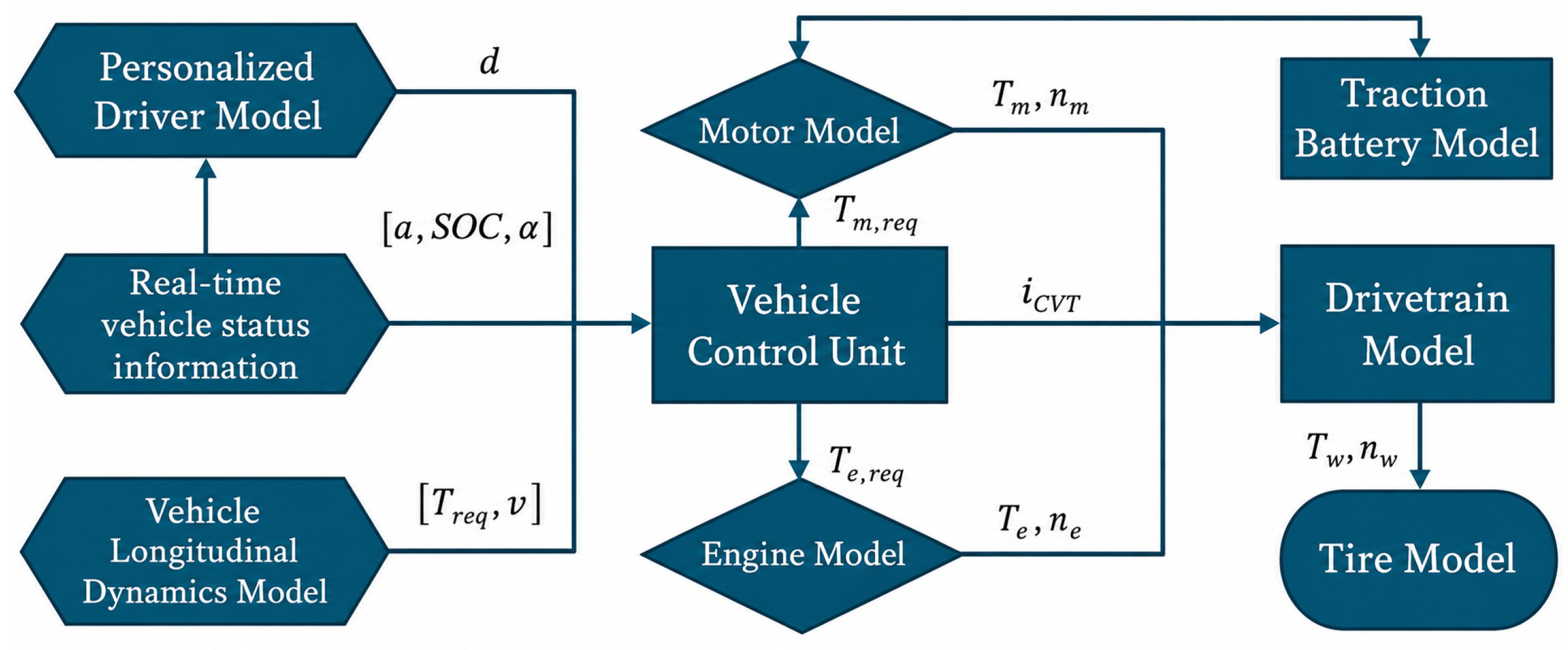
Based on the above submodels, a full-vehicle simulation model was developed in MATLAB, as shown in Figure 5.

The vehicle model takes the personalized driver model, vehicle operating status, and longitudinal-dynamics model as inputs. The personalized driver model determines the driving style and outputs the ordinal style code defined in Section 2.4.3.

At the same time, real-time vehicle information provides acceleration, SOC, and road gradient, while the longitudinal-dynamics model calculates demanded torque and vehicle speed. These signals are fed to the controller, which determines engine torque, target motor torque, and the CVT ratio. The engine and motor models then produce the corresponding torque and speed, and the drivetrain transfers the coupled power to the wheels.

The parameters of the main components of the plug-in hybrid electric vehicle studied in this paper are shown in

Table 2. Key Component Specifications for the Plug-in Hybrid Electric Vehicle.

	Parameters	Value
Basic Specifications	Total mass (kg)	1580
	Frontal area (m2)	2.38
	Wheel radius (m)	0.289
	Rolling resistance coefficient	0.0083
	Drag coefficient (dimensionless)	0.357
Engine	Rated power (kW)	93
	Maximum torque (N·m)	140
	Speed range (r/min)	800–6000
Motor	Rated power (kW)	32
	Maximum torque (N·m)	114
	Speed range (r/min)	0–6000
Power Batteries	Rated capacity (A·h)	40
	Rated voltage (V)	352
	SOC operating range	0.3–0.9
Drivetrain	CVT ratio range	0.422–2.432
	Final-drive ratio	5.297
	Drivetrain efficiency	0.92

.

2.4. Driving-Style Classification and Personalized State Construction

The performance of energy management strategies for hybrid vehicles depends not only on the vehicle’s own dynamic characteristics but is also influenced by the driver’s behavior. Different drivers exhibit differences in acceleration, braking, and speed selection, which affect energy consumption. This section first extracts and standardizes multidimensional driving behavior features based on CAN data. A Gaussian mixture model estimated using Expectation-Maximization identifies three clusters. Weighted scoring and threshold classification are then used to label the clusters as conservative, moderate, and aggressive. The resulting style code is incorporated into the state space of the DDPG energy-management controller.

2.4.1. Driving-Behavior Feature Extraction

To characterize driving behavior, this section extracts eight driving-behavior features from CAN data. The available dataset contains 33 valid 60’s driving segments. For each segment, the following speed, acceleration, and braking features are calculated:

Speed Characteristics (2-D): Average Speed $\overline{v}$, Speed Standard Deviation σ_v.

Acceleration Characteristics (4-D): Average acceleration a, standard deviation of acceleration σ_a, proportion of rapid acceleration P_acc (proportion of samples with acceleration above 1.5 m·s⁻²), and proportion of rapid deceleration P_dec (proportion of samples with acceleration below −2.0 m·s⁻²).

Braking Characteristics (2-D): Maximum braking pressure and mean absolute rate of change of braking pressure, as defined in Equations (16) and (17).

The eight features are defined as follows:

$$\left\{\begin{array}{l}{f}_1=\overline{v}={\displaystyle \frac{1}{N}}{\displaystyle \sum _{i=1}^N{v}_i}, f_2={\sigma }_v=\sqrt{{\displaystyle \frac{1}{N-1}}{\displaystyle \sum _{i=1}^N{(v_i-\overline{v})}^2}}\\ f_3=\overline{a}={\displaystyle \frac{1}{N}}{\displaystyle \sum _{i=1}^N{a}_i}, f_4={\sigma }_a=\sqrt{{\displaystyle \frac{1}{N-1}}{\displaystyle \sum _{i=1}^N{(a_i-\overline{a})}^2}}\\ f_5=P_{\mathrm{acc}}={\displaystyle \frac{\{a_i>1.5\}}{N}}, f_6=P_{\mathrm{dec}}={\displaystyle \frac{\{a_i<-2.0\}}{N}}\\ f_7=p_{\max }={\max }_{1\le i\le N}{p}_i, f_8=\overline{\left|\dot{p}\right|}={\displaystyle \frac{1}{N-1}}{\displaystyle \sum _{i=1}^{N-1}\frac{|p_{i+1}-p_i|}{\Delta t}}\end{array}\right.$$

(17)

In this equation, N represents the number of sampling points within a segment, and ${\dot{P}}_b$ represents the first-order differential approximation of the braking pressure.

2.4.2. Feature Standardization and Driving-Style Classification

In Section 2.4.1, a feature vector is constructed for each driving segment from the eight behavior features:

$$f={\left[\overline{v},{\sigma }_v,\overline{a},{\sigma }_a,P_{\mathrm{acc}},P_{\mathrm{dec}},p_{\max },\overline{\left|\dot{p}\right|}\right]}^T$$

(18)

To avoid differences in units and scale, the feature matrix is standardized as follows:

$$\left\{\begin{array}{l}{\mu }_j={\displaystyle \frac{1}{M}}{\displaystyle \sum _{i=1}^M{f}_{\mathit{ij}}}\\ {\sigma }_j=\sqrt{{\displaystyle \frac{1}{M-1}}{\displaystyle \sum _{i=1}^M{(f_{\mathit{ij}}-{\mu }_j)}^2}}\\ {\tilde{f}}_{\mathit{ij}}={\displaystyle \frac{f_{\mathit{ij}}-{\mu }_j}{{\sigma }_j}}\end{array}\right.$$

(19)

In Equation (19), M represents the total number of valid driving segments; f_ij represents the value of feature j in driving segment i; μ_j and σ_j are the mean and standard deviation of feature j, respectively. The standardized feature is obtained by subtracting its mean and dividing by its standard deviation. This scaling reduces differences arising from feature units and numerical magnitudes.

For the three driving-style categories, Equation (20) expresses a probability density as a weighted sum of three Gaussian components [4]. In this expression, π_k is the mixture weight of component k, μ_k is its mean vector, and Σ_k is its covariance matrix; the nonnegative weights sum to one.

$$P(\tilde{f}|\theta )={\displaystyle \sum _{k=1}^3{\pi }_k}\mathcal{N}\left(\tilde{f}\mid {\mu }_k,{\sum }_k\right)$$

(20)

The model parameters are estimated using Expectation-Maximization (EM). In Equation (21), c_i is the cluster label assigned to segment i. The cluster label of each segment is determined by its maximum posterior probability.

$$c_i=\arg {\max }_k{\displaystyle \frac{{\pi }_k\mathcal{N}\left({\tilde{f}}_i\mid {\mu }_k,{\sum }_k\right)}{{\displaystyle \sum _{j=1}^3{\pi }_j}\mathcal{N}\left({\tilde{f}}_i\mid {\mu }_j,{\sum }_j\right)}}$$

(21)

2.4.3. Aggressiveness Score and Ordinal Style Code

After clustering, the cluster center for each category contains the feature means. Equation (22) defines the aggressiveness score S_k for cluster k as a weighted combination of its mean acceleration and rapid-acceleration proportion; these two components are normalized before weighting [4].

$$S_k={\overline{a}}_k+P_{\mathit{acc},k}$$

(22)

The three GMM clusters are sorted in ascending order by S_k, the weighted aggressiveness score in Equation (22). The score and the thresholds in Equation (23) are then used to label the clusters as conservative, moderate, and aggressive. This procedure links the statistical clusters to interpretable driving-style categories.

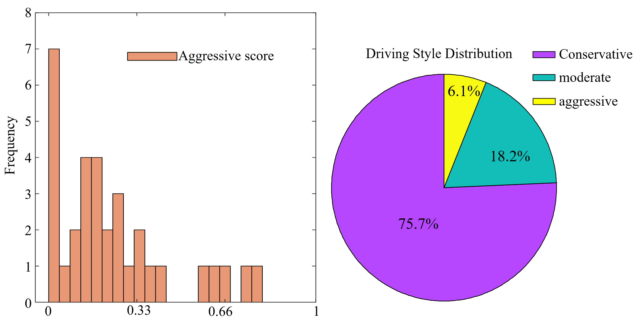
Equation (23) gives the reported aggressiveness-score intervals: conservative for 0 < s < 0.33, moderate for 0.33 < s < 0.66, and aggressive for 0.66 < s < 1.

$$s=\left\{\begin{array}{ll}0<s<0.33,\hfill & \mathrm{Conservative} \mathrm{type}\hfill \\ 0.33<s<0.66,\hfill & \mathrm{Standard} \mathrm{type}\hfill \\ 0.66<s<1,\hfill & \mathrm{Radical} \mathrm{type}\hfill \end{array}\right.$$

(23)

For the subsequent controller, Equation (24) defines one ordinal style code d:

$$d=\left\{\begin{array}{ll}0,\hfill & \mathrm{Conservative} \mathrm{type}\hfill \\ 0.5,\hfill & \mathrm{Standard} \mathrm{type}\hfill \\ 1,\hfill & \mathrm{Radical} \mathrm{type}\hfill \end{array}\right.$$

(24)

In Equation (24), the values 0, 0.5 and 1 respectively represent conservative, moderate and aggressive driving styles. After classifying and marking the driving categories, these values are assigned as equal-interval ordinal codes, indicating the order of each category within the normalized input range.

Thirty-three valid segments were extracted from the available driving data for cluster analysis; the ordered classification results are shown in Figure 6.

2.4.4. Building the Personalized State Vector

The style code obtained in Section 2.4.3 is fused with the vehicle’s real-time states to form the personalized state vector used by the DRL controller.

The state vector is defined as:

$$s_{\mathrm{state}}={\left[v,a,\mathrm{SOC},\alpha ,d,T_{\mathit{req}}\right]}^T$$

(25)

In the equation, a represents the instantaneous acceleration, in m/s².

The six-dimensional state vector combines vehicle speed, acceleration, SOC, road gradient, driving-style code, and demanded torque. The style code allows the Actor to condition its motor-torque and CVT-ratio decisions based on the driving-style category.

2.5. Self-Learning Energy-Management Strategy Based on DDPG

2.5.1. Definitions of State Space and Action Space

The energy-management problem is modeled as a Markov decision process and solved using DDPG. DDPG is selected because the Actor generates continuous motor-torque and CVT-ratio commands without discretizing the action space [31].

The input state space in Equation (25) contains six normalized components: vehicle speed, acceleration, battery SOC, road gradient, ordinal driving-style code, and demanded torque. All continuous state variables are normalized before input, scaling them to the interval [0, 1].

The two-dimensional continuous action in Equation (26) consists of the target motor torque T_m and the CVT transmission ratio i_cvt.

$$a_t={\left[T_m,i_{\mathrm{cvt}}\right]}^T$$

(26)

This operating range directly determines the power distribution between the engine and the electric motor, as well as the operating point of the powertrain.

2.5.2. Reward Function Design

Set a reward function r to guide the agent in reducing fuel consumption while avoiding excessive battery depletion. In the reward function, a negative instantaneous fuel consumption during the control period is added, and a penalty term is added when the SOC is lower than 0.3. The specific formula is as follows:

$$r=-{\dot{m}}_f\cdot \Delta t-\lambda \cdot 1_{\{\mathit{SOC}<{\mathit{SOC}}_{\min }\}}$$

(27)

In Equation (27), Δt represents the control period; λ represents the penalty coefficient for low SOC; and the indicator function takes the value 1 when SOC falls below 0.3 and 0 otherwise.

The first part of this reward function, r_fuel, is the fuel-saving reward term. The negative product of the instantaneous fuel consumption rate and the control period serves as the base reward; that is, the reward at each decision time is negatively correlated with the fuel consumption at that time. Through this design, the lower the fuel consumption, the higher the corresponding reward, thereby guiding the agent to learn energy allocation strategies with better fuel economy.

The second part is r_SOC, the battery constraint penalty. It discourages the controller from over-relying on battery output when minimizing fuel consumption.

2.5.3. DDPG Architecture and Updating

DDPG employs the Actor-Critic framework, in which the Actor outputs deterministic continuous actions and the Critic evaluates their long-term value [17,31,32]. The Critic loss is:

$$L({\theta }^Q)={\displaystyle \frac{1}{N}}{\displaystyle \sum _i{\left(y_i-Q(s_i,a_i|{\theta }^Q)\right)}^2}$$

(28)

In the equation, N represents the number of samples in a small batch; y_i represents the target value computed by the target network; Q(s_i,a_i|θ^Q) represents the Q-value estimate for the state-action pair (s_i,a_i) calculated by the Critic online network; and θ^Q represents the parameters of the Critic online network.

The Target Value y_i is calculated by the target network:

$$y_i=r_i+\gamma Q^{\prime }(s_{i+1},{\mu }^{\prime }(s_{i+1}|{\theta }^{\mu })|{\theta }^{Q^{\prime }})$$

(29)

In Equation (29), r_t represents the reward at the current time step, and γ represents the discount factor. The target Critic evaluates the next state using the action generated by the target Actor. The parameters θ^μ′ and θ^Q′ belong to the target Actor and target Critic, respectively.

In the Actor network, the policy gradient is computed using the chain rule: the gradient of the Critic’s Q-value with respect to the action is multiplied by the gradient of the Actor’s output with respect to its parameters [31]:

$${\nabla }_{{\theta }^{\mu }}J={\displaystyle \frac{1}{N}}{\displaystyle \sum _i{\left.{\nabla }_{a}Q(s,a|{\theta }^Q)\right|}_{s=s_i,a=\mu (s_i)}}{\left.{\nabla }_{{\theta }^{\mu }}\mu (s|{\theta }^{\mu })\right|}_{s=s_i}$$

(30)

In Equation (30), ${\nabla }_{{\theta }^{\mu }}J$ denotes the objective gradient with respect to the Actor parameters. The term ∇_aQ is the gradient of the Critic’s Q-value with respect to the action, and ${\nabla }_{{\theta }^{\mu }}\mu$ is the gradient of the Actor’s output with respect to its parameters. Here, θ^Q denotes the Critic parameters. Averaging the product over the minibatch gives the Actor update direction toward actions with larger estimated Q-values; it does not establish global optimality.

The target network uses soft updating:

$$\left\{\begin{array}{l}{\theta }^{Q^{\prime }}\leftarrow \tau {\theta }^Q+(1-\tau ){\theta }^{Q^{\prime }}\\ {\theta }^{{\mu }^{\prime }}\leftarrow \tau {\theta }^{\mu }+(1-\tau ){\theta }^{{\mu }^{\prime }}\end{array}\right.$$

(31)

In Equation (31), τ is the soft-update coefficient; θ^Q′ and θ^μ′ are the target Critic and target Actor parameters, respectively; and θ^Q and θ^μ are the corresponding online-network parameters. A small soft-update coefficient makes the target networks track the online networks gradually, reducing abrupt changes in the learning targets.

2.5.4. Control Strategy Process

Figure 7 illustrates the overall workflow of the proposed control strategy based on DDPG. In the environment, the state parameters obtained from the operating conditions are used to construct a Gaussian mixture model using the Expectation-Maximization estimation method to obtain a personalized driving model. Plug-in hybrid electric vehicles provide the working parameters and the ordinal style codes of the personalized driving model to form a six-dimensional DDPG state variable input. At each time step, the current state is input into the online actor network, generating control actions including motor torque and CVT transmission ratio; during the training process, exploration noise will be added to enhance the exploration ability of the action space. The generated actions are then applied to the plug-in hybrid electric vehicle model, and rewards and the next state are returned based on the vehicle response. Each state transition is stored in the experience replay buffer. After collecting sufficient samples, the system will randomly select a small batch of data for updating the online actor network and the critic network. At the same time, the target actor and critic networks are updated regularly through a soft update mechanism to improve the stability of the training process.

The DDPG controller was implemented with a six-dimensional state space and a two-dimensional continuous action space. Both Actor and Critic networks consisted of two fully connected layers with 32 ReLU neurons. The Actor generated motor torque and CVT ratio through a tanh output layer, while the Critic estimated the Q-value of state-action pairs. The learning rates of the Actor and the Critic were set to 1 × 10⁻⁴ and 1 × 10⁻³, respectively. A discount factor of 0.99 and a soft update coefficient of 0.005 were adopted. The replay buffer size was 10,000, and the batch size was 32.

Table 3. Controller Architecture and Driving-Style Dataset.

Parameter	Setting
Simulation sampling	0.1 s
State dimension	6
Action dimension	2
Actor network	FC (6-32-32-2), ReLU + tanh
Critic network	FC (8-32-32-1), ReLU + linear
Actor learning rate	1 × 10−4
Critic learning rate	1 × 10−3
Discount factor γ	0.99
Soft update coefficient τ	0.005
Replay buffer size	10,000
Batch size	32
Training episodes	150
Initial exploration noise	0.2
Noise decay	0.995
Minimum noise	0.05
Target network	Soft update as defined in Equation (31)
SOC penalty	Penalty activated below SOC = 0.3
Driving-style dataset	33 valid 60’s CAN-derived segments

summarizes the controller architecture and the dataset used for driving-style analysis.

Because the driving-style code is embedded in the state vector, the Actor can condition its motor-torque and CVT-ratio actions on the identified category.

3. Results

A rule-based control strategy is used as the comparison strategy. This section introduces the simulation platform, evaluates the two strategies under complex driving conditions extracted from CAN data, and analyzes the resulting operating points, SOC, fuel consumption, and control actions.

3.1. Simulation Platform and Boundary Conditions

The MATLAB subsystem model developed in Section 2 constitutes the PHEV simulation model. The DDPG control strategy takes six-dimensional parameters as the input for the state variables and outputs the motor torque and CVT transmission ratio. The rule-based control strategy set is compared with the DDPG control strategy integrated with driving style. Both control strategies are evaluated based on the vehicle model described in this paper and the driving data obtained from the CAN. The vehicle speed is included in the driving data and the controller state, and the road slope is included in the longitudinal dynamics model of the plug-in hybrid electric vehicle.

3.2. Simulation Results

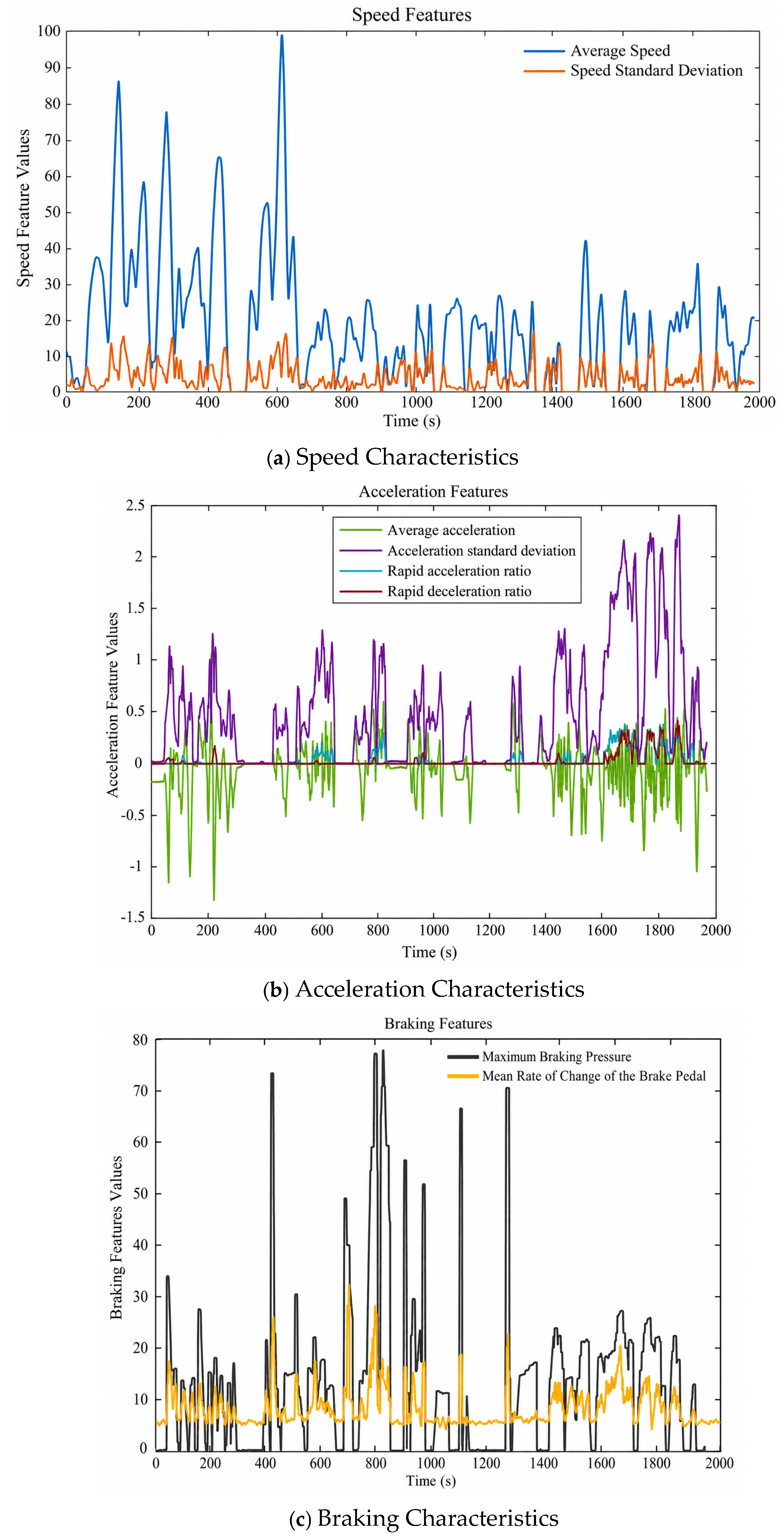
Based on CAN data, complex operating conditions were selected; the operating condition information is shown in Figure 8, including speed characteristics (Average speed $\overline{v}$, standard deviation of speed σ_v), acceleration characteristics (average acceleration $\overline{a}$, standard deviation of acceleration σ_a, proportion of rapid acceleration P_acc, proportion of rapid deceleration P_dec), and braking characteristics (maximum brake pressure P_b,max, mean rate of change of brake pedal pressure $\overline{\left|\dot{p}\right|}$).

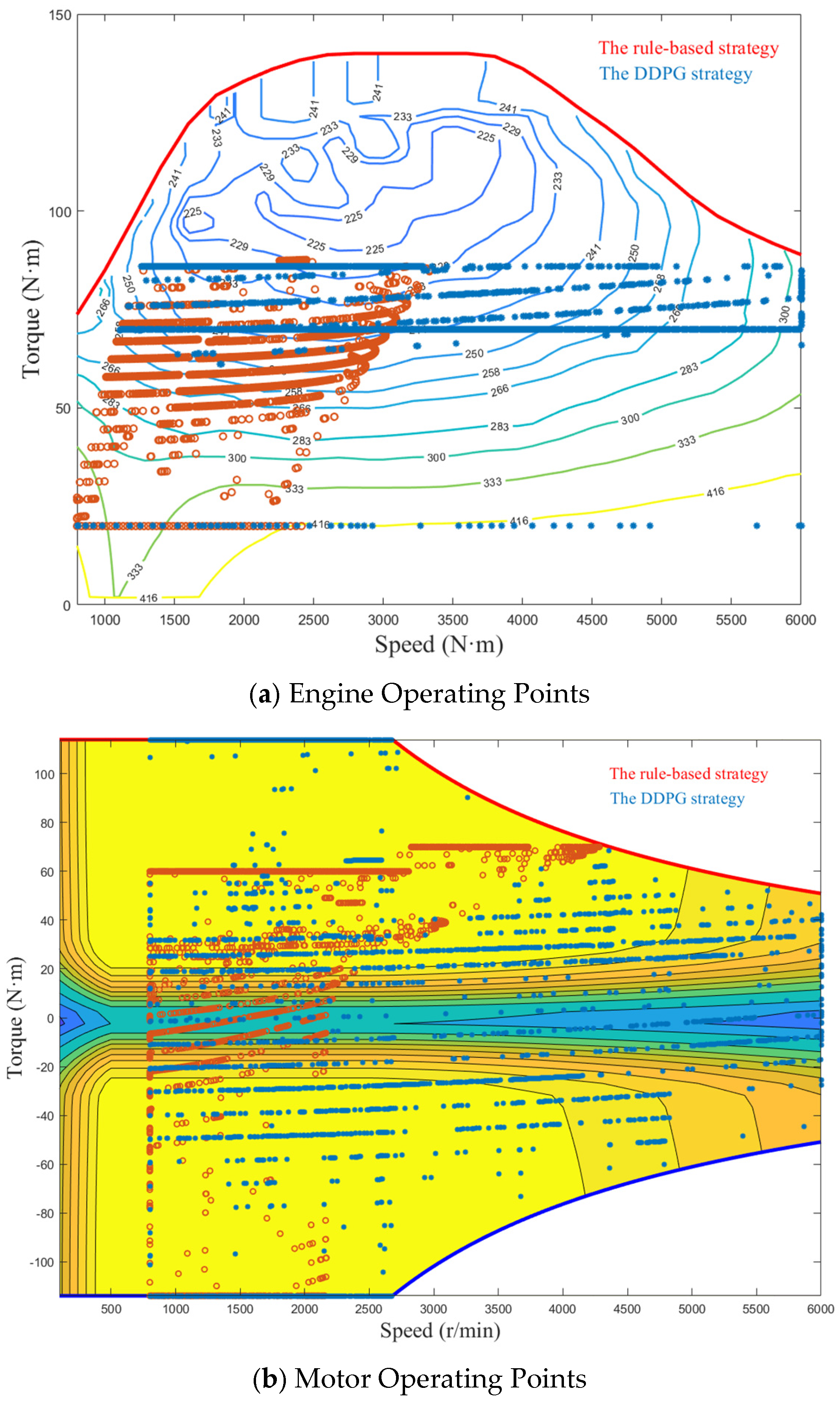
Simulation tests were conducted under the above composite operating conditions for the 1980’s with a sampling interval of 0.1 s. The engine and motor operating points for the two control methods are shown in Figure 9.

As shown in Figure 9a, the engine operating points under DDPG are concentrated near the low-fuel-consumption region of 225–250 g/(kW·h), whereas those under the rule-based strategy are more widely distributed. Figure 9b likewise shows fewer low-efficiency motor operating points under DDPG. These plots provide qualitative operating-point evidence for the integrated controller under the evaluated trajectory.

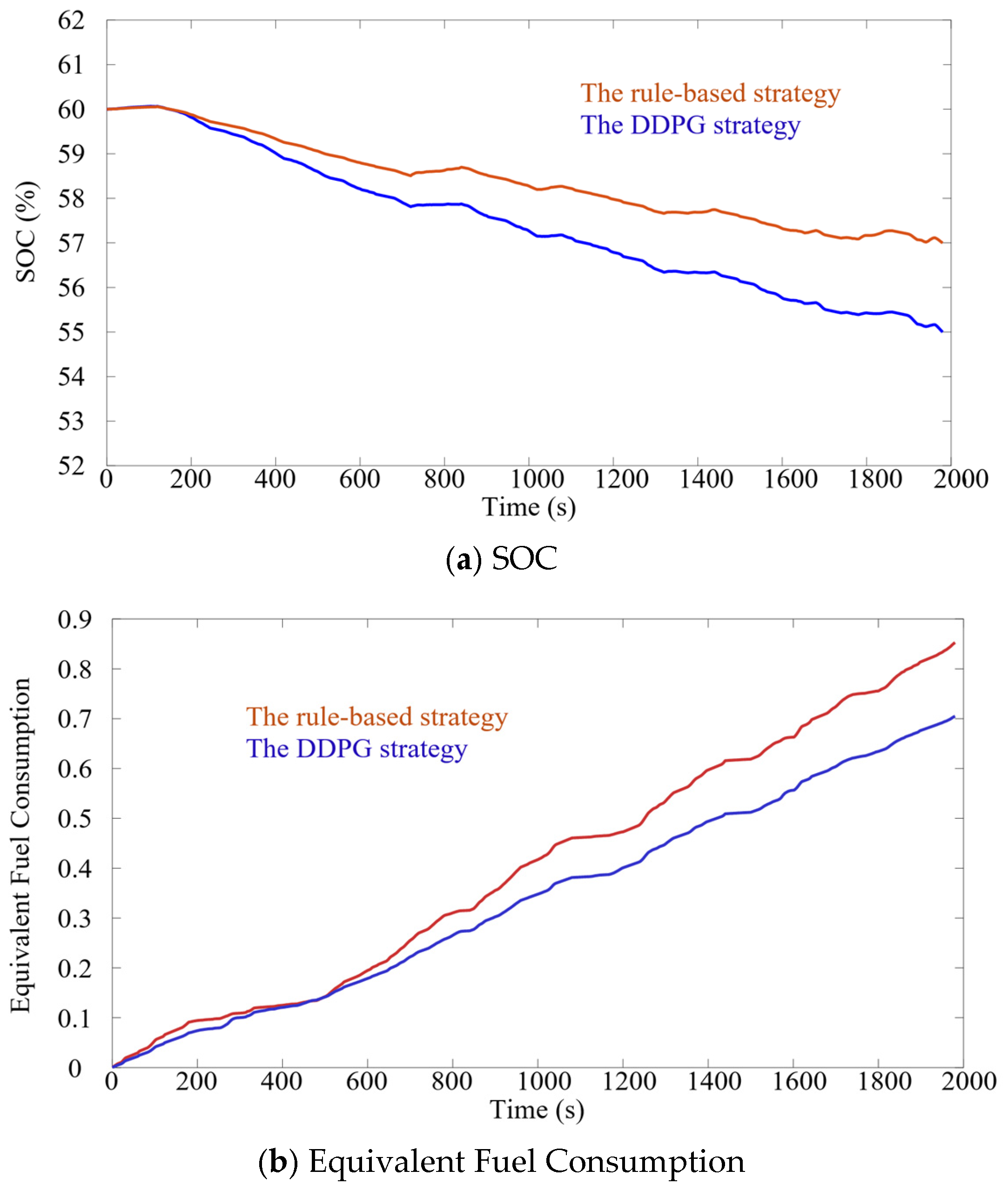
The SOC and equivalent fuel consumption of the two control methods are shown in Figure 10.

As shown in Figure 10, over the 1980’s simulation, the rule-based strategy has an equivalent fuel consumption of 0.853 L, compared with 0.705 L for DDPG. The reported reduction in equivalent fuel consumption is 17.34%. The reported SOC decreases are 2.996% and 4.994%, respectively, indicating greater battery depletion under DDPG.

3.3. Driving-Style Representation and Control Actions

Figure 6 shows the classification of 33 CAN-data segments into three ordered driving-style categories, and Equation (25) includes the category code in the controller state. Figure 9, Figure 10 and Figure 11 and

Table 4. Comparison of Rule-Based and DDPG Results.

Metric	Rule-Based	DDPG	DDPG vs. Rule-Based
Equivalent fuel consumption (L)	0.853	0.705	−17.34%
SOC decrease (%)	2.996	4.994	+1.998
Engine operating region	More dispersed	Concentrated mainly in the 225–250 g/(kW·h) region	Qualitative improvement
Motor operating region	More low-efficiency points	More high-efficiency concentration	Qualitative improvement

present results for the integrated controller.

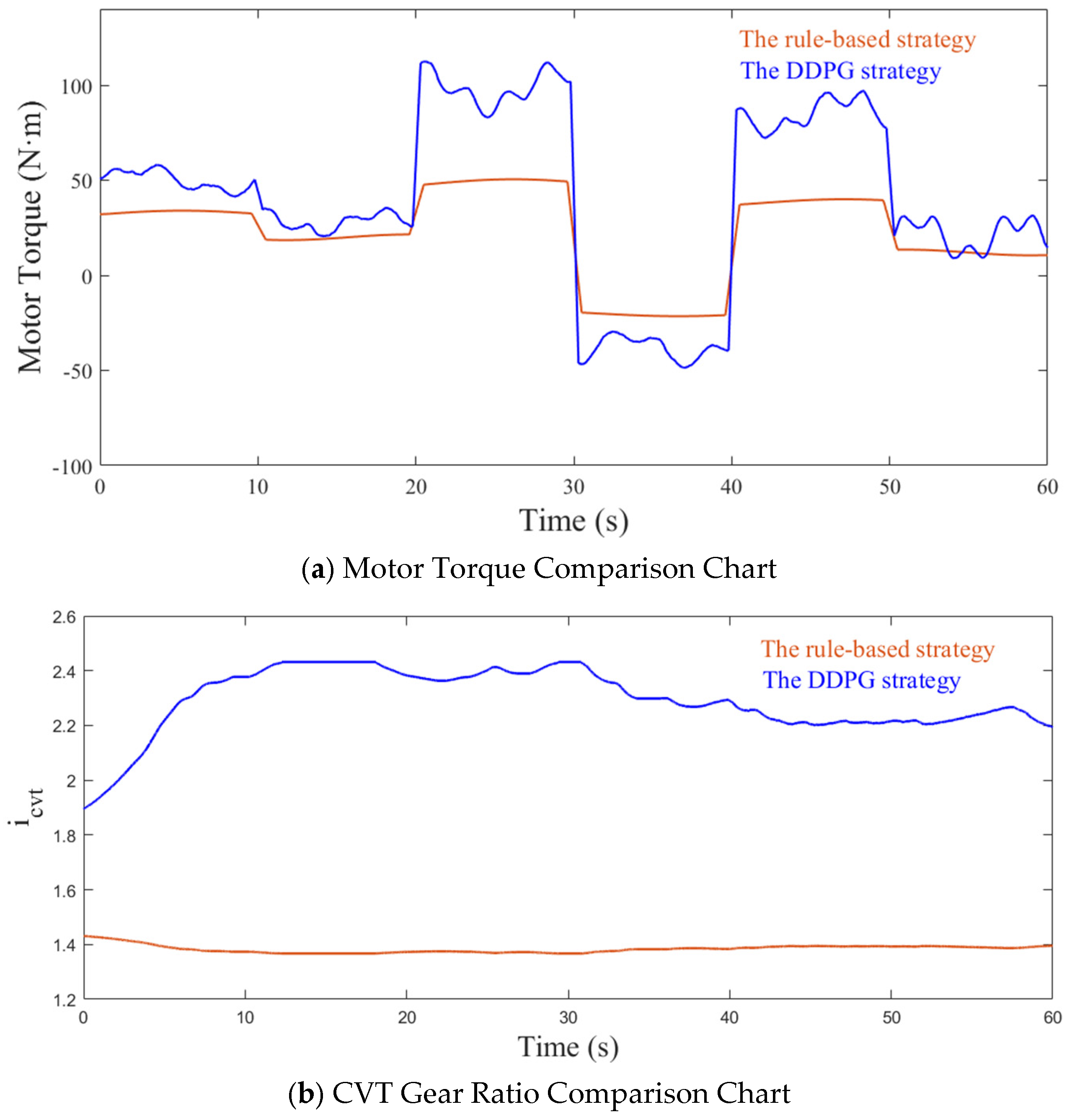
To examine the control actions underlying the aggregate result, a representative 60’s segment is selected. Figure 11 compares motor torque and CVT ratio for the two strategies.

As shown in Figure 11a, DDPG adjusts motor torque more dynamically than the rule-based strategy in the representative 60’s segment. When demanded torque increases, additional motor assistance can shift the engine toward a more efficient operating region. This plot illustrates torque-allocation behavior; the fuel-consumption reduction reported in Table 4 refers to the full 1980’ trajectory, not this segment alone.

As shown in Figure 11b, DDPG adjusts the CVT ratio more frequently than the rule-based strategy in the representative segment. The DDPG strategy can adjust the transmission ratio more flexibly based on the vehicle’s operating conditions. Under complex operating conditions, the DDPG strategy achieves a coordinated match between engine speed and load requirements by promptly adjusting the CVT gear ratio, thereby keeping the engine operating point within the high-efficiency range as much as possible and reducing energy consumption.

In summary, the proposed DDPG personalized energy-management strategy reduces the reported equivalent fuel consumption by 17.34% compared with the rule-based strategy under the evaluated driving trajectory.

4. Discussion

4.1. Comparison with Related Energy-Management Strategies

The results show that combining the CAN-based driving style representation with the DDPG-based energy management controller is feasible. In the evaluated 1980’s composite trajectory, the proposed strategy reduced the equivalent fuel consumption from 0.853 L to 0.705 L, a decrease of 17.34%, compared to the rule-based strategy. The distribution of engine and motor operating points indicates that the DDPG controller operates the power system more frequently in relatively efficient regions. These observations provide a reasonable control-level explanation for the overall fuel consumption results. However, the DDPG strategy also resulted in a higher battery SOC depletion level than the rule-based strategy, and the current comparison was unable to independently distinguish the impact of driving style input on fuel consumption.

Related research has explored the complementary aspects of learning-based energy management. The TD3 method mainly focuses on continuous control, learning stability, and driving condition identification [18,21], while the PPO method is applied to energy management problems involving battery thermal characteristics [19]. Transfer reinforcement learning has been studied for improving the portability of strategies between different vehicle platforms [20], and methods based on SAC have been developed to improve learning efficiency in complex driving cycles and coordinate operation mode decisions [22,33]. Additionally, driving style recognition has been combined with MPC and adaptive ECMS, and evaluated through simulation and hardware-in-the-loop tests [24]. In contrast, this study focuses on introducing the sequential expression of driving style codes extracted from CAN data into the state of the DDPG controller to jointly determine motor torque and CVT transmission ratio. Due to the differences in vehicle configuration, driving cycles, state and action definitions, reward function design, SOC constraint conditions, and verification schemes among these studies, it is necessary to evaluate all algorithms using the same vehicle model, consistent training budget, initial and terminal SOC states, driving cycles, and random seed settings to achieve reliable quantitative comparisons.

4.2. Limitations and Future Work

This research has several limitations. Firstly, the controller only used a single 1980‘s CAN-derived composite trajectory for evaluation, and only compared it with rule-based strategies, without analyzing the standard driving cycle. Secondly, this study did not set up a DDPG strategy that does not rely on driving style input as a control experiment, and thus cannot independently distinguish the effect of driving style from the DDPG controller. Thirdly, it did not match or compare with TD3, SAC, PPO, or other learning-based algorithms. Additionally, due to the need to verify the impact of driving style on the control strategy, multiple random seeds were not used to repeat the runs, thus failing to evaluate its convergence stability and statistical significance. Therefore, the current results have verified the feasibility of the method based on the driving data and evaluation conditions described in the article.

Future research will further enhance the reproducibility of the study. Detailed records of the specific trial procedures and environments will be provided to support independent reproducibility. Future evaluations will include multiple standard driving cycles, hardware-in-the-loop verification, ablation experiments with different driving style inputs, and comparison experiments with other deep learning algorithms. In addition, the driving environment and vehicle auxiliary loads (air conditioning and other auxiliary power demands) will also be taken into consideration and included as further research areas.

5. Conclusions

This paper focuses on plug-in hybrid electric vehicles and addresses the influence of driving-style differences on energy management. It proposes a personalized, self-learning energy-management strategy that integrates multi-feature driving-style analysis with DDPG. The main conclusions are as follows:

(1) The proposed strategy integrates a CAN-derived driving-style representation with DDPG to jointly control motor torque and CVT ratio. MATLAB simulations against a rule-based benchmark demonstrate its feasibility under the evaluated operating conditions.

(2) Under the 1980’s composite trajectory, reported equivalent fuel consumption decreases from 0.853 L for the rule-based strategy to 0.705 L for DDPG, a reported reduction of 17.34%. The reported SOC decreases are 2.996% and 4.994%, respectively. The observed fuel-consumption benefit is accompanied by greater battery depletion.

Further independent-cycle, algorithm-comparison, and experimental validation is planned as described in Section 4.2.

References

1. Wang, Q.; You, S.; Li, L.; Yang, C. Survey on Energy Management Strategy for Plug-in Hybrid Electric Vehicles. J. Mech. Eng. 2017, 53, 1–19. [Google Scholar] [CrossRef] [Scilit]
2. Saiteja, P.; Ashok, B. Critical review on structural architecture, energy control strategies and development process towards optimal energy management in hybrid vehicles. Renew. Sustain. Energy Rev. 2022, 157, 112038. [Google Scholar] [CrossRef] [Scilit]
3. Dong, P.; Zhao, J.; Liu, X.; Wu, J.; Xu, X.; Liu, Y.; Wang, S.; Guo, W. Practical application of energy management strategy for hybrid electric vehicles based on intelligent and connected technologies: Development stages, challenges, and future trends. Renew. Sustain. Energy Rev. 2022, 170, 112947. [Google Scholar] [CrossRef] [Scilit]
4. He, Y.; Hu, Y.; Li, J.; Sun, K.; Yin, J. Multi-scenario driving style research based on driving behavior pattern extraction. Accid. Anal. Prev. 2025, 214, 107963. [Google Scholar] [CrossRef] [Scilit] [PubMed]
5. Yang, N.; Ruan, S.; Han, L.; Liu, H.; Guo, L.; Xiang, C. Reinforcement learning-based real-time intelligent energy management for hybrid electric vehicles in a model predictive control framework. Energy 2023, 272, 126971. [Google Scholar] [CrossRef] [Scilit]
6. Zhao, X.; Wang, L.; Zhou, Y.; Pan, B.; Wang, R.; Wang, L.; Yan, X. Energy management strategies for fuel cell hybrid electric vehicles: Classification, comparison, and outlook. Energy Convers. Manag. 2022, 270, 116179. [Google Scholar] [CrossRef] [Scilit]
7. Li, S.G.; Sharkh, S.M.; Walsh, F.C.; Zhang, C.N. Energy and battery management of a plug-in series hybrid electric vehicle using fuzzy logic. IEEE Trans. Veh. Technol. 2011, 60, 3571–3585. [Google Scholar] [CrossRef] [Scilit]
8. Deng, J.; Wang, Y.; Wang, Y.; Guan, Q.; Liu, Y. Rule-based energy management strategy for hybrid electric vehicles. J. North Univ. China (Nat. Sci. Ed.) 2025, 46, 326–332. [Google Scholar] [CrossRef] [Scilit]
9. Li, S.; Zhao, A.P.; Gu, C.; Bu, S.; Chung, E.; Tian, Z.; Li, J.; Cheng, S. Interpretable deep reinforcement learning with imitative expert experience for smart charging of electric vehicles. IEEE Trans. Power Syst. 2025, 40, 1228–1240. [Google Scholar] [CrossRef] [Scilit]
10. Ren, C.; Liu, H. Optimal energy management strategy of plug-in parallel hybrid electric vehicle based on dynamic programming algorithm. J. Hefei Univ. Technol. (Nat. Sci.) 2021, 44, 1157–1164. [Google Scholar] [CrossRef]
11. Zhang, X.; Yang, L.; Sun, X.; Jin, Z.; Xue, M. ECMS-MPC energy management strategy for plug-in hybrid electric buses considering motor temperature rise effect. IEEE Trans. Transp. Electrif. 2023, 9, 210–221. [Google Scholar] [CrossRef] [Scilit]
12. Liu, J.; Feng, G.; Zhang, J.; Yang, K. Fusion Research of Trajectory Tracking Energy-Saving Control of Unmanned Hybrid Vehicles. China Mech. Eng. 2024, 35, 678–690. [Google Scholar] [CrossRef]
13. He, H.; Wang, Y.; Li, J.; Huang, R.; Chen, J.; Hu, M. Review of machine learning in hybrid electric vehicle energy management. China J. Highw. Transp. 2026, 39, 302–322. [Google Scholar] [CrossRef]
14. Liu, H.; Ma, X.; Han, L.; Xiang, C. Real-time Energy Management Strategy for Hybrid Electric Vehicles Based on Deep Reinforcement Learning and Model Predictive Control. J. Mech. Eng. 2026, 62, 302–313. [Google Scholar] [CrossRef] [Scilit]
15. Shao, J.-K.; Hu, M.-H.; Ma, Z.-A.; Zhang, S.-J.; Li, Z.-H. Predictive Energy Management Strategy for Plug-in Hybrid Electric Vehicles Based on Driving Condition Recognition. J. Jilin Univ. (Eng. Technol. Ed.) 2026, 1–15. [Google Scholar] [CrossRef]
16. He, H.; Meng, X.; Wang, Y.; Khajepour, A.; An, X.; Wang, R.; Sun, F. Deep reinforcement learning based energy management strategies for electrified vehicles: Recent advances and perspectives. Renew. Sustain. Energy Rev. 2024, 192, 114248. [Google Scholar] [CrossRef] [Scilit]
17. Zhuang, J.; Li, P.; Liu, L.; Ma, H.; Cheng, X. Energy Management Strategy for Hybrid Electric Vehicles Based on Experience-Pool-Optimized Deep Reinforcement Learning. Appl. Sci. 2025, 15, 9302. [Google Scholar] [CrossRef] [Scilit]
18. Wu, C.; Ruan, J.; Cui, H.; Zhang, B.; Li, T.; Zhang, K. The application of machine learning-based energy management strategy in a multi-mode plug-in hybrid electric vehicle, Part I: Twin delayed deep deterministic policy gradient algorithm design for hybrid mode. Energy 2023, 262, 125084. [Google Scholar] [CrossRef] [Scilit]
19. Zhang, C.; Li, T.; Cui, W.; Cui, N. Proximal policy optimization based intelligent energy management for plug-in hybrid electric bus considering battery thermal characteristic. World Electr. Veh. J. 2023, 14, 47. [Google Scholar] [CrossRef] [Scilit]
20. Huang, R.; He, H.; Su, Q.; Härtl, M.; Jaensch, M. Enabling cross-type full-knowledge transferable energy management for hybrid electric vehicles via deep transfer reinforcement learning. Energy 2024, 305, 132394. [Google Scholar] [CrossRef] [Scilit]
21. Guo, J.; Wang, Y.; Chen, J.; Li, H.; Gui, A. Energy management strategy for plug-in hybrid electric vehicles based on twin delayed deep deterministic policy gradient algorithm and condition recognition. Energy Technol. 2025, 13, 2500482. [Google Scholar] [CrossRef] [Scilit]
22. Huang, R.; He, H.; Su, Q. Smart energy management for hybrid electric bus via improved soft actor-critic algorithm in a heuristic learning framework. Energy 2024, 309, 133091. [Google Scholar] [CrossRef] [Scilit]
23. Zhu, P.; Hu, J.; Li, J.; Peng, H.; Wang, X. Co-optimization Method for Personalized Eco-adaptive Cruise Control of Plug-in Hybrid Electric Vehicles Considering Uncertainties in Driving Style. J. Mech. Eng. 2025, 61, 214–229. [Google Scholar] [CrossRef] [Scilit]
24. Wang, R.; Yang, Y.; Sun, X.; Wen, Y.; Cao, Y. Model predictive control for PHEBs based on driving style recognition in car-following scenarios. Adv. Mech. Eng. 2026, 18, 16878132261442709. [Google Scholar] [CrossRef] [Scilit]
25. Gao, X. Research status and development trend analysis of hybrid electric vehicle control strategies. Spec. Purp. Veh. 2022, 10, 22–24. [Google Scholar] [CrossRef]
26. Xu, L.; Tao, Y.; Zhang, J.; Wen, C.; Wang, D.; Liu, M.; Yan, X. Hierarchical Cooperative Control Strategy of Unmanned HMCVT Tractor Considering Trajectory Tracking Performance and Economy. Trans. Chin. Soc. Agric. Mach. 2025, 56, 61–72+123. [Google Scholar] [CrossRef]
27. Zhang, J.; Feng, G.; Yan, X.; He, Y.; Liu, M.; Xu, L. Cooperative control method considering efficiency and tracking performance for unmanned hybrid tractor based on rotary tillage prediction. Energy 2024, 288, 129874. [Google Scholar] [CrossRef] [Scilit]
28. Sun, W.; Zhang, D.; Zou, Y.; Zhang, X.; Zhang, J. Intelligent Adaptive Energy Management Strategy for Dual-APU Hybrid Heavy-Duty Vehicles. Automot. Eng. 2026, 48, 1169–1180. [Google Scholar] [CrossRef]
29. Zhang, L.; Wu, G.; Wang, Y. Unified Modeling and Verification of Vehicle Longitudinal/Lateral/Vertical Dynamics. J. Mech. Eng. 2019, 55, 114–122. [Google Scholar] [CrossRef] [Scilit]
30. Song, Z.; Zhang, S.; Li, W.; Gan, Y.; Ding, H. Sensitivity analysis and uncertainty bounding of tire parameters on vehicle handling and stability. Nonlinear Dyn. 2025, 113, 11446. [Google Scholar] [CrossRef] [Scilit]
31. Lillicrap, T.P.; Hunt, J.J.; Pritzel, A.; Heess, N.; Erez, T.; Tassa, Y.; Silver, D.; Wierstra, D. Continuous control with deep reinforcement learning. arXiv 2015, arXiv:1509.02971. [Google Scholar] [CrossRef] [Scilit]
32. Tang, X.; Chen, J.; Pu, H.; Liu, T.; Khajepour, A. Double Deep Reinforcement Learning-Based Energy Management for a Parallel Hybrid Electric Vehicle with Engine Start-Stop Strategy. IEEE Trans. Transp. Electrif. 2022, 8, 1376–1388. [Google Scholar] [CrossRef] [Scilit]
33. Zhou, J.; Zhang, T.; Zhang, H.; Zhang, Z.; Hong, J.; Yang, J. Energy management strategy for electro-hydraulic hybrid electric vehicles considering optimal mode switching: A soft actor-critic approach trained on a multi-modal driving cycle. Energy 2024, 305, 132172. [Google Scholar] [CrossRef] [Scilit]
Figure 1. Overall Framework of CAN-Based Driving-Style Identification and DDPG Energy Management.
Wevj 17 00522 g001
Figure 2. Plug-in Hybrid Electric Vehicle Architecture.
Wevj 17 00522 g002
Figure 3. Engine Performance Map.
Wevj 17 00522 g003
Figure 4. Motor Efficiency Map.
Wevj 17 00522 g004
Figure 5. Schematic Diagram of the Full-Vehicle Simulation Model.
Wevj 17 00522 g005
Figure 6. Distribution of Driving Styles and Clustering Results.
Wevj 17 00522 g006
Figure 7. DDPG Training and Control Workflow.
Wevj 17 00522 g007
Figure 8. CAN-Derived Operating Conditions.
Wevj 17 00522 g008
Figure 9. Engine and Motor Operating-Point Comparison.
Wevj 17 00522 g009
Figure 10. SOC and Equivalent Fuel Consumption for the Two Control Methods.
Wevj 17 00522 g010
Figure 11. Motor-Torque and CVT-Ratio Comparison for a Representative Segment.
Wevj 17 00522 g011