Next Article in Journal
Multi-Objective Lightweight Optimization and Decision for CTB Battery Box Under Multi-Condition Performance
Next Article in Special Issue
LSON-IP: Lightweight Sparse Occupancy Network for Instance Perception
Previous Article in Journal
SBF-DRL: A Multi-Vehicle Safety Enhancement Framework Based on Deep Reinforcement Learning with Integrated Safety Barrier Function
Previous Article in Special Issue
Electric Vehicles and Urban Tourism in Smart Cities: A Bibliometric Review of Sustainable Mobility Trends and Infrastructure Development
error_outline You can access the new MDPI.com website here. Explore and share your feedback with us.
 
 
Article

A Vehicle Routing Optimization Framework of a Property City Based on an Intelligent Algorithm and Its Application

1
Digital Intelligence Management Research Institute, Shanghai University of Finance and Economics Zhejiang College, Jinhua 321015, China
2
School of Economics and Management, Jiaying University, Meizhou 514015, China
3
Wenzhou Sapphires Property Management Co., Ltd., Wenzhou 325099, China
4
Zhejiang Limin Environmental Technology Co., Ltd., Jinhua 310005, China
*
Authors to whom correspondence should be addressed.
World Electr. Veh. J. 2026, 17(1), 25; https://doi.org/10.3390/wevj17010025
Submission received: 22 October 2025 / Revised: 16 December 2025 / Accepted: 26 December 2025 / Published: 6 January 2026

Abstract

Property city is a newly emerging property service mode attracting widespread attention. Addressing the gap in quantitative analysis of the vehicle routing problem (VRP) of a property city based on quantitative analysis in existing studies, this study introduces the single-loop traveling salesman problem (TSP) and multi-loop VRP models for different service scenarios of a property city. An intelligent optimization framework combining the nearest insertion method and genetic algorithm was constructed to solve these problems. The example analysis results show that the intelligent algorithm is feasible, outperforming the nearest insertion method in designing reasonable operational schemes, while the total operational cost of the multi-loop scenario was lower than that of the single-loop scenario. This study enriches the theoretical system of property city and provides references for its service practice.

1. Introduction

Property service mode innovation is the basic problem of the operation of property service enterprises. Vanke Property Development Co., Ltd., in China first proposed the “property city” service mode for its Hengqin project in 2018. The service mode of a property city has a great impact on the property service industry. A property city takes the city as a whole as a “big property” and integrates resources through “professional services + smart platform + administrative force”. Property city mode outsources the urban public service as a whole through a professional service package, modular service division of labor, socialized governance structure, and refined governance means. Property city mode adopts the whole-process “management + service + operation” collaborative governance mode for urban public space, which is essentially the expansion and application of traditional property services in urban public space [1]. Shen et al. [2] took the urban governance project of Hengqin as an example to summarize the new mode of property city management, elaborate the concept, implement the rules and feasibility of property city, and put forward relevant policy suggestions for the implementation of property city. Sun et al. [3] discussed the development status of property cities from the perspective of urban governance and summarized foreign urban governance and its inspiration on property city. As a new mode of property service, the service scenario of property city has undergone great changes, posing a new challenge to its vehicle route optimization.
There are many methods in theory and practice that can be applied to the problems of property service and route optimization. Scholars have successively used SERVQUAL [4], cluster analysis [5], and other methods for property service evaluation. In addition, the methods that can be used to solve such problems are multidimensional preference analysis linear programming (LINMAP) [6], MARCOS [7], EDAS [8], social network [9], consensus decision making [10], and so on. Among them, econometric analysis based on the SERVQUAL model is the most commonly used method in property service quality. Based on the optimization method perspective, Zuo’s research team introduced methods such as the technique for order preference by similarity to ideal solution (TOPSIS), multi-attribute multi-scale (MIMS), LINMAP and interactive multi-attribute decision making (TODIM), solving the property service quality management problem of a large group, multi-stage [11], multi-source heterogeneity [12], and considering the degree of group rationality [5]. On the other hand, the vehicle routing problem (VRP), proposed by Dantzig and Ramser [13], is a hot topic in supply chain research [14]. The VRP is a classic combinatorial optimization problem that involves determining the best path for a set of vehicles to meet the needs of a set of customers while minimizing total cost or total distance [15]. Regarding the VRP, it can be traced back to the traveling salesman problem (TSP) describing a knight travel problem in 1759 [16], also known as the traveling merchant problem. The VRP is an extension of the TSP. Since Gaery proved that the TSP is an NP problem, the VRP is also an NP problem [17]. Intelligent algorithms provide a broad space for solving such problems and thus develop into intelligent optimization algorithms. Intelligent algorithms usually used to solve the VRP mainly include the Bayesian network [18], ant colony algorithm [19], and particle swarm algorithm [20]. Among them, the genetic algorithm is the most common intelligent algorithm for path planning [21].
The TSP model, VRP model, and genetic algorithm have been paid much attention to in academic circles. In the research on TSP models, scholars have carried out in-depth exploration for its computational complexity and practical application requirements. Dong et al. [22] proposed the cooperative genetic ant system to solve the large search space and the existence of a large number of local optimal solutions in the space, while the ant colony algorithm has problems in achieving the global optimal solution of the TSP. Applegate [23] conducted in-depth research on the theoretical properties of the TSP, which provides an important theoretical basis for subsequent algorithm design. Bouhmala [24] proposed a multi-objective genetic algorithm that can simultaneously consider multiple optimization objectives for the TSP, such as path length and number of vehicles. In the research of the VRP model, the focus of the scholars’ research lies in how to find the optimal route under complex constraints. Subsequently, Srivastava and Singh [25] proposed two evolutionary methods with target-specific mutation operators to solve the problem of three target vehicle routing with time window and quality of service objectives, aimed at improving service quality. Tutumlu and Sarac [26] proposed a hybrid genetic algorithm for large problems where the mathematical model cannot find a feasible solution. To solve the optimization problem, Le et al. [27] proposed a new deep learning-based joint optimization algorithm for UAV positioning and power allocation. In the research of genetic algorithms, scholars have not only made remarkable achievements in combinatorial optimization problems such as the TSP and VRP but also applied it to other fields. In addition, Goldberg [28] systematically introduced the theory and application of genetic algorithms in his books and made important contributions to the popularization and promotion of genetic algorithms. Talbi et al. [29] proposed a new algorithm that is superior to the standard genetic algorithm to solve the TSP. By comparing the genetic algorithm in the evolutionary computing field and the Epsilon–Greedy Q-Learning Algorithm (EQLA) in machine learning and the field to solve the TSP, Uthayasuriyan [30] concluded that the genetic algorithm is more effective than the EQLA in solving TSP. There have been some studies related to the VRP based on the genetic algorithm. Yusuf et al. [31] conducted a study on the effectiveness of a genetic algorithm for the VRP. Vaira and Kurasova [32] proposed a genetic algorithm based on the insertion heuristic to solve the VRP with constraints. Wang and Huang [33] proposed a VRP model specifically for emergency situations.
To sum up, the existing evaluation frameworks based on criteria for making trade-offs are unable to effectively address the complex optimization problems in property city service mode. The service mode of property city has attracted much attention, but there is a lack of discussion on quantitative analysis based on intelligent optimization algorithms. Research on the TSP, VRP, and genetic algorithms is relatively abundant, but the existing research cannot provide a complete framework for property city vehicle routing optimization. Therefore, this paper adopted a hybrid strategy combining the genetic algorithm and the nearest insertion method, aiming to efficiently solve the NP-hard problem of vehicle routing for property city. The reason for choosing the genetic algorithm is its powerful global search capability, which can effectively handle multiple constraints and avoid local optima, thereby obtaining a high-quality overall optimization solution. The main reason for introducing the nearest insertion method is to generate a high-quality initial population for the genetic algorithm, significantly accelerating the convergence process. At the same time, the nearest insertion method itself is computationally efficient and is also suitable for handling dynamically added service requests. The insertion method combined with the genetic algorithm can balance the efficiency and quality of the solution, perfectly meeting the dual requirements of real-time performance and economic efficiency in property management and urban management. The main innovation points of this paper are as follows: on the one hand, the research of property city theory and application is enriched by quantitative analysis based on an intelligent algorithm; on the other hand, a vehicle routing optimization framework including an optimization model and intelligent algorithm is constructed.
The follow-up arrangement of this paper is as follows: Section 2 puts forward the overall analysis framework of this study based on single-area and multi-area vehicle transportation; Section 3 describes the basic principles of property city vehicle routing optimization analysis based on the TSP, VRP, and genetic algorithm; Section 4 analyzes an example of property city vehicle routing optimization based on the intelligent optimization algorithm; and Section 5 includes research conclusions, innovation points, and future research prospects.

2. Analysis Framework

Since the operational area of a single property city is usually quite large, this paper divides the operational area of a single property city into two types: single-region vehicle transportation and multi-region vehicle transportation. The former is a single-loop TSP problem, while the latter is a multi-loop VRP problem. Based on the solution of the two transportation problems, the intelligent optimization algorithm is used, and the results are analyzed to seek the optimal solution of planning of the project. The analysis results are used to assist in the design of solutions for property city vehicle routing.

2.1. Single-Area and Multi-Area Transportation

(1) Single-area transportation scenario. In single-area transportation scenario, route mileage, labor cost, and water load are considered, and the nearest insertion method and genetic algorithm are used to solve the shortest path of entire operating area under the goal of minimum cost. The single-area transportation scenario is set to adopt the solution of the path optimization under a single vehicle. In this scenario, a single vehicle is used to operate in the entire operating area, and the single vehicle traverses all points to achieve the shortest driving distance. The single-area transportation problem has an obvious single character and ergodic character. At this time, the operating vehicle can achieve full coverage within the entire operating area, and the content considered is more comprehensive. However, the goal of a single-loop TSP is relatively simple, focusing more on the solution of the shortest realization path, as well as considering less factors such as time cost and efficiency cost.
(2) Multi-area transportation scenario. The factors considered in the multi-area transportation scenario are the same as those in the single-area transportation scenario. The entire operating area is divided by the scanning algorithm, and each subarea can be regarded as a TSP. It is required to solve the shortest path of the entire operating area to achieve the goal of minimizing the total cost. The multi-area transportation scenario is set to adopt an area path solution under multi-vehicles, considering the entire operating area, vehicle load limit, vehicle mileage limit, and other factors. In the multi-area transportation scenario, multiple vehicles are used to operate in the entire operating area, and the interference factors are eliminated and weakened. The goal is to achieve the multi-loop transportation of multiple vehicles in the entire operating area with minimum cost. At this time, the time cost of route running, manual operation, and efficiency cost of route planning are also taken into account, and the advantages of multiple vehicles operating together can be used to achieve the optimization of multiple objectives. However, the solution of multi-loop VRP is complicated, which puts forward higher requirements for process management.

2.2. Overall Analysis Framework Design

Based on the above analysis, the single-loop TSP and multi-loop VRP are, respectively, used to solve the vehicle routing optimization problem of a property city. For the single-loop TSP, the results of nearest insertion method and genetic algorithm are compared and analyzed, and the optimal solution of single-area vehicle routing is obtained. For the multi-loop VRP, the optimal solution of the multi-area path is obtained by comparing the results of the nearest insertion method and genetic algorithm. Finally, by comparing the solutions of the two models mentioned above, the final solution to the aforementioned problem is obtained. The research framework of this paper is shown in Figure 1.

3. Basic Principles

3.1. TSP Model and Nearest Insertion Method

(1) The TSP model. The TSP model setup: A traveling salesman starts from a certain city, sells goods in n cities, visits each city once and only once, and then returns to the original city. The TSP model is suitable for the single-area transportation scenario. The problem lies in determining which route the traveling salesman should take in order to minimize the total travel distance (or the least travel cost). Usually, the TSP is a typical NP-Hard problem. The TSP model can be described as follows: given a connected graph with n directed or undirected vertices, a loop containing n vertices with the smallest total weight (distance, cost, time, etc.) is sought. The mathematical description of the TSP model is as follows:
m i n z = i = 1 n j = 1 n c i j x i j
s t :   j = 1 n c i j = 1 , i = 1,2 , , n
i = 1 n x i j = 1 , j = 1,2 , , n
i , j : i , j = 2 , , n ; x i j = 1
x i j 0,1 , i = 1,2 , , n ; j = 1,2 , , n
where the decision variable x i j = 0 denotes the edge not connected i to j , x i j = 1 denotes the edge not connected i to j , c i j denotes the weight of the edge connected i to j , Equation (2) denotes that only one edge goes out of each vertex, and Equation (3) denotes that only one edge enters each vertex; moreover, only the two constraints of Equations (2) and (3) may have the subloop phenomenon, that is, there are multiple loops. Therefore, it is necessary to add the constraint of Equation (4), that is, other selected edges do not constitute loops except for the starting edge and the ending edge.
(2) Nearest insertion method. The nearest insertion method was first proposed by Rosenkrantz et al. in 1977 [34]. As an algorithm used to solve the TSP, the nearest insertion method can be completed through four steps:
① Find the point with the smallest distance from c 1 k and form a subloop ( v 1 , v k ) .
② Among the remaining points, find a point that is closest to a point in the subloop.
③ Find an arc ( i , j ) in the subloop, so that c i k + c k j c i j is minimum, and then add the point v k to the subloop, insert the point v i and v j ; and replace the original arc ( i , j ) with two new arcs ( i , k ) and ( k , j ) .
④ Repeat steps ② and ③ until all points are added to the subloop.

3.2. VRP Model and Its Solution

(1) The VRP model. The VRP model setup: For a series of delivery points and receiving points, call certain vehicles and organize appropriate driving routes so that vehicles pass through them in an orderly manner and achieve certain goals under the specified constraints. That is, strive to achieve the shortest total distance of empty vehicles and the lowest total transportation cost, where vehicles arrive at a certain time and other goals. The VRP is common in deployment practices, especially when there are a large number of service objects. When solving this kind of allocation problem, the core is how to schedule the vehicles. The VRP model can be described as follows:
① Basic condition: There are m identical vehicles parked at a common source point v 0 , which need to provide goods to n customers, denoted as v 1 , v 2 ,…, v n .
② Model objective: To determine the number of required vehicles N and assign these vehicles to a loop, including routing and scheduling within the loop, so that the total transportation cost C is minimized.
③ Restriction conditions: a. N m ; b. Every order must be fulfilled; c. Each vehicle must return to the starting point after completing the mission; d. The capacity limit of the vehicle cannot be exceeded, and the limit of the time window need be considered; e. Restrictions on transport regulations.
(2) Solution ideas. There are many classification methods for vehicle route scheduling problems. When using the VRP model to solve practical problems, it is necessary to consider the warehouse, vehicle, time window, customer, road information, cargo information, transportation regulations, and other factors. For different route problems, the models of the vehicle scheduling problem are also very different. In order to simplify the solution of the vehicle scheduling problem, some techniques are often used to decompose or transform the problem into one or several basic problems that have been studied, and then relatively mature methods are used to obtain the optimal or satisfactory solution of the original problem. Therefore, the basic idea of solving the VRP model in this study is as follows: according to certain requirements, the entire operation area is divided into several subareas, each of which can be described by the TSP model. Obviously, compared with solving the TSP model, the key to solving the VRP is the partition method. The commonly used partitioning methods include the mileage saving method, scanning algorithm, and so on. When solving complex problems, the division should also take into account the actual situation.

3.3. Genetic Algorithm

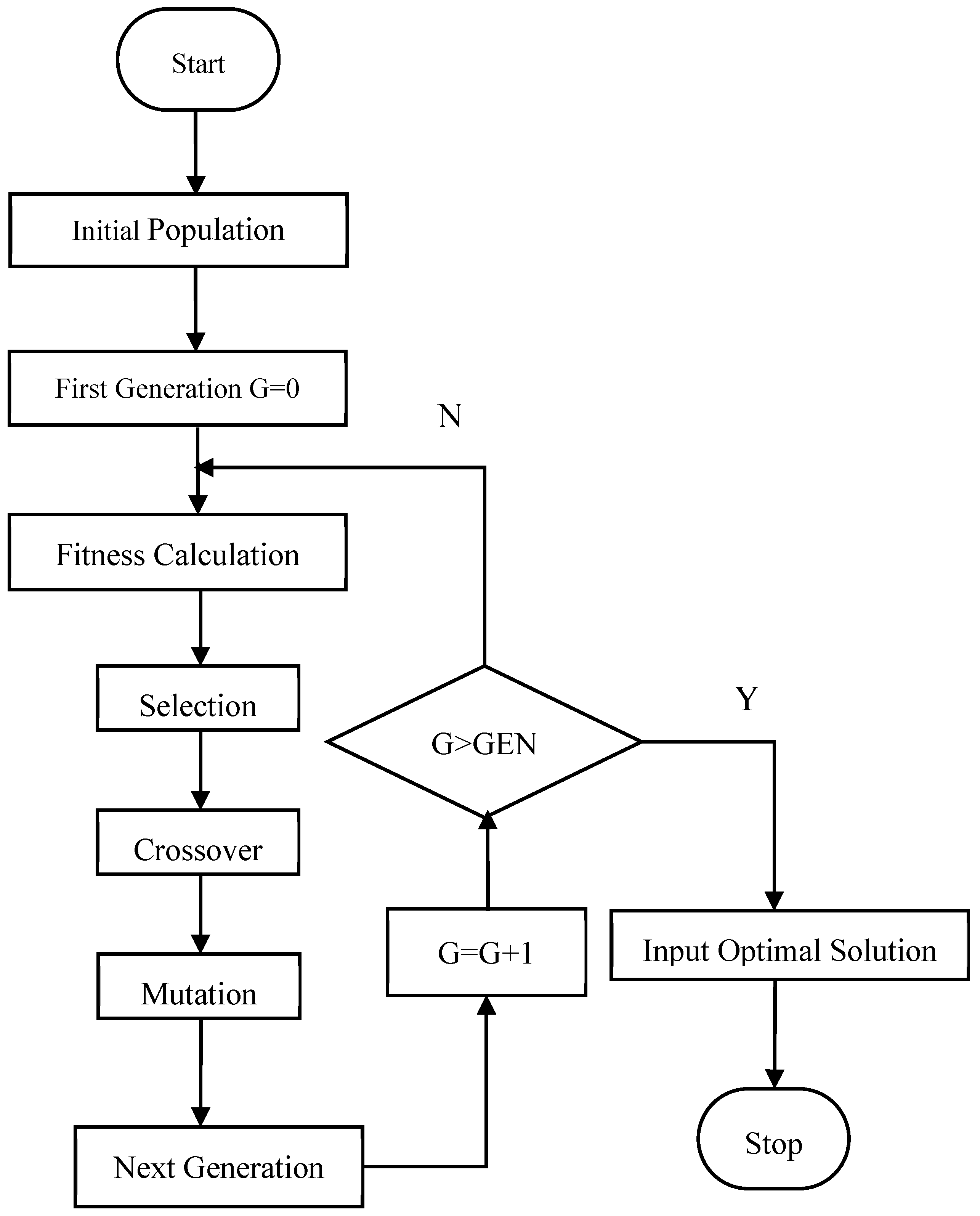
(1) Basic principles. The genetic algorithm is a kind of optimization technology based on natural selection and biological genetic mechanisms, one that draws reference from the biological evolution process. It relies on a natural stochastic algorithm to approximate the optimal solution of the problem, and it has good global search ability. To solve a problem through the genetic algorithm, the parameters of the problem are encoded in a certain form, and the encoded bit string is called a chromosome. Through the genetic operators (selection, crossover, mutation), a group of new chromosomes that are more adaptable to the environment can be generated to form a new population. In this way, generations continue to reproduce, evolve, and finally converge into a group of individuals who are most adaptable to the environment, and the optimal solution to the problem can be obtained. The main links of the genetic algorithm are described as follows:
① Coding. A chromosome or individual representing the genetic space by encoding the problem to be solved.
② Choose. According to individual fitness and certain rules, select excellent individuals to be inherited by the next generation. The roulette selection method is the most commonly used method in the genetic algorithm, being a proportional selection, wherein the probability of each individual being selected is proportional to its fitness function value. If the fitness of an individual i is f i and the population size is NP, then the probability that the individual i is selected is Pi = f i / i = 1 N P f i ( i = 1,2 , , N P ) .
③ Crossover. Crossover is a key operator in genetic algorithms, referring to the process of recombining genetic segments between two parent chromosomes to generate new offspring. It significantly enhances the algorithm’s search capability. As the core operator of basic genetic algorithms, crossover simulates biological genetic recombination. Its principle is to select higher-fitness parent chromosomes, randomly set crossover points, and exchange corresponding gene segments. Functions include inheriting superior genes, generating new gene combinations, maintaining population diversity, avoiding premature convergence, and aiding in approaching the optimal solution. Order crossover steps are as follows: First, select two parent chromosomes. Second, randomly determine two non-overlapping cut points. Third, copy the substring between the cut points from the first parent directly to the corresponding positions in the offspring. Lastly, starting from the position after the second cut point in the second parent, sequentially select genes not present in the offspring’s substring to fill remaining positions; resume from the start of the second parent if its end is reached.
④ Mutation. Multiple mutations include reverse mutation (main) + exchange mutation (auxiliary). The core logic of reverse mutation is to randomly select a continuous sub-path and reverse (reverse-arrange) it. The operation steps are as follows: randomly select two different cutting points (i < j), determine a continuous sub-path (from the i-th position to the j-th position); reverse this sub-path (for example, [a,b,c] → [c,b,a]); the cities at other positions remain unchanged, and a new path is obtained. The core logic of the exchange mutation is to randomly select two different cities from the path and swap their positions. The operation steps are as follows: randomly pick two different index positions (for example, the i-th position and the j-th position, where i ≠ j) from the path; swap the cities at these two positions; and obtain a new path (naturally without repetition or omission). The actual operation steps are as follows: First, use the order crossover as the main crossover operator to preserve the structure of the parent sub-strings. Second, use reverse mutation as the main mutation operator (medium-scale perturbation, equivalent to segment inversion, suitable for TSP problems), and set the initial reverse mutation probability to 0.1 to 0.2. Third, use the exchange mutation as an auxiliary operator, and set the initial exchange mutation probability to 0.01 to 0.05. Fourth, perform crossover first and then mutation. If the computational budget allows, apply lightweight local search to the elite individuals to accelerate convergence. Finally, monitor the population diversity and convergence rate: when stagnation occurs, increase the reverse mutation probability for stronger exploration; when approaching the optimal solution, increase the exchange mutation probability.
⑤ Termination condition. When the fitness of the optimal individual reaches a given threshold, or the fitness of the optimal individual and the fitness of the population no longer rises, or the number of iterations reaches a preset algebra, the algorithm terminates.
(2) Algorithm description. The description of the genetic algorithm is shown in Figure 2.
The genetic algorithm adopted in this paper is described as follows:
① Set evolutionary algebraic counting t = 0 and initialize the population P ( t ) .
② Calculate the fitness value of each individual in the population P ( t ) . If each bit of the gene of an individual in the population is all 0, a smaller fitness value is assigned to the individual.
③ The population P ( t ) is obtained by proportional selection operation on the population P ( t ) .
④ Perform crossover and mutation operations on P ( t ) , and obtain the next generation population P ( t + 1 ) .
⑤ If the change is small within 10 generations or t = t h e   n u m b e r   o f   m a x i m u m   e v o l u t i o n a r y   g e n e r a t i o n s when (set in advance) it ends, otherwise turn ①.
(3) Operating parameters and environment. The descriptions of population size, mutation rate, stopping condition, and operating environment are as follows:
① The population size ranges from 50 to 200, and the main observation is the number of necessary points within the population, that is, the number of coordinate axes identified by the scanning algorithm.
② The range for setting the mutation rate is mainly between 0.001 and 0.05. By traversing the results, an optimal shortest path is obtained. Too high (e.g., Pm > 0.05): The algorithm degenerates into “random search”, losing the optimization advantage of the genetic algorithm. Too low (e.g., Pm < 0.001): It is unable to supplement new genes and is prone to getting stuck in local optimum.
③ By traversing the mutation rate from high to low at a distance of 0.005, an optimal output result (the shortest distance) is obtained as the model result. If the distance is shorter than the original distance, the calculated distance later will be taken as the result, and the original distance will be recorded. It will be plotted in the graph.
④ Operating environment is Pycharm.

4. Example Analysis

Zhejiang Limin Environmental Technology Co., Ltd. in China. (hereinafter referred to as Limin Environment), is a pioneer in property city operation. The Xiaoshun Project of Limin Environment has a long operation time, a wide range of services and high equipment investment, and has a good foundation for property city operation. Therefore, this paper chose the Xiaoshun Project as the research area. Using the basic method proposed above, this paper analyzed the vehicle routing optimization problem of the water and dust removal operation in the Xiaoshun Project, and it produced a comparative analysis of the results.

4.1. Data Collection

Xiaoshun Town is located in the east of Jinhua City, Zhejiang Province, China, and is adjacent to Yiwu City in the southeast, with a total area of 128.83 square kilometers. Based on the map of Xiaoshun Town of AmAP, the basic operation data of the vehicle routing of the water and dust removal operation in the Xiaoshun Project were collected. The region map of Xiaoshun Town was simplified, and the data of street intersections in the study area were taken as user data. The connection corresponding to the relevant points was taken as the street length data, and the demand between each customer was described by the distance between the two points. The main roads were depicted in detail, and the small streets were simulated and some hutongs were removed. The study area was summarized into 102 vertices, 158 service edges, and 22 non-service edges, each of which was a street intersection location, and the loading capacity of the sprinkler was 8 tons. The model selection of route planning mainly considered the above cost requirements, so this paper selected the appropriate application scheme in the Limin Environment project by comparing and analyzing the single-area cost and the multi-area cost. In the above model construction, this paper calculated the required driving routes in the region, and the relevant cost calculation data obtained by the research team during the investigation is shown in Table 1.

4.2. Optimization Analysis of Single-Area Vehicle Transportation

(1) Nearest insertion method. Single-area vehicle transportation optimization can be regarded as a TSP solution, and all coordinate points of Xiaoshun Town were arranged in an orderly manner. The nearest insertion method was adopted here, and the specific solution process was as follows:
Step 1: Compare the sizes of all paths from the origin in the figure and obtain V 0 k = 5 ; then, a subloop is formed by the nodes v 0 and v 13 .
Step2: Then consider the remaining nodes v 1 , v 2 , , v 12 , v 14 , v 15 , , v 97 . The minimum distance to a point in the subloop is found at the point, =3, and the node is inserted between and to form a new loop. Then, consider the minimum distance from the remaining node v 1 , v 2 , , v 12 , v 14 , v 15 , , v 97 to a point in the subloop T = v 0 , v 3 , v 0 , find the point v 5 , V 45 = 3 , and insert node v 5 between v 1 and v 3 to form a new loop T = v 1 , v 3 , v 5 , v 1 .
Step 3: Similarly, then find all the remaining nodes. Considering the complexity of data calculation, this paper used Python software (3.10) to solve it. After calculation, the final routes were obtained as follows: [0, 31, 1, 75, 68, 77, 61, 85, 90, 87, 33, 29, 21, 66, 81, 43, 6, 49, 50, 65, 9, 19, 18, 8, 57, 93, 59, 94, 25, 53, 23, 17, 41, 34, 62, 46, 69, 2, 95, 51, 30, 91, 92, 5, 27, 44, 39, 52, 55, 45, 20, 28, 71, 76, 64, 73, 14, 10, 79, 74, 35, 15, 84, 3, 16, 78, 82, 60, 48, 32, 13, 88, 37, 24, 58, 26, 67, 47, 63, 86, 72, 56, 12, 70, 42, 89, 83, 7, 40, 36, 38, 4, 11, 22, 80, 54, 96, 0]; the total driving distance was Lmin = 135.15 km.
(2) Genetic algorithm. Aiming at the single-area vehicle transportation optimization problem of the Xiaoshun Project, the genetic algorithm was introduced to solve the problem. The basic principle is shown in Section 3.3. We input all coordinate points within the study area of Xiaoshun into Python software for solving, and the optimal route calculation results were as follows: [0, 59, 71, 3, 56, 38, 32, 47, 62, 90, 87, 77, 22, 7, 73, 16, 24, 34, 75, 10, 12, 17, 19, 4, 35, 42, 63, 2, 52, 5, 30, 84, 79, 72, 78, 44, 46, 13, 83, 6, 31, 50, 96, 94, 93, 95, 58, 33, 41,67, 40, 28, 39, 81, 61, 25, 55, 49, 48, 53, 89, 91, 70, 23, 11, 54, 74, 68, 29, 26, 69, 45, 82, 92, 88, 76, 65, 20, 15, 37, 80, 21, 18, 86, 85, 66, 64, 9, 8, 1, 27, 57, 51, 60, 43, 36, 14, 0]; the minimum driving distance Lmin = 119.54 km.
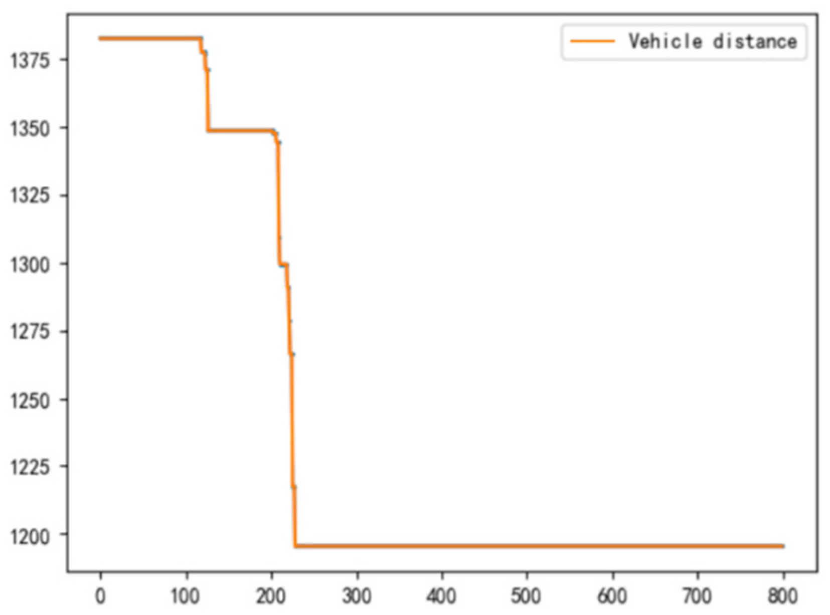
Using the genetic algorithm to solve area routes, the convergence of vehicle routes was obtained. The convergence diagram of vehicle routes in the total area is shown in Figure 2, and solving vehicle routes in the total area is shown in Figure 3. Figure 4 presents a diagram of the shortest path problem for a single vehicle - a single area, where each point represents a service point that needs to be visited.
In the subarea TSP model, the nearest insertion method and genetic algorithm were used to solve the problem, respectively. Under the same running environment, the genetic algorithm only takes 1 min to solve, while the nearest insertion method needs more than 1 h to solve. It can be seen that the nearest insertion method of the TSP for vehicle routing optimization in the Xiaoshun Project was relatively small and slow in data processing. The use of the genetic algorithm provided a large amount of computational data and a fast processing speed. The main solution results of the two algorithms are shown in Table 2.

4.3. Multi-Area Vehicle Transportation Optimization Analysis

For the research on the VRP problem of the Xiaoshun Project, this paper adopted the nearest insertion method and genetic algorithm based on subarea division to solve it. The specific solving process is as follows:
(1) Subarea division. This article used the quadrant-based method to divide subareas. From the perspective of pure theoretical construction, an infinite number of discrete points, through continuous extension or orderly aggregation, form a line with one-dimensional extension. Therefore, the quadrant-based method is not applicable to smaller areas or regions with fewer service points. For instance, residential areas, shopping malls, and factories, which are common service areas, are not suitable for using this zoning method. By using different colors to mark the areas, with pixels of different colors, it is easier for the algorithm to recognize the image, thus improving the accuracy of the recognition. Since before the image recognition, manual processing of necessary points, starting points, coordinate axes, etc., is required, it can also be adjusted in real time according to the actual situation. The annotation information uses blue as the standard horizontal and vertical coordinates, green for the starting point, and red for the necessary points. The specific operation process is as follows: (1) Set the starting point of the vehicle as the origin. Based on the intersection of the two main roads corresponding to the origin, the image is divided into four quadrants by the x-axis and y-axis. (2) To process the image: In the code, red dots are used to mark the edge pixels, blue lines to mark the coordinates, and green dots to mark the center point of the image, which helps the model more accurately identify the relative positions of the coordinates. The image is recognized four times, and the first, second, third, and fourth quadrants are recognized, respectively. When recognizing the fourth quadrant, the upper left corner of the image is taken as the relative origin. (3) To call the cv2 library for coordinate recognition: First, perform edge detection, using the Sobel operator to obtain a binary edge map (edge pixels are 255, background is 0). (4) To extract the coordinates: Traverse each pixel of the edge map and record all pixel coordinates (x, y) (x = column number, y = row number) where the gray value is 255. (5) To calculate the relative positions: Directly use the extracted (x, y) as the relative coordinates from the relative origin (the upper left corner of the image (0, 0)); calculate the center point (cx, cy), where the coordinate of the edge pixel relative to the center point is (x-cx, y-cy); specify a reference pixel (such as the first edge pixel), and the coordinates of other pixels relative to the reference point are (x-ref_x, y-ref_y). Therefore, this example is divided into four subareas according to the actual situation, as shown in Figure 5.
(2) Nearest insertion method. The principle of solving the TSP optimization path after area division is the same as that of solving the optimal path of the total area by using the nearest insertion method above. The analysis process is omitted, and the summary of the minimum mileage of each sub-region is shown in Table 3.
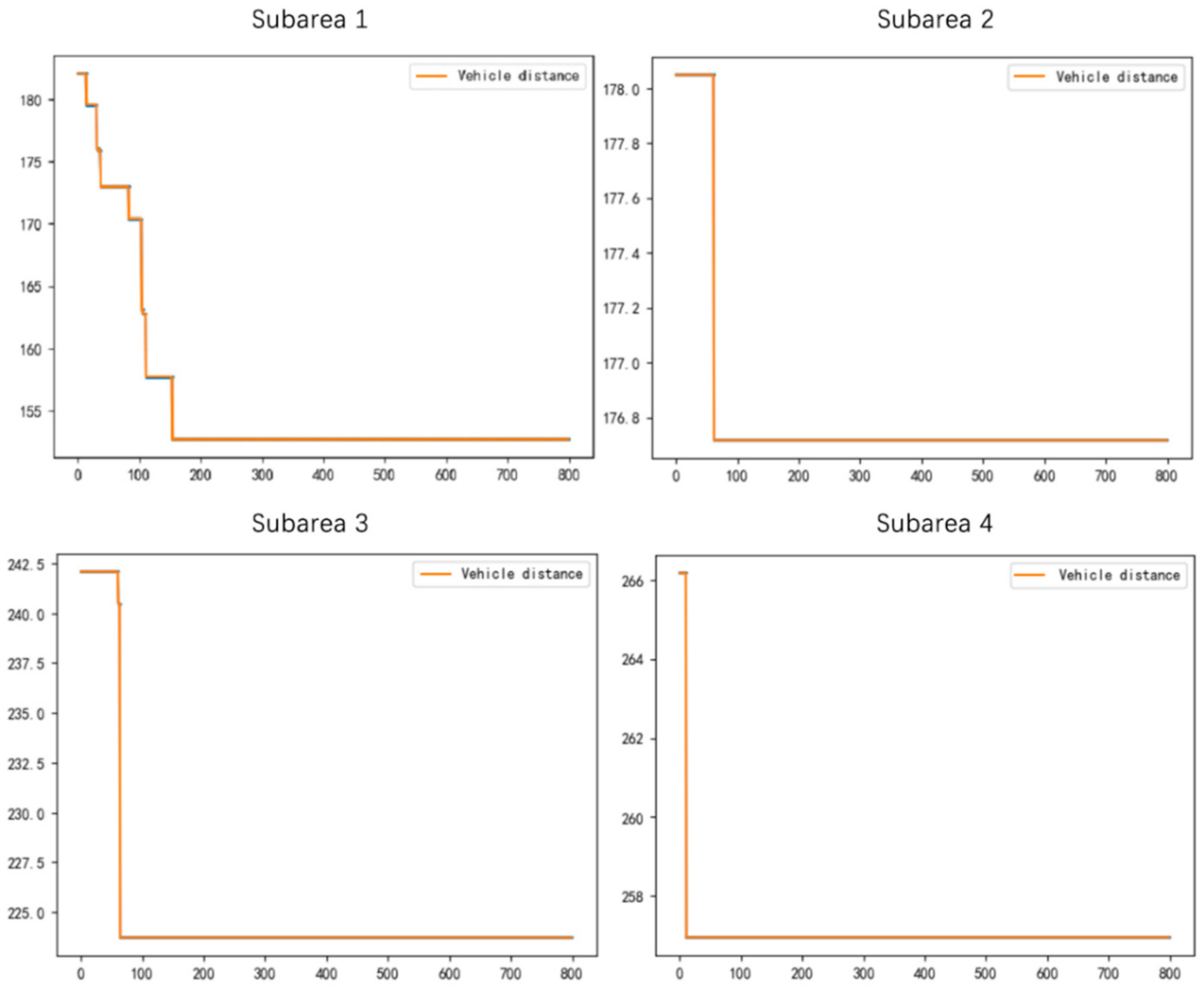
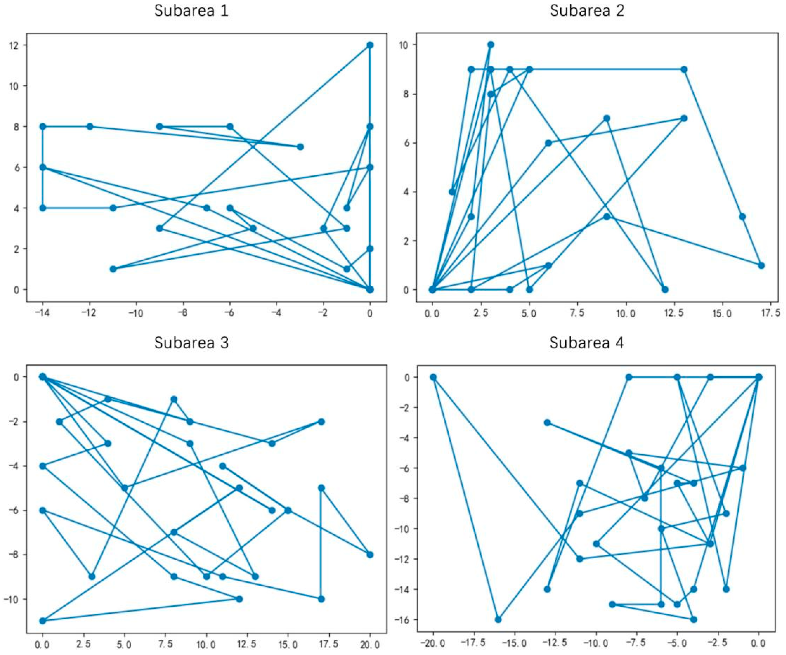
(3) Genetic algorithm. The genetic algorithm is used to solve each subarea route, respectively. The convergence diagram of vehicle routes in each subarea is shown in Figure 6, and the summary for solving vehicle routes in each subarea is shown in Figure 7. The analysis process was omitted, and the summary of the minimum mileage of each subarea is shown in Table 4. Figure 7 presents the diagram of the shortest path problem for four vehicle - subarea, where each point represents a service point that needs to be visited.
In the multi-area VRP model, the nearest insertion method and genetic algorithm were used for comparative analysis. Under the same running environment, the genetic algorithm only takes 2 min to solve, while the nearest insertion method needs more than 3 h to solve. It can be seen that the nearest insertion method of the VRP for vehicle routing optimization in the Xiaoshun Project was relatively small and slow in data processing. The use of the genetic algorithm has a large amount of computational data and a fast processing speed. The main solution results of the two algorithms are shown in Table 5.
(4) Sensitivity analysis. By applying the TSP and VRP algorithms and taking into account the factors such as the number of vehicles, the size of the operation area, and the number of service points, a sensitivity analysis was conducted. The threshold setting for the instance analysis was determined based on the algorithm requirements, combined with expert opinions and the actual situation of the enterprise project as follows: (1) The number of vehicles is determined by the type of algorithm. The TSP is essentially a single-vehicle problem that traverses all service points without a multi-vehicle allocation issue, so the threshold K is directly defined as 1. The VRP is a multi-vehicle problem with no upper limit for its k value and a lower limit of 1. Considering the actual situation of the enterprise, the maximum number of vehicles for a single project is 5, so the threshold for the experimental data is set from 1 to 5. (2) The threshold range for the operational area size is from 10 km2 to 200 km2. We divided the experimental scenarios into three types based on the size of the service area in the industry: the short-distance scenario was set at 10 km2, the medium-distance scenario at 50 km2, and the long-distance scenario at 200 km2, and we conducted experiments for each of the three scenarios. (3) The threshold range for the service points is from 10 to 200. Based on expert opinions, we divided the corresponding scenarios into three problem scales for resolution: the small-scale problem was set at 10, the medium-scale problem at 50, and the large-scale problem at 200. The results are shown in Table 6.
Table 6 illustrates the impact of factors such as the number of vehicles, the size of the operation area, and the number of service points on the TSP and VRP algorithms. For each factor, as its value increased, the corresponding service distance value also increased. This trend demonstrated the robustness of the method proposed in this paper, thereby ensuring its scientific basis for practical applications.

4.4. Comparative Analysis of Vehicle Transportation Costs

The main costs involved in route optimization include vehicle amortization costs, labor costs, and time costs. The vehicle amortization cost needed to take into account the years of purchase and working hours. The formula for calculating the cost of property city service is as follows:
C t o t a l = C f u e l + C w a t e r + C l a b o r + C t i m e
The vehicle consumption cost considers the fuel consumption of single vehicles and multiple vehicles under different mileage conditions, and the mileage consumption cost of single vehicles and multiple vehicles was compared. The daily costs mainly included the costs of vehicle water consumption, fuel, labor and time, etc. The labor cost considers the personnel needs of single areas and multiple areas, and it compares the labor cost according to the personnel needs. Considering the time requirements within the entire operating area, the subarea model scheme is used when time is sufficient, and the multi-area model scheme is arranged when time is tight. Formula (6) can be used to calculate the total cost of the calculation results of the above methods. A summary of various costs calculated by different methods is shown in Table 7.
The research results show that, regardless of whether it is the single-area or multi-area mode, the use of the genetic algorithm saves more costs than the nearest insertion. The total cost of the former was saved by 12.4%, while that of the latter was saved by 21.8%. The multi-area mode saved costs compared to the single-area mode. By using nearest insertion, the total cost was reduced by 35.7%, and by using the genetic algorithm, the total cost was reduced by 42.6%.
The types of algorithms and regional areas, as well as the number of service points, were selected based on relevant numerical simulation tests. To ensure the robustness of the experimental results, the same tests were simulated multiple times to obtain a range of mileage results. This result was used as an indicator for evaluating the optimization of the algorithm’s mileage. By comparing the results of different situations, it was considered that the VRP algorithm is more reasonable, as the repeated driving sections were relatively short. Since the basic data for the case analysis in this paper came from a real project of Limin Environment, the above analysis results have good practical value.

5. Conclusions

This paper provides a path optimization framework based on an intelligent algorithm for the theoretical and applied research of property city service mode. Based on the vehicle route optimization problem in a property city, a route optimization analysis framework combining the nearest insert method and intelligent algorithm was constructed. The feasibility of combining different scenarios and methods was verified through example analysis, and the effectiveness of the intelligent optimization algorithm based on cost comparison analysis was summarized. The example analysis showed that the intelligent algorithm had obvious cost advantage over the nearest insertion method, and the multi-area had obvious cost advantage over the single-area division. The theoretical and practical analysis in this paper showed that the research framework proposed in this paper is feasible. It can be seen that the total cost of using an intelligent algorithm is lower than the total cost of using the nearest insertion method in both single-area and multi-area cases. The total cost in the multi-area case was generally lower than the total cost in the single-area case, the total cost in single-area using the same algorithm was higher than the total cost in the multi-area case, and the total cost in single-area using the intelligent algorithm was higher than the total cost in multi-area using the recent insertion method. Furthermore, the same rules apply to each cost type.
In this study, the intelligent optimization algorithm was applied to the analysis of vehicle routing optimization in a property city, which has reference significance for the theory and practice of property city area operation management. As a new mode of property service, the study of operation optimization of property city has both theoretical and practical value. It should be noted that the above rules do not apply in all cases. When the job area is too small, using a multi-area method is not necessarily the best choice. It is also necessary to consider the influence of cost, which is also the deficiency of this paper. The follow-up research can incorporate other classic methods to conduct more extensive research based on the actual needs of optimizing property city service operations. We can also explore the application of these methods in areas such as IoT, stochastic demand, and multi-objective optimization.

Author Contributions

Conceptualization, J.Y. and W.Z.; methodology, K.F.; software, Y.L.; validation, J.A. and W.Z.; formal analysis, W.Z.; investigation, J.L.; resources, J.L.; data curation, K.F.; writing—original draft preparation, J.Y.; writing—review and editing, J.A. and Y.L.; visualization, L.C.; supervision, J.A. and W.Z.; project administration, J.A. and W.Z.; funding acquisition, W.Z. All authors have read and agreed to the published version of the manuscript.

Funding

This research was funded by [the Provincial and Ministerial-level or Higher-level Scientific Research Cultivation Projects of Zhejiang College of Shanghai University of Finance and Economics] grant number [YJPY202502], [the Anhui Philosophy and Social Science Planning Project] grant number [AHSKQ2019D024], [the Higher School Outstanding Young Talent Support Project of Anhui Province] grant number [GXYQZD2020105] and [2024 annual routine project of Zhejiang Higher Education Association in China] grant number [202428].

Data Availability Statement

The original contributions presented in this study are included in the article. Further inquiries can be directed to the corresponding author.

Conflicts of Interest

Jintao Lin is an employee of Wenzhou Sapphires Property Management Co., Ltd., and Linfeng Chen is an employee of Zhejiang Limin Environmental Technology Co., Ltd. The remaining authors declare that the research was conducted in the absence of any commercial or financial relationships that could be construed as a potential conflict of interest.

References

  1. Niu, G. Hengqin property city mode to achieve intelligent empowerment. People Daily Online, 8 June 2020. [Google Scholar]
  2. Shen, H.; Tu, K.; Chiang, T. Establish a customer property service strategy framework. Int. J. Strateg. Prop. Manag. 2021, 25, 204–215. [Google Scholar] [CrossRef]
  3. Sun, M.; Tan, Y.; Lin, H. Review on the model of property city under the background of urban governance modernization. Housing Real Est. 2023, 9, 12–14. [Google Scholar]
  4. Shen, T.; Zhao, Z.; Wu, X.; Wen, F. Theory and practice of property city--Research on innovative mode of urban governance in Hengqin New District. SSAP 2021, 35–62. Available online: https://xiaoshuo.qq.com/detail/1054865401 (accessed on 21 October 2025).
  5. Huang, Y.H.; Lee, P.C. Role of property management in service demands of elderly residents of apartment complexes. Int. J. Strateg. Prop. Manag. 2020, 24, 1–14. [Google Scholar]
  6. Liao, H.; Jiang, L.; Xu, Z.; Xu, J.; Herrera, F. Herrera, A linear programming method for multiple criteria decision making with probabilistic linguistic information. Inf. Sci. 2017, 415, 341–355. [Google Scholar]
  7. Zeng, S.; Ye, A.; Su, W.; Chen, M.; Llopis-Albert, C. Llopis-Albert, Site evaluation of subsea tunnels with sightseeing function based on dynamic complex MARCOS method. Technol Forecast. Soc. 2024, 199, 123041. [Google Scholar] [CrossRef]
  8. Zhang, N.; Su, W.; Zhang, C.; Zeng, S. Evaluation and selection model of community group purchase platform based on WEPLPA-CPT-EDAS method. Comput. Ind. Eng. 2022, 172, 108573. [Google Scholar]
  9. Liu, Z.; Wang, W.; Liu, P. Dynamic consensus of large group emergency decision-making under dual-trust relationship-based social network. Inf. Sci. 2022, 615, 58–89. [Google Scholar]
  10. Cao, M.; Chiclana, F.; Liu, Y.; Wu, J.; Herrera-Viedma, E. A bilateral negotiation mechanism by dynamic harmony threshold for group consensus decision making. Eng. Appl. Artif. Intell. 2024, 133, 108225. [Google Scholar] [CrossRef]
  11. Zuo, W.; Li, D.; Yu, G. A general multi-attribute multi-scale decision making method based on dynamic LINMAP for property perceived service quality evaluation. Technol. Econ. Dev. Eco. 2020, 26, 1052–1073. [Google Scholar] [CrossRef]
  12. Zuo, W.; Liu, L.; Hu, Q.; Zeng, S.; Hu, Z. A property perceived service quality evaluation method for public buildings based on multisource heterogeneous information fusion. Eng. Appl. Artif. Intell. 2023, 122, 106070. [Google Scholar] [CrossRef]
  13. Dantzig, G.; Ramser, J. The truck dispatching problem. Manag. Sci. 1959, 10, 80–91. [Google Scholar] [CrossRef]
  14. Kim, G.; Ong, Y.; Heng, C.; Tan, P.; Zhang, N. City vehicle routing problem (city VRP): A review. IEEE T. Intell. Transp. 2015, 16, 1654–1666. [Google Scholar] [CrossRef]
  15. Wassan, N. A reactive Tabu search for the vehicle routing problem. J. Oper. Res. Soc. 2006, 57, 111–116. [Google Scholar] [CrossRef]
  16. Xu, Y.; Fang, M.; Chen, L.; Xu, G.; Du, Y.; Zhang, C. Reinforcement learning with multiple relational attention for solving vehicle routing problems. IEEE T. Cybern. 2021, 52, 11107–11120. [Google Scholar] [CrossRef] [PubMed]
  17. Wang, Q.; Hao, Y.; Cao, J. Learning to traverse over graphs with a monte carlo tree search-based self-play framework. Eng. Appl. Artif. Intell. 2021, 105, 104422. [Google Scholar] [CrossRef]
  18. Pérez-Rodríguez, R.; Hernández-Aguirre, A. Simulation optimization for the vehicle routing problem with time windows using a Bayesian network as a probability model. Int. J Adv. Manuf. Tech. 2016, 85, 2505–2523. [Google Scholar] [CrossRef]
  19. Ma, J.; Fang, Y.; Yuan, J. Mutstion ant colony algorithm for multiple-depot multiple-types vehicle routing problems with shortest finfish time. Syst. Eng. Theory Pract. 2011, 31, 1508–1516. [Google Scholar]
  20. Vázquez-Fernández, E.; Coello, C.; Troncoso, F. An adaptive evolutionary algorithm based on typical chess problems for tuning a chess evaluation function. Comput. Ind. Eng. 2012, 62, 306–317. [Google Scholar]
  21. Fayad, C.; Webb, P. Development of a hybrid crisp-fuzzy logic algorithm optimised by genetic algorithms for path-planning of an autonomous mobile robot. Intell. Fuzzy Syst. 2006, 17, 15–26. [Google Scholar] [CrossRef]
  22. Dong, G.; Guo, W.; Tickle, K. Solving the traveling salesman problem using cooperative genetic ant systems. Expert Syst. Appl. 2012, 39, 5006–5011. [Google Scholar] [CrossRef]
  23. Applegate, D.; Bixby, R.; Vaek, C.; Cook, W. The Traveling Salesman Problem: A Computational Study; PUP: Princeton, NJ, USA, 2006. [Google Scholar]
  24. Bouhmala, N. A multilevel genetic algorithm for the traveling salesman problem. ENDM 2003, 15, 54. [Google Scholar] [CrossRef]
  25. Srivastava, G.; Singh, A. Two evolutionary approaches with objective-specific variation operators for vehicle routing problem with time windows and quality of service objectives. Appl. Soft Comput. 2023, 134, 109964. [Google Scholar] [CrossRef]
  26. Tutumlu, B.; Sarac, T. A mip model and a hybrid genetic algorithm for flexible job-shop scheduling problem with job-splitting. Comput. Oper. Res. 2023, 155, 106222. [Google Scholar] [CrossRef]
  27. Le, M.; Nguyen-Duy-Nhat, V.; Nguyen, H.; Shin, O. Ddpg-based optimization for zero-forcing transmission in uav-relay massive mimo networks. IEEE Open J. Commun. Soc. 2024, 4, 3386595. [Google Scholar] [CrossRef]
  28. Goldberg, D. Genetic Algorithms in Search, Optimization, and Machine Learning; Addison-Wesley Longman Publishing Co., Inc.: Boston, MA, USA, 1989. [Google Scholar]
  29. Talbi, H.; Draa, A.; Batouche, M. A new quantum-inspired genetic algorithm for solving the travelling salesman problem. IEEE 2004, 3, 1192–1197. [Google Scholar]
  30. Uthayasuriyan, A.; Hema, C.; Kavvin, U.; Mahitha, S.; Jeyakumar, G. A comparative study on genetic algorithm and reinforcement learning to solve the traveling salesman problem. RRCS 2023, 2, 1–12. [Google Scholar] [CrossRef]
  31. Yusuf, I.; Baba Mohd, S.; Iksan, N. Applied genetic algorithm for solving rich VRP. Appl Artif Intell. 2014, 28, 957–991. [Google Scholar] [CrossRef]
  32. Vaira, G.; Kurasova, O. Genetic algorithm for vrp with constraints based on feasible insertion. Informatica 2014, 25, 155–184. [Google Scholar] [CrossRef]
  33. Wang, S.; Huang, Q. A hybrid code genetic algorithm for vrp in public-private emergency collaborations. Int. J. simul. Model 2022, 21, 124–135. [Google Scholar] [CrossRef]
  34. Rosenkrantz, D.; Stearns, R.; Lewis, P. An analysis of several heuristics for the traveling salesman problem. Siam. J. Comput. 1977, 6, 563–581. [Google Scholar] [CrossRef]
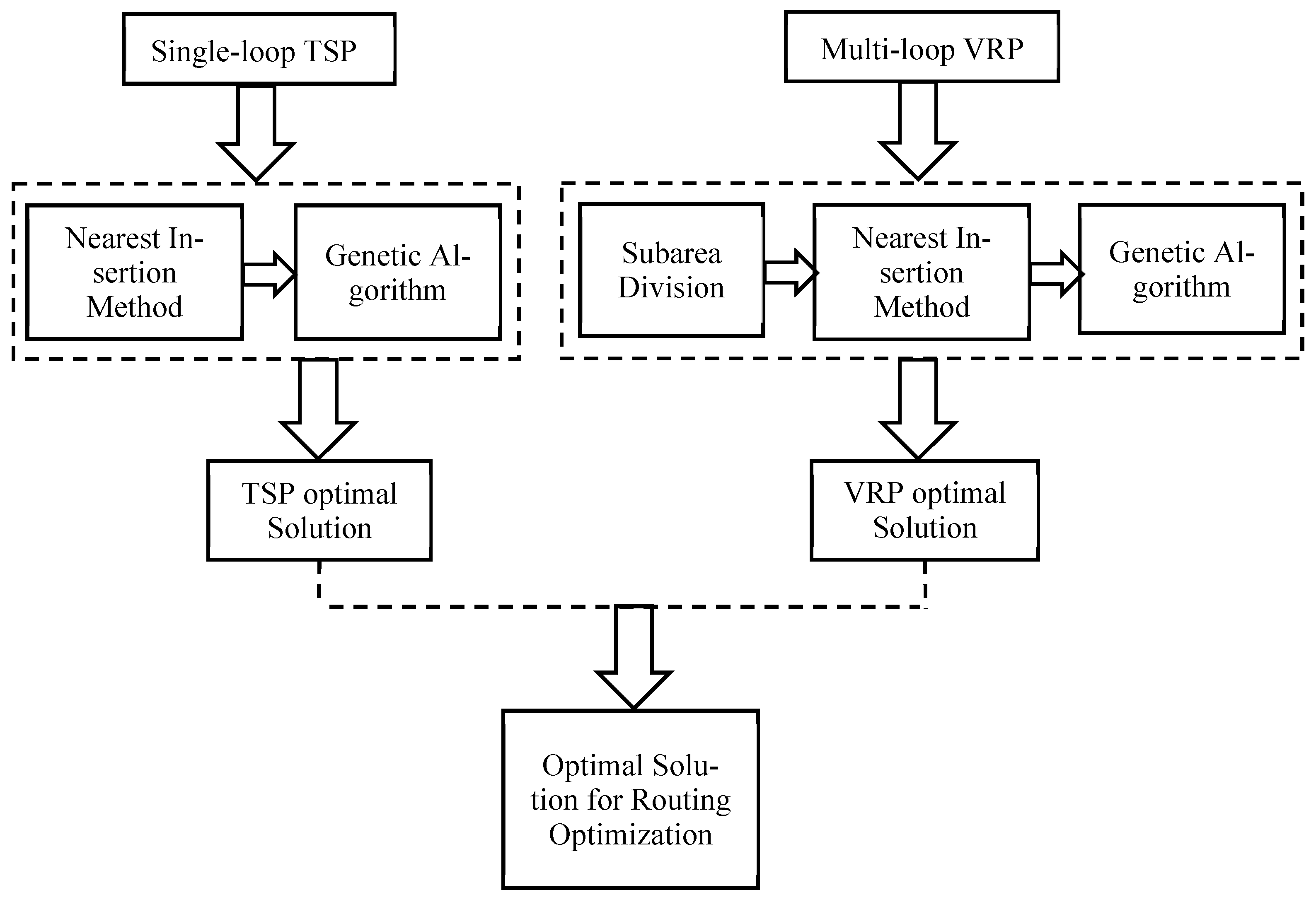
Figure 1. Frame diagram of vehicle routing optimization analysis.
Wevj 17 00025 g001
Figure 2. Description of the genetic algorithm.
Wevj 17 00025 g002
Figure 3. The convergence diagram of vehicle routes.
Wevj 17 00025 g003
Figure 4. Vehicle routes diagram.
Wevj 17 00025 g004
Figure 5. Area division of Xiaoshun Town.
Wevj 17 00025 g005
Figure 6. Convergence diagram of vehicle routes in each subarea.
Wevj 17 00025 g006
Figure 7. Solving route diagram of vehicle routes in each subarea.
Wevj 17 00025 g007
Table 1. Summary of unit prices of each cost.
Cost TypeUnit Price
Running fuel consumption7.5 yuan/L
Fuel per kilometer0.5 L/km
Water price1.5 yuan/ton
Water per kilometer0.8 tons/km
Labor cost30 yuan/h
Time cost50 yuan/h
Table 2. Comparison of TSP solution results in a single area.
Solution ResultNearest Insertion MethodGenetic Algorithm
Minimum mileage (km)135.2119.5
Oil consumption (L)67.659.8
Time required (hours)6.75.8
Water consumption (tons)108.195.6
Table 3. Summary of subarea mileage by use of nearest insertion method.
ItemsMileage (km)
Subarea 117.27
Subarea 218.21
Subarea 322.96
Subarea 428.51
Total area mileage86.95
Table 4. Summary of subarea mileage by use of genetic algorithm.
ItemsMileage (km)
Subarea 114.24
Subarea 213.26
Subarea 320.04
Subarea 421.55
Total area mileage69.10
Table 5. Comparison of VRP solution results in multiple areas.
Solution ResultNearest InsertionGenetic Algorithm
Minimum mileage (km)87.0 69.1
Oil consumption (L)43.5 29.9
Time required (hours)4.3 3.3
Water consumption (tons)69.6 55.3
Table 6. Results of sensitivity analysis.
Algorithm TypeNumber of VehiclesArea Size of OperationNumber of Service Points
1050200
TSP
(single vehicle)
1 vehicle10 km212.8~15.3 km38.5~45.2 km102.6~123.5 km
50 km228.6~33.5 km85.7~98.3 km228.4~265.9 km
200 km257.2~67.1 km171.3~196.7 km456.8~531.8 km
VRP
(multiple vehicles)
2 vehicles10 km28.3~10.5 km24.6~29.1 km65.8~78.3 km
50 km218.5~22.3 km55.2~64.1 km146.8~172.5 km
200 km237.0~44.5 km110.5~128.2 km293.6~345.0 km
3 vehicles10 km26.5~8.2 km18.9~23.3 km50.2~61.4 km
50 km214.5~17.8 km42.5~51.3 km113.2~135.7 km
200 km229.0~35.6 km85.0~102.6 km226.4~271.4 km
5 vehicles10 km25.8~7.5 km15.3~19.6 km39.8~49.7 km
50 km212.8~16.1 km34.6~42.7 km90.5~112.3 km
200 km225.6~32.2 km69.2~85.4 km181.0~224.6 km
Table 7. Different methods of calculating each cost (unit: yuan).
Cost TypeSingle-Area CostMulti-Area Cost
Nearest InsertionGenetic AlgorithmNearest InsertionGenetic Algorithm
Fuel cost507.0448.1326.3259.1
Water cost162.2143.4104.482.9
Labor cost201.0174.0129.099.0
Time cost335.0290.0215.0165.0
Total cost1205.21055.5774.65606.0
Disclaimer/Publisher’s Note: The statements, opinions and data contained in all publications are solely those of the individual author(s) and contributor(s) and not of MDPI and/or the editor(s). MDPI and/or the editor(s) disclaim responsibility for any injury to people or property resulting from any ideas, methods, instructions or products referred to in the content.