Prediction of Motor Rotor Temperature Using TCN-BiLSTM-MHA Model Based on Hybrid Grey Wolf Optimization Algorithm

Abstract

The permanent magnet synchronous motor (PMSM) is the core of new energy vehicle drive systems, and its temperature status is directly related to the safety of the entire vehicle. However, the temperature of rotor permanent magnets is difficult to measure directly, and traditional sensor schemes are costly and complex to deploy. With the development of Artificial Intelligence (AI) technology, deep learning (DL) provides a feasible path for sensorless modeling. This paper proposes a prediction model that integrates a Temporal Convolutional Network (TCN), Bidirectional Long Short-Term Memory Network (BiLSTM), and multi-head attention mechanism (MHA) and introduces a Hybrid Grey Wolf Optimizer (H-GWO) for hyperparameter optimization, which is applied to PMSM temperature prediction. A public dataset from Paderborn University is used for training and testing. The test set verification results show that the H-GWO-optimized TCN-BiLSTM-MHA model has a mean absolute error (MAE) of 0.3821 °C, a root mean square error (RMSE) of 0.4857 °C, and an R² of 0.9985. Compared with the CNN-BiLSTM-Attention model, the MAE and RMSE are reduced by approximately 11.8% and 19.3%, respectively.

1. Introduction

The permanent magnet synchronous motor (PMSM) is widely used in industrial, transportation, and new energy fields due to its high efficiency, high torque density, and excellent control performance. Since its internal permanent magnets are highly sensitive to temperature, excessive temperature may lead to insulation failure and magnetic performance degradation, affecting operating efficiency and service life. Therefore, accurate prediction of rotor temperature is of great significance for improving system performance and reducing energy consumption and risks. However, due to the high-speed rotation of the rotor permanent magnets inside the motor and the complexity of the rotor structure, it is difficult to arrange sensors, which also increases costs and potential safety hazards [1,2].

Traditional temperature prediction methods mainly include three types: Computational Fluid Dynamics (CFD), Finite Element Analysis (FEA), and Lumped-Parameter Thermal Network (LPTN) [3,4]. Dong et al. used CFD modeling to evaluate the temperature distribution of high-speed permanent magnet motors [5]. Sun et al. applied 2-D finite element analysis to estimate the temperature rise in motor rotors [6]. However, CFD and FEA are constrained by the ideal conditions of modeling and the accuracy of models. Moreover, they involve complex calculations and consume substantial computing resources, thus making them generally unsuitable for temperature monitoring with real-time requirements [7]. The LPTN method is an approach used to build an equivalent network model based on thermodynamics theory [8,9]; it has a faster calculation speed than CFD and FEA, but due to the complexity of the PMSM’s structure and materials, the LPTN model may fail to capture the detailed distribution of the thermal field.

In recent years, Physics-Informed Neural Networks (PINNs), as hybrid methods integrating deep learning and physical principles, have begun to be applied in the field of real-time thermal prediction [10]. However, in the scenario of motor rotor temperature prediction, PINNs have two key limitations. First, they rely heavily on accurate prior physical equations and precise quantification of physical parameters. During the actual operation of the motor, variable operating conditions, such as sudden load changes and transient speed changes, will cause physical parameters to vary with time, resulting in a mismatch between the fixed physical constraints in PINNs and the actual operating conditions [11]. Second, the embedding of physical constraints increases the model complexity of the PINN [12]. When processing the same motor temperature dataset, PINNs require more training time than data-driven deep learning models, which weakens their real-time advantage in on-board applications.

Classic deterministic methods for time series have long been applied in the field of temperature prediction. The Autoregressive Integrated Moving Average (ARIMA) model captures linear temporal dependencies by combining Autoregressive (AR) and Moving Average (MA) components, but it is unable to handle nonlinear relationships in motor rotor temperature [13]. Exponential smoothing models (such as the Holt–Winters model) predict future values by assigning exponentially decreasing weights to historical data; however, they are sensitive to outliers in temperature data and cannot capture long-term temporal correlations [14]. These limitations have prompted researchers to adopt deep learning techniques—which offer greater advantages in nonlinear feature extraction and long-sequence modeling—for motor rotor temperature prediction.

By contrast, deep learning (DL), leveraging its robust nonlinear modeling capability and data-driven nature, has demonstrated significant advantages in temperature prediction. Typical DL networks, represented by DNNs, LSTM, and CNNs, do not rely on explicit physical equation constraints, thus avoiding errors caused by incomplete physical assumptions. They can achieve efficient and accurate temperature estimation solely based on operating data such as current, voltage, and rotational speed. Meanwhile, they possess characteristics including excellent real-time performance, high cost-effectiveness, and strong adaptability, making them more aligned with the practical requirements of motor rotor temperature monitoring [1,15,16,17,18,19,20].

In the field of time-series modeling, various deep learning techniques exhibit different modeling advantages based on their unique network structure designs, providing diverse technical pathways for motor temperature prediction. Long Short-Term Memory (LSTM) networks address the gradient vanishing problem of the traditional recurrent neural network (RNN) through a gating mechanism. They can effectively capture the long-term temporal dependencies of dynamic systems, making them particularly suitable for temperature sequence prediction involving complex transient features. Temporal Convolutional Networks (TCNs) adopt a dilated convolution structure, which can flexibly expand the receptive field by adjusting the dilation coefficient. While maintaining computational efficiency, TCNs capture multi-scale local temporal features, and their parallel computing capability is significantly superior to that of recurrent neural networks. Differential Feedforward Neural Networks (DFNNs) enhance the ability to model the rate of change in input features by introducing differential operators, demonstrating unique advantages in handling the nonlinear mapping relationship between motor operating parameters and temperature. Convolutional Neural Networks (CNNs) leverage the local receptive field and weight sharing mechanism to efficiently extract spatial correlation features from temperature sequences. Bidirectional Long Short-Term Memory (BiLSTM) networks utilize hidden layer structures in both forward and backward directions, enabling them to simultaneously capture the impact of future states on current temperatures. This makes BiLSTM more suitable for modeling bidirectional temporal processes such as motor start-up and shutdown.

The aforementioned technologies have been validated in the field of PMSM temperature prediction, and the relevant research findings provide important references for subsequent technical optimization. Oliver Wallscheid et al. [17] were the first to apply LSTM to PMSM temperature time-series prediction, using a particle swarm optimization algorithm to search for the optimal hyperparameters of the model. However, this optimization method evaluates each candidate solution in the search space only once, making it difficult to fully traverse the global optimal domain, which limits the hyperparameter optimization accuracy to a certain extent. The TCN model constructed by Wilhelm Kirchgässner et al. [1] achieved a mean squared error (MSE) of 3.04. Compared with the traditional RNN, this validates its efficiency in motor temperature series modeling. The Deep Feedforward Neural Network-Nonlinear AutoRegressive with eXogenous inputs (DFNN-NARX) model proposed by Jun Lee et al. [18] demonstrates significantly better performance than traditional feedforward neural networks in the temperature estimation of stator windings and permanent magnets. Hosseini et al. [19] compared the prediction effects of CNNs and LSTM and found that CNNs are more effective in predicting the temperatures of stators and rotor permanent magnets, achieving an MSE of 2.64 and an average coefficient of determination (R²) of 0.9924. Mohammed Bouziane et al. [20] used a recurrent neural network with BiLSTM units to model the complex relationships of motor parameters; the R² score of temperature prediction on the test set reached 0.99, confirming its modeling accuracy for nonlinear correlations.

Numerous studies have confirmed the effectiveness of the attention mechanism in time-series forecasting. Wang and Zhang [21] proposed a multi-stage attention network: they leveraged the attention mechanism to capture the differential impacts of non-forecast sequences on target sequences, incorporated a score adjustment module to avoid the omission of key information, and combined a gated recurrent unit (GRU)-based LSTM network to enhance the capture of abrupt change information, with convergence optimized via the AdaHMG algorithm. When tested on the Nasdaq100 and PM2.5 datasets, the mean absolute error (MAE) and root mean square error (RMSE) of this network were reduced by 10.16–33.01% and 12.81–37.55%, respectively, compared with those of the dual-stage attention-based recurrent neural network (DA-RNN). Notably, the more non-forecast sequences there were, the more significant this advantage became. To address the high-dimensionality and nonlinearity issues of multivariate time-series data, Cheng et al. proposed the dual attention-based bidirectional long short-term memory (DABi-LSTM). This model uses input attention to screen key driving sequences, employs BiLSTM to bidirectionally extract temporal features, and integrates LSTM to optimize long-term dependency learning, thereby forming a collaborative architecture [22]. In convolutional-based temporal modeling, Wang and Zhang [21] adapted the temporal attention mechanism to the time dimension: they convolved the output of each layer of the TCN, generated dynamic weights through sigmoid mapping, and achieved performance improvements. Compared with LSTM and GRU, the RMSE and MAE of this modified model were reduced by an average of 10–37%; compared with the basic TCN, these metrics were further reduced by 0.8–10%, breaking the limitation of the “fixed receptive field” in traditional convolution.

Studies by Oliver Wallscheid [17], Wilhelm Kirchgässner [1], Mohammed Bouziane [20], and others have shown that TCNs and BiLSTM exhibit excellent performance in time-series modeling. However, existing research also indicates that single deep learning methods have limited performance under complex operating conditions [23,24], and there is an urgent need to further improve model performance.

To solve the above problems, this paper proposes a TCN-BiLSTM-MHA prediction model based on a Hybrid Grey Wolf Optimization (H-GWO) algorithm. The model comprehensively utilizes the TCN to extract local time-series features, BiLSTM to capture bidirectional dependencies in sequences, and multi-head attention (MHA) to model the importance of different time steps of multi-dimensional information, thereby realizing in-depth mining of the relationship between rotor temperature and other features. At the same time, the H-GWO algorithm is introduced to optimize the model hyperparameters to improve the overall prediction accuracy and generalization ability.

The main contributions of this paper are as follows:

• A hybrid prediction model integrating a TCN, BiLSTM and MHA is proposed, which achieves good experimental results in motor rotor temperature prediction.
• A Hybrid Grey Wolf Optimization algorithm combining Tent chaotic mapping and differential evolution is used to optimize the key parameters of the prediction model, including the number of TCN channels, the number of neurons in BiLSTM hidden layers, and the learning rate, effectively improving the prediction performance of the model.
• Ablation experiments and comparative experiments are carried out on public datasets, verifying the feasibility of the proposed model for rotor temperature prediction and providing a new idea for non-contact prediction of motor rotor temperature.

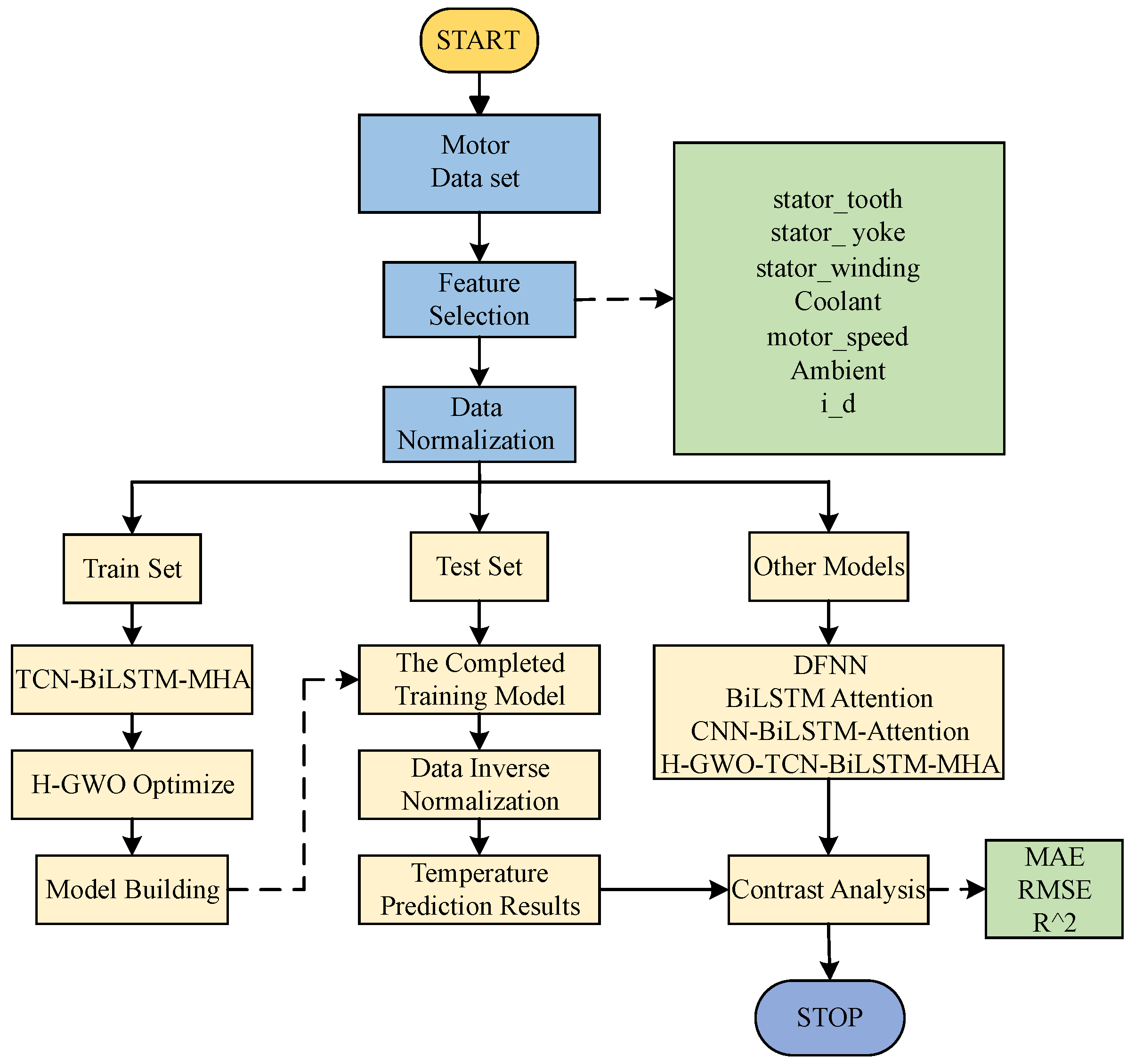
The overall framework of the paper is shown in Figure 1. The paper uses a public motor dataset, selects appropriate input features, and divides the training set and test set in proportion. Then, the training set is input into the constructed temperature prediction model for training, and the model parameters are optimized by H-GWO. After that, the test set is fed into the trained model to finally obtain the prediction results for temperature data. Finally, the model is compared and analyzed with the DFNN, BiLSTM-Attention, and CNN-BiLSTM-Attention models to prove the advantages of the H-GWO-TCN-BiLSTM-MHA model.

2. TCN-BiLSTM-MHA Rotor Temperature Prediction Model

To address the issues of insufficient prediction accuracy and generalization ability of the standalone TCN or BiLSTM model, this paper constructs a composite model integrating time-series modeling, feature extraction, and a multi-head attention mechanism, namely, TCN-BiLSTM-MHA, from three aspects: input feature selection, model structure design, and parameter optimization strategies. Its structure is shown in Figure 2. Firstly, through normalization and feature correlation analysis, the model inputs are ensured to be representative and stable, improving the modeling quality from the source. Secondly, by combining the TCN with BiLSTM, the TCN uses a one-dimensional convolutional structure to effectively extract important features within local time windows while maintaining good parallelism. This enhances the ability to model long-term dependent information and avoids the gradient vanishing problem in traditional recurrent neural networks. On this basis, the bidirectional recurrent structure of BiLSTM is introduced to fully explore the correlation of temperature changes in the time series, improving the model’s ability to perceive global dynamic features. Finally, since the TCN and BiLSTM have a limited ability to model the importance of different time steps and feature dimensions, which may lead to insufficient information utilization, MHA is introduced to weight the high-dimensional sequence representations extracted by BiLSTM, thereby highlighting the time points and feature channels that are more critical to the prediction task.

The combination of the TCN, BiLSTM, and MHA achieves hierarchical optimization from local feature extraction to temporal dependency modeling and then to key feature attention, significantly enhancing the model’s ability to predict rotor temperature under multi-variable and complex operating conditions. This effectively overcomes the shortcomings of single models in temporal modeling and feature weight allocation.

2.1. Temporal Convolutional Network

TCNs have shown certain advantages in multiple sequence data modeling tasks [25], and their advantages stem from causal convolution operations. 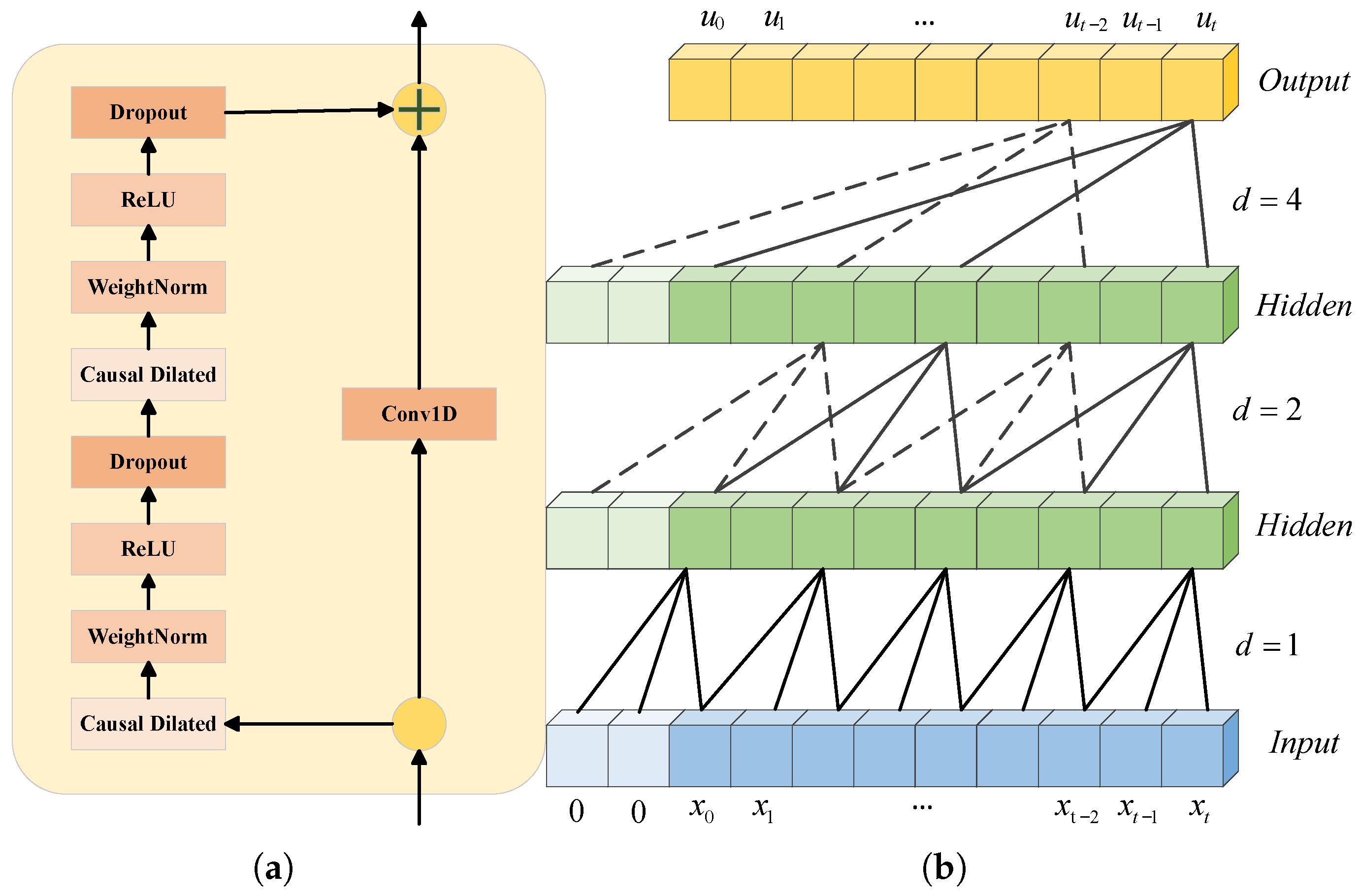The causal convolution of the TCN appropriately pads the input data on the basis of one-dimensional convolution operations so that the input sequence $x_0,\dots ,x_t$ corresponds to the output sequence $u_0,\dots ,u_t$, and the predicted value at time t can only be related to the input values at time t and before t. In addition, the TCN incorporates dilated convolution, where the convolution kernel performs jump sampling on the input sequence, expanding the receptive field in a hierarchical manner and covering longer dependencies with fewer layers. The causal convolution structure of the TCN is illustrated in Figure 3a. Moreover, residual connection is an effective approach for the TCN to transmit information across layers. By leveraging the connectivity of residual blocks, connecting multiple residual blocks can effectively mitigate the gradient explosion issue and expand the model’s receptive field [26]; the structure of the residual block is presented in Figure 3b. The operation of the dilated causal convolution of the TCN on the convolution kernel $f=\left\{f\right(0),\dots ,f(i),\dots ,f(k-1\left)\right\}$ is shown in the following equation:

$$u_t=\sum _i^{k-1}f\left(i\right)·x_{t-d·i}$$

(1)

where $t-d·i$ guides the past direction, and $x_{t-d·i}$ is the input time series; d is the dilation factor; k is the size of the filter; and $f\left(i\right)$ represents the $i-th$ convolution weight.

The input layer feeds time-series data into the TCN layers through sliding windows. Each TCN layer includes convolution, normalization, and ReLU activation operations. The four TCN layers are connected via residual links, each employing one-dimensional convolution with a kernel size of 5 and different dilation rates (1, 2, 4, 8). This allows the TCN layers to model the historical accumulation of rotor temperature rise and the changing trends of operating conditions, achieving multi-dimensional local feature extraction.

2.2. Bidirectional Long Short-Term Memory

BiLSTM is an improved recurrent neural network based on LSTM. By introducing input gates, forget gates, and output gates, it overcomes the problems of gradient vanishing and gradient explosion in RNNs [27]. It can regulate the information flow by retaining important information and deleting irrelevant information, thus realizing the extraction of long-time-series information [27]. The calculation equations for the input gate, forget gate, and output gate that constitute the LSTM unit are shown in (2):

$$\left\{\begin{array}{c}{f}_t=\sigma (W_f·[h_{t-1},u_t]+b_f)\hfill \\ g_t=\sigma (W_g·[h_{t-1},u_t]+b_g)\hfill \\ m_t=tanh(W_m·[h_{t-1},u_t]+b_m)\hfill \\ C_t=f_t\ast C_{t-1}+g_t\ast m_t\hfill \\ n_t=\sigma (W_n·[h_{t-1},u_t]+b_n)\hfill \\ h_t=n_t\ast tanh\left(C_t\right)\hfill \end{array}\right.$$

(2)

where $\{u_0,u_1,\dots ,u_t\}$ represent the input sequence from the LSTM layer; $\sigma$ represents the sigmoid activation function; $f_t$ is the output vector of the forget gate at time t; $W_f$ and $b_f$ are the weight matrix and bias vector of the forget gate; $g_t$ is the output vector of the input gate at time t; $W_g$ and $b_g$ are the weight matrix and bias vector of the input gate; $C_t$ represents the information stored in the state unit at time t; $n_t$ is the output value of the output gate; $h_t$ represents the output value of the state unit at time t; and $W_n$ and $b_n$ are the weight matrix and bias vector of the output gate.

BiLSTM integrates two complementary LSTM structures: one advances along the time axis in the forward direction, simulating the information flow from the past to the present; the other proceeds in the reverse direction, from the future to the past, capturing the impact of future information on the current moment. For the input sequence $\{u_0,\dots ,u_t\}$, where $u_t\in {\mathbb{R}}_{batch\_size\times 128}$, BiLSTM captures bidirectional dependencies in the sequence and obtains a forward sequence $h^{\prime }=\{h_0^{\prime },h_1^{\prime },\dots ,h_t^{\prime }\}$ and reverse sequence $h^{″}=\{h_0^{″},h_1^{″},\dots ,h_t^{″}\}$. The final output sequence $H=\{H_0,H_1,\dots ,H_t\}$, $H\in {\mathbb{R}}_{batch\_size\times seq\_length\times 128}$, is obtained by the following equation:

$$H_t=w_t^{\prime }{h}_t^{\prime }+w_t^{″}{h}_t^{″}+b_t$$

(3)

where $w_t^{\prime }$ and $w_t^{″}$ are weights, and $b_t$ is bias.

2.3. Multi-Head Attention Mechanism

The attention mechanism is a computational model that simulates human visual and cognitive processes. It was initially introduced in machine translation tasks to address the problem of long-distance dependencies. In recent years, the attention mechanism has been extensively researched and applied in the field of deep learning, and it has been applied to various domains, such as natural language processing, computer vision, audio and video processing, etc. [28]. Whether in sequence data or spatial data, the attention mechanism can effectively capture key information, quickly extract more effective information from a large amount of information, and reduce the impact of invalid information on the model training effect [29].

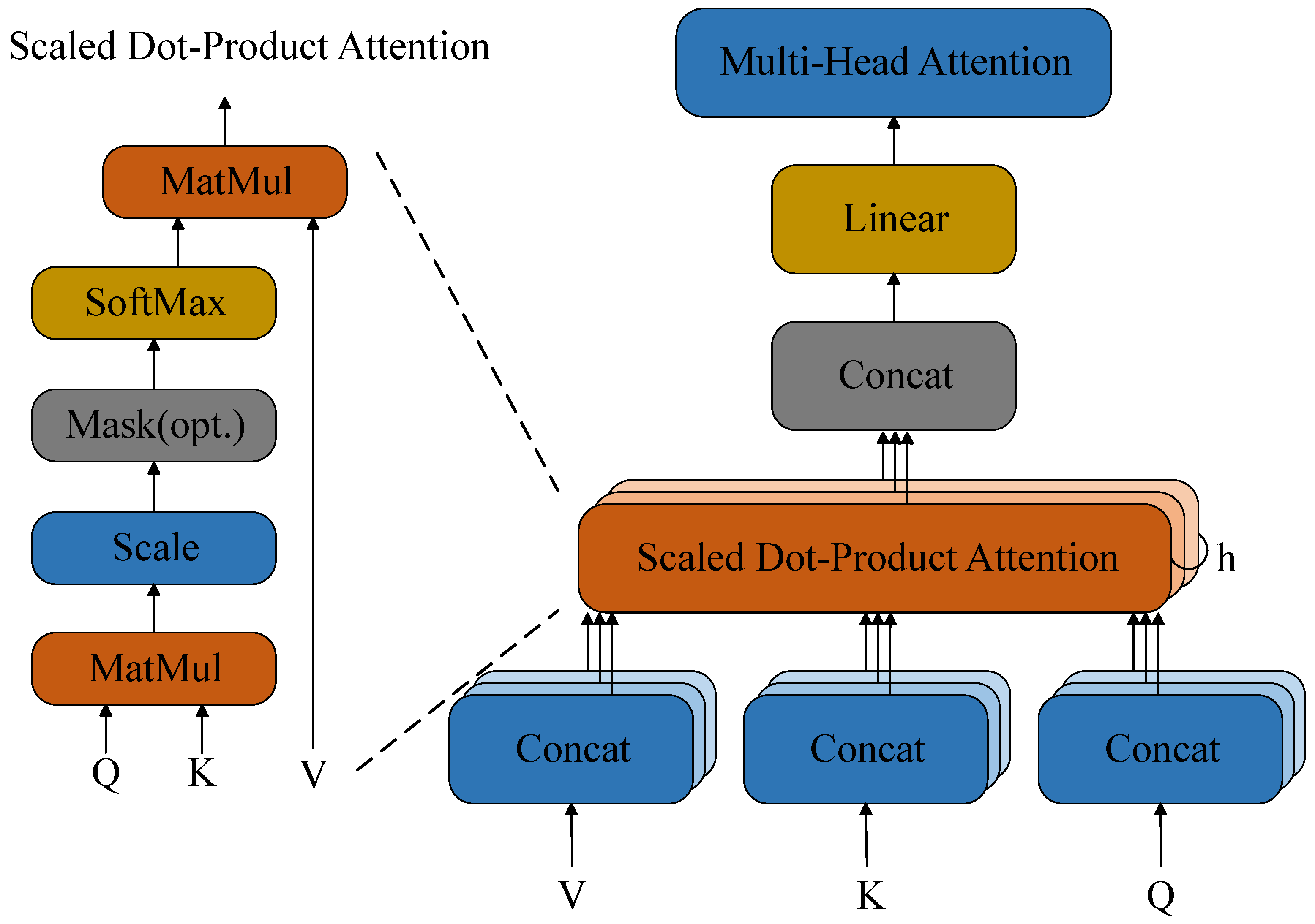
MHA is a combination of multiple self-attention structures [30], as shown in Figure 4. Compared with the single-head attention mechanism, different heads can focus on different patterns and extract more abundant information. In this paper, MHA is set with eight attention heads, which divide the original features into eight subspaces. First, three groups of linear transformations are performed on the input sequence in the feature dimension, with each head processing 16-dimensional data, as shown in Equation (4), to obtain the corresponding Query (Q), Key (K), and Value (V) vectors. Then, after the input features are projected into low-dimensional subspaces, the attention distributions are calculated in parallel within different subspaces, as shown in Equation (5). Subsequently, the attention outputs of all heads are concatenated in the feature dimension and fused through a linear transformation to generate the final multi-head attention output sequence, as shown in Equation (6), resulting in the final output $M\in {\mathbb{R}}_{batch\_size\times seqlength\times 128}$.

$$Q_i=H_i{W}_i^Q,K_i=H_i{W}_i^K,V_i=H_i{W}_i^V$$

(4)

$${Attention}_i(Q_i,K_i,V_i)=softmax\left({\displaystyle \frac{Q_i{K}_i^{\mathrm{T}}}{\sqrt{d_k}}}\right)V_i$$

(5)

$$M=Concat({Attention}_1,{Attention}_2,\dots ,{Attention}_8)W^C$$

(6)

$i=\{1,2,\dots ,8\}$ represents the i-th attention head; the input sequence of the i-th head is $H_i\in {\mathbb{R}}_{batch\_size\times seq\_length\times d}$, where $d=16$ denotes the dimension of the input vector for each head. $W_i^Q,W_i^K,W_i^V\in R_{d\times d_k}$ are three weight matrices, and $d_k=16$ indicates the size of the feature dimension for each head. $W^C\in R_{h\times d\times d_k}$ represents the weight matrix, and $h=8$ denotes the number of heads.

2.4. Output Module

To convert the temporal features from the multi-head attention mechanism into the final temperature prediction values, an output module consisting of an adaptive average pooling layer, a Dropout layer, and a fully connected layer is designed at the end of the model.

First, an average pooling operation is used to compress the sequence data $M=\{m_0,m_1,\dots ,m_t\},m_t\in {\mathbb{R}}_{batch\_size\times 128}$ output by the attention mechanism in the temporal dimension, averaging the features of different time steps to obtain a fixed-length sequence representation:

$$M_{avg}={\displaystyle \frac{1}{t+1}}\sum _{i=0}^t{m}_i$$

(7)

To enhance the generalization ability of the model and prevent overfitting, a Dropout operation is employed to randomly discard some neurons from the pooled feature vector:

$$M_{drop}=Dropout\left(M_{avg}\right)$$

(8)

Finally, a linear fully connected layer is used to map the processed features to the final temperature prediction value:

$$y=W·M_{drop}+b$$

(9)

where W represents the weight matrix, and b represents the bias vector.

2.5. Module Integration

In this study, the TCN, BiLSTM, and MHA models are integrated in a sequential and complementary manner to process the temperature time series of the motor rotor. During model operation, 64 windowed data samples are input per batch (batch_size), with each window having a data length (seq_length) of 64 and a feature dimension of 7; the time step of the sliding window is set to 1. The model starts with four cascaded TCN modules, each using a convolution kernel of size 5, with dilation factors of 1, 2, 4, and 8, respectively. The input data is fed through these four TCN modules sequentially, and the feature dimension of the output data from the last TCN module is mapped to 128, resulting in a sequence data output with the shape ${\mathbb{R}}_{batch\_size\times seq\_length\times 128}$. Subsequently, the local feature map extracted by the TCN is input into the BiLSTM module. Each of the two LSTM layers in the BiLSTM is configured with 64 neurons, which process the 64-time-step data from the TCN in both forward and backward directions. This processing by BiLSTM yields a sequence data output maintaining the shape ${\mathbb{R}}_{batch\_size\times seq\_length\times 128}$. Finally, the data is input into the MHA module. The MHA layer assigns weights to the correlations between the current time step and other time steps, and its output is a weighted key feature sequence with the shape ${\mathbb{R}}_{batch\_size\times seq\_length\times 128}$—this sequence highlights information critical to temperature prediction. Eventually, the average pooling layer compresses the time dimension to 1, and the fully connected layer compresses the feature dimension to 1, generating 1 final predicted value for each time window.

3. Parameter Optimization Algorithm H-GWO Based on Chaos Map and Differential Evolution

In the task of motor rotor temperature prediction, model parameters directly affect the model’s ability to extract time-series features and the final prediction accuracy, such as sequence length, batch size, and number of convolution channels. Traditional methods such as manual empirical parameter tuning or grid search have problems such as low efficiency, difficulty in dimension expansion, and ease in trapping in local optima, which make it difficult to meet the optimization needs of complex model structures in practical engineering. To this end, this paper introduces the Grey Wolf Optimizer (GWO) to automatically search for and optimize the key hyperparameters of the model. The GWO is a swarm intelligence optimization algorithm that simulates the hunting behavior of grey wolf populations. Compared with other optimization algorithms [31,32], it has a stronger global search ability in dealing with problems with less gradient information, nonlinearity, and non-convex optimization. It is particularly suitable for deep learning models with complex parameter spaces and large computational overhead, such as TCN-BiLSTM-MHA.

This algorithm simulates the wolf pack in nature and sets up a four-level pyramid hierarchical structure consisting of $\alpha ,\beta ,\delta ,$ and $\omega$ (current optimal solution, suboptimal solution, third optimal solution, and the remaining individuals), including three hunting behaviors: tracking, encircling, and attacking prey [33,34]. The application of the GWO algorithm in many fields has proven to have great advantages, but it still has drawbacks, such as being prone to falling into local optima and having slow convergence speed and low precision. To address this, Yukun Zheng et al. [35] proposed an improved hybrid GWO (H-GWO) algorithm, which introduces the mutation and crossover strategies of the differential evolution (DE) algorithm and further combines the opposition-based learning technology to overcome the problems of the standard GWO, such as being prone to falling into local optima and insufficient population diversity. The block diagram of the H-GWO algorithm is shown in Figure 5.

3.1. Population Initialization Based on Tent Map and Opposition-Based Learning

According to the set random value ${\theta }_{0,j}$, a chaotic sequence $\left\{{\theta }_{i,j}\right\}$ is recursively generated using the Tent chaotic mapping method:

$${\theta }_{i,j}=\left\{\begin{array}{cc}{\theta }_{i-1,j}/\phi ,\hfill & if 0<{\theta }_{i-1,j}<\phi \hfill \\ (1-{\theta }_{i-1,j})/(1-\phi ),\hfill & if \phi <{\theta }_{i-1,j}<1\hfill \end{array}\right.$$

(10)

where $\phi \in rand(0,1)$; $i=1,2,\dots ,N$ represents the number of individuals in the population, set to 20; and $j=1,2,\dots ,n$ represents the parameter to be optimized.

The obtained chaotic sequence is mapped to the search space to get the initial population $X^{\prime }=\{X_1^{\prime },X_2^{\prime },\dots ,X_i^{\prime },\dots ,X_N^{\prime }\}$, the individual $X_i^{\prime }=\{x_{i,1}^{\prime },x_{i,2}^{\prime },\dots ,x_{i,j}^{\prime },\dots ,x_{i,n}^{\prime }\}$, and

$$x_{i,j}^{\prime }=a_j+{\theta }_{i,j}·(b_j-a_j)$$

(11)

Meanwhile, Opposition-Based Learning (OBL) is introduced to generate the opposite individual ${\widehat{X}}_i=\{{\widehat{x}}_{i,1},{\widehat{x}}_{i,2},\dots ,{\widehat{x}}_{i,j},\dots ,{\widehat{x}}_{i,n}\}$ of $X_i^{\prime }$ and form the population $\widehat{X}=\{{\widehat{X}}_1,{\widehat{X}}_2,\dots ,{\widehat{X}}_i,\dots ,{\widehat{X}}_N\}$. For the opposite individual,

$${\widehat{x}}_{i,j}^{\prime }=a_j+b_j-x_{i,j}^{\prime }$$

(12)

where $a_j$ and $b_j$ represent the lower boundary and upper boundary of the j-th parameter, respectively.

Finally, the mean squared error generated by the model (with individuals substituted in) when making predictions from the validation set is used as the fitness function. From the union set of populations $X^{\prime }$ and $\widehat{X}$, the top N individuals with the optimal fitness are selected to form the optimized initial population $X=\{X_1,X_2,\dots ,X_i,\dots ,X_N\}$.

3.2. Position Update

According to the fitness function of each individual in the population X, the $\alpha$, $\beta$, $\delta$, and $\omega$ wolves are distinguished. All $\omega$ wolves update their positions to track the prey based on the $\alpha$, $\beta$, and $\delta$ wolves, as the following Equations (13) and (14) show:

$$\left\{\begin{array}{c}{D}_i^{\alpha }\left(t\right)=\left|C_i^{\alpha }\left(t\right)·X_{\alpha }\left(t\right)-X_i\left(t\right)\right|\hfill \\ D_i^{\beta }\left(t\right)=\left|C_i^{\beta }\left(t\right)·X_{\beta }\left(t\right)-X_i\left(t\right)\right|\hfill \\ D_i^{\delta }\left(t\right)=\left|C_i^{\delta }\left(t\right)·X_{\delta }\left(t\right)-X_i\left(t\right)\right|\hfill \end{array}\right.$$

(13)

$$X_i(t+1)={\displaystyle \frac{(X_{\alpha }\left(t\right)-E_i^{\alpha }\left(t\right)·D_i^{\alpha }\left(t\right))+(X_{\beta }\left(t\right)-E_i^{\beta }\left(t\right)·D_i^{\beta }\left(t\right))+(X_{\delta }\left(t\right)-E_i^{\delta }\left(t\right)·D_i^{\delta }\left(t\right))}{3}}$$

(14)

where t represents the current iteration; $X_i\left(t\right)$ denotes the current position of the i-th individual; $X_{\alpha }\left(t\right)$, $X_{\beta }\left(t\right)$, and $X_{\delta }\left(t\right)$ represent the current positions of the $\alpha$, $\beta$, and $\delta$ wolves, respectively; $D_i^{\alpha }\left(t\right)$, $D_i^{\beta }\left(t\right)$, and $D_i^{\delta }\left(t\right)$ represent the distances between the current $\alpha$, $\beta$, and $\delta$ wolves and the i-th individual; $E_i^{\alpha }\left(t\right)$, $E_i^{\beta }\left(t\right)$, $E_i^{\delta }\left(t\right)$, $C_i^{\alpha }\left(t\right)$, $C_i^{\beta }\left(t\right)$, and $C_i^{\delta }\left(t\right)$ are the coefficient vectors by the i-th individual for $\alpha$, $\beta$, and $\delta$. $E_i\left(t\right)=\{e_{i,1}\left(t\right),e_{i,2}\left(t\right),\dots ,e_{i,j}\left(t\right)\}$, $C_i\left(t\right)=\{c_{i,1}\left(t\right),c_{i,2}\left(t\right),\dots ,c_{i,j}\left(t\right)\}$, and

$$e_{i,j}\left(t\right)=2d\left(t\right)·r_{i,j}^{\prime }\left(t\right)-d\left(t\right)$$

(15)

$$c_{i,j}=2·r_{i,j}^{″}\left(t\right)$$

(16)

During the iteration process, $d\left(t\right)$ linearly decreases from 2 to 0, and $r_{i,j}^{\prime }\left(t\right),r_{i,j}^{″}\left(t\right)\in [0,1]$ represent random vectors.

The $\omega$ wolves in the population $X\left(t\right)$ are updated, and then a new population is formed, together with the $\alpha$, $\beta$, and $\delta$ wolves, as $X(t+1)=\{X_1(t+1),X_2(t+1),\dots ,X_i(t+1),\dots ,X_N(t+1)\}$.

3.3. Population Optimization Based on Differential Evolution Algorithm

According to the updated population $X(t+1)$, the classic “DE/best/1” strategy in DE is used to generate N mutant individuals $V_i(t+1)=\{v_{i,1}(t+1),\dots ,v_{i,j}(t+1),\dots ,v_{i,n}(t+1)\}$. These N mutant individuals form a mutant population $V(t+1)=\{V_1(t+1),\dots ,V_i(t+1),\dots ,V_N(t+1)\}$. For each mutant individual,

$$V_i(t+1)=\lambda X_{\alpha }(t+1)+F(X_{q1}(t+1)-X_{q2}(t+1))$$

(17)

where $X_{q1}(t+1)$ and $X_{q2}(t+1)$ are randomly selected individuals from $X_i(t+1)$; $X_{\alpha }(t+1)$ represents the $\alpha$ wolf at this time. $\lambda \in (0,1]$ is a scaling factor, which is a fixed constant used to increase the diversity of the search; $F\in [0.4,1]$ represents the differential weight or scaling factor. A larger F value will lead to a population with higher diversity, while a smaller value will result in faster convergence.

Next, a crossover operation is performed between $X_i(t+1)$ and $V_i(t+1)$ to generate experimental individuals $U_i(t+1)=\{u_{i,1}(t+1),\dots ,u_{i,j}(t+1),\dots ,u_{i,n}(t+1)\}$, forming a population $U(t+1)=\{U_1(t+1),\dots ,U_i(t+1),\dots ,U_N(t+1)\}$. For each experimental individual,

$$u_{i,j}(t+1)=\left\{\begin{array}{cc}{v}_{i,j}(t+1),\hfill & rand\left(\right)\le C_r\mathrm{or}j=R\hfill \\ x_{i,j}(t+1),\hfill & rand\left(\right)>C_r\mathrm{and}j\ne R\hfill \end{array}\right.$$

(18)

where $C_r$ represents the crossover rate within the range of $[0,1]$, set to 0.8 here; $\mathrm{rand}\left(\right)\in [0,1]$ refers to a uniformly distributed random number; and $R\in \{1,\dots ,N\}$ represents the randomly selected index.

To prevent individuals from going out of bounds, the following boundary constraint strategies are adopted for $U_i(t+1)$ and $X_i(t+1)$:

$$\left\{\begin{array}{c}{u}_{i,j}(t+1)=min(b_j,max(u_{i,j}(t+1),a_j))\hfill \\ x_{i,j}(t+1)=min(b_j,max(x_{i,j}(t+1),a_j))\hfill \end{array}\right.$$

(19)

Then, the greedy selection strategy is used to retain the N best individuals from $U_i(t+1)$ and $X_i(t+1)$:

$$\left\{\begin{array}{cc}{U}_i(t+1),\hfill & f\left(U_i(t+1)\right)\le f\left(X_i(t+1)\right)\hfill \\ X_i(t+1),\hfill & f\left(U_i(t+1)\right)>f\left(X_i(t+1)\right)\hfill \end{array}\right.$$

(20)

where $f(·)$ represents the fitness function.

Finally, a judgment is made as to whether the maximum number of iterations has been reached. If so, the optimal individual and its fitness are output; otherwise, the position update and the population optimization process are repeated based on differential evolution.

3.4. Parameter Optimization

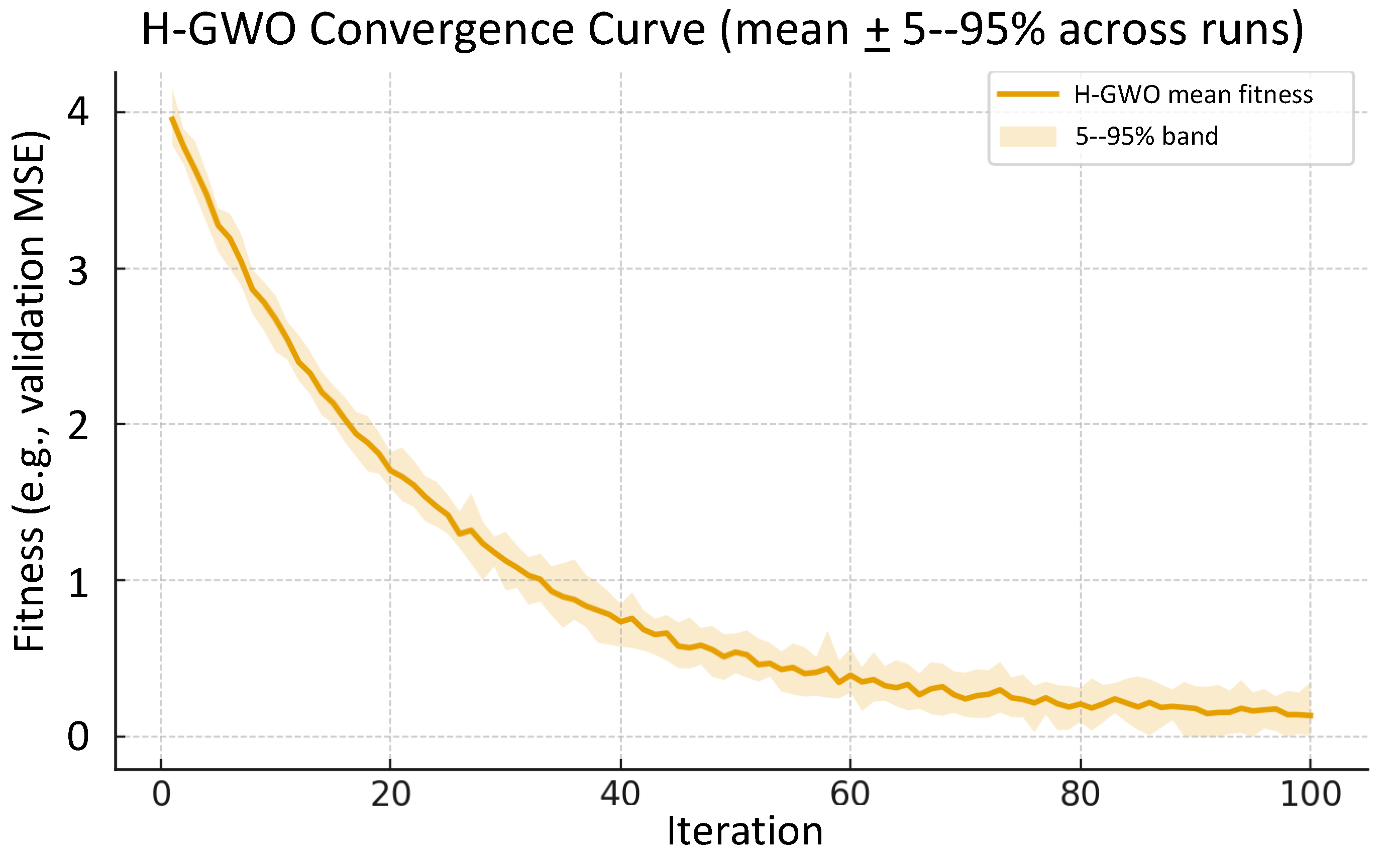
To evaluate the effectiveness of H-GWO in hyperparameter search, the convergence curve of fitness values during the optimization process was plotted, as shown in Figure 6. It can be observed that the fitness value decreases rapidly in the early stage, suggesting that the algorithm is able to quickly locate promising solutions in the search space. As the number of iterations increases, the curve gradually stabilizes, indicating that H-GWO has essentially converged and identified an optimal set of hyperparameters at the global level. This result demonstrates the strong global search ability and stability of the proposed method in the optimization process.

H-GWO optimizes the convolution kernel size of the TCN layers, the number of BiLSTM neurons, the dropout rate, the learning rate, and the batch size for the prediction model. For the output data dimension of the TCN layer and the activation function of the BiLSTM layer, manual comparison and selection are carried out. After optimization, the optimal parameter combination of the TCN-BiLSTM-MHA model is shown in

Table 1. Parameters of TCN-BiLSTM-MHA model optimized by H-GWO.

Parameter Name	Search Domain	Optimal Value of Objective Function
Tcn_kernel_size	[2–10]	5
tcn_out_channels	[16, 32, 64, 128, 256]	32, 64, 128, 128
BILSTM hidden_size	[16–256]	64
BiLSTM activation function	[RELU, sigmoid, tanh]	RELU
Dropout_rate	[0–0.5]	0.3
learning_rate	[0.001–0.01]	0.005
Batch_size	[16–256]	64

.

4. Experimental Verification and Discussion

4.1. Data Preprocessing

4.1.1. Dataset

The dataset used in this paper is an open-source dataset from the LEA Department at Paderborn University [36], and it contains more than 180 h of PMSM data, with a sampling frequency of 2 Hz. It includes 13 features, such as $d/q$-axis current and voltage components, coolant temperature, stator and rotor temperatures, etc. The data collection process adopts a “speed–torque” plane random walk method to accurately simulate real driving scenarios.

To prevent the model from being biased towards high-value features due to large discrepancies in feature values, and considering that the TCN and BiLSTM are sensitive to feature scales, this paper performs normalization processing on the data, as shown in Equation (21).

$$x^{\prime }=a+{\displaystyle \frac{(x-min(x\left)\right)\times (b-a)}{max\left(x\right)-min\left(x\right)}}$$

(21)

where a and b are the lower and upper bounds of the target range.

4.1.2. Correlation Analysis

To reduce the computational cost, improve the model prediction speed, and mitigate the risk of overfitting, we conducted a feature importance analysis based on the original data. First, the Pearson correlation coefficient was calculated to evaluate linear correlations; second, mutual information (MI) was used to capture nonlinear dependencies.

Figure 7 presents the results of the input feature correlation analysis. The results show that stator temperature-related variables (stator_tooth, stator_winding, stator_yoke) are highly linearly correlated with rotor temperature (correlation coefficient > 0.75, MI > 3.4) and serve as the primary predictors. For u_q, u_d, and torque, the Pearson correlation is weak, but MI indicates the presence of nonlinear dependencies with the target variable, so these features were still retained. In contrast, the MI values of coolant temperature and profile_id are significantly lower (<1), providing essentially no valid information, so they were excluded. Finally, we selected {stator_tooth, stator_winding, stator_yoke, u_q, u_d, torque} as the main inputs for the model.

Based on the complete operating cycle of the motor, the dataset is divided into a training set, validation set, and test set at a ratio of 6:2:2, with the aim of avoiding splitting continuous data under the same operating condition into different subsets.

4.2. Experimental Setup and Evaluation Metrics

All models in this experiment were implemented using the PyTorch 2.1 framework, with the operating environment being Windows 10, an Intel Core i7-9750H CPU (2.6 GHz, 16 G memory) (Intel Corporation, Santa Clara, CA, USA), an NVIDIA GeForce GTX 2060 GPU (6 GB video memory) (Nvidia Corporation, Santa Clara, CA, USA), and CUDA 12.6.

In the experiment, a sliding window was constructed based on the continuous time series, with a step size of 1 and a window length of 64. For the 7 input features, continuous sampled data (including historical and current moments) were used to form the input sequence, and the rotor temperature was derived through changes in input features in the historical time period. The model continuously predicts the rotor temperature at a single time step, and prediction results are not fed back as model inputs, thus avoiding the accumulation of prediction errors. The Adam optimizer is used, and the learning rate gradient is reduced to achieve gradual convergence, with the MSE as the loss function.

The experiment selects MAE, RMSE, and coefficient of determination ($R^2$) as evaluation metrics. The calculations of each evaluation metric are shown in Equations (22)–(24).

$$\mathrm{MAE}={\displaystyle \frac{1}{n}}\sum _{i=1}^n\left|{\widehat{y}}_i-y_i\right|$$

(22)

$$\mathrm{RMSE}=\sqrt{{\displaystyle \frac{1}{n}}\sum _{i=1}^n{\left({\widehat{y}}_i-y_i\right)}^2}$$

(23)

$$R^2=1-{\displaystyle \frac{{\sum }_{i=1}^n{\left({\widehat{y}}_i-y_i\right)}^2}{{\sum }_{i=1}^n{\left({\overline{y}}_i-y_i\right)}^2}}$$

(24)

4.3. Model Performance Experiment

4.3.1. Ablation Experiment

Based on the model structure proposed in this paper, three variant models are constructed, namely, TCN, TCN-BiLSTM, and TCN-BiLSTM-MHA, to systematically evaluate the role of each module in the overall model performance. Based on repeated predictions on the test set, Figure 8 shows the convergence process of the loss function derived from the mean squared error during training, and

Table 2. Model performance indicators.

Model	MAE	RMSE	R2
TCN	0.6126	0.7759	0.9482
TCN-BiLSTM	0.4370	0.5706	0.9611
TCN-BiLSTM-MHA	0.4019	0.5314	0.9785
H-GWO-TCN-BiLSTM-MHA	0.3807	0.4839	0.9988

presents a comparison of performance metrics among the models on the test set. It can be seen that the H-GWO-TCN-BiLSTM-MHA model has the fastest convergence speed, the lowest loss value, and the optimal prediction indicators. A comparison with TCN-BiLSTM-MHA shows that hyperparameter optimization via H-GWO addresses the inefficiency and instability of manual parameter tuning. Meanwhile, the convergence curves show that H-GWO-TCN-BiLSTM-MHA and TCN-BiLSTM-MHA converge more quickly and stably than the other two models, and the test results are better, indicating that the MHA module can significantly enhance the model’s ability to extract important features and key trends and can effectively suppress irrelevant interference information, playing an important role in the model’s prediction results. The comparison between the TCN and TCN-BiLSTM proves that the combined structure of the two can capture both local temporal features and long-distance dependent information, thereby improving the accuracy and robustness of time-series modeling, and has more advantages than a single model.

4.3.2. Comparison of Prediction Performance of Different Models

To verify the effectiveness of the proposed model, three comparative models (DFNN, BiLSTM-Attention, and CNN-BiLSTM-Attention) are proposed based on existing research on motor temperature prediction [18,19,20]. To ensure the validity of the comparative experiments, all models were trained under the same experimental environment and training set conditions.

Based on repeated predictions on the test set,

Table 3. Comparison of evaluation metrics of different models.

Model	MAE	RMSE	R2
DFNN	0.6783	0.8229	0.9257
BiLSTM-Attention	0.4711	0.6206	0.9492
CNN-BiLSTM-Attention	0.4330	0.6017	0.9694
H-GWO-TCN-BiLSTM-MHA	0.3821	0.4857	0.9985

presents the prediction metrics of each model on the test set. It can be seen that the H-GWO-TCN-BiLSTM-MHA model proposed in this paper exhibits high prediction accuracy, with MAE and RMSE being 0.3821 and 0.4857, respectively. Compared with the CNN-BiLSTM-Attention (an efficient prediction model widely used in recent years), the MAE and RMSE are reduced by approximately 11.8% and 19.3%, respectively, and it also achieves an $R^2$ of 0.9985. Four randomly selected operating conditions in the test set are shown in Figure 9. The statistics of the absolute prediction errors of the four models on the entire test set are shown in Figure 10, and Figure 11 displays the comparison between the predicted values and the true values of the four models on part of the test set. The maximum absolute prediction error of the H-GWO-TCN-BiLSTM-MHA model on the complete test set does not exceed 1.7 °C, with an average absolute error of 0.3821 °C.

To further enhance the reliability of the model in safety-critical scenarios, this study employs the MC-Dropout method during the prediction phase to model predictive uncertainty. By keeping Dropout active at inference and performing multiple forward passes, the predictive distribution is obtained. The results show that the true temperature has a mean of 64.998 °C and a variance of 18.762, while the predicted temperature has a mean of 64.601 °C and a variance of 18.525. To evaluate the effectiveness of the prediction intervals, the Prediction Interval Coverage Probability (PICP) is adopted as the calibration metric. At the 95% confidence level, the model achieves a PICP of 0.975, which is higher than the nominal coverage of 0.95. This indicates that the prediction intervals generated by MC-Dropout are relatively conservative but can effectively cover the true rotor temperature, thereby ensuring higher reliability in safety-critical thermal monitoring applications.

In addition, Figure 12 shows a residual analysis. The Q-Q plot indicates that the residuals approximately follow a normal distribution. The blue circles represent the quantiles of the residuals from our model, and the red line is the reference line for the theoretical normal quantiles. The residual histogram shows that the residuals are centered near zero, and their frequency rapidly decreases as the deviation from zero increases.

In general, H-GWO-TCN-BiLSTM-MHA shows advantages in multiple evaluation metrics and has advantages in the task of predicting the rotor temperature of permanent magnet synchronous motors.

5. Conclusions

To address the challenge of rotor temperature prediction in permanent magnet synchronous motors (PMSMs), this paper proposes a hybrid deep learning model integrating a TCN, BiLSTM, and MHA and introduces an improved Hybrid Grey Wolf Optimization algorithm to optimize the model parameters. Experiments are conducted using a public motor dataset. Data standardization and feature analysis are performed first, followed by constructing the prediction model and evaluating its performance. The experimental results show that the proposed H-GWO-TCN-BiLSTM-MHA model achieves excellent prediction accuracy on this dataset, with an MAE of 0.3821 °C and an RMSE of 0.4857 °C. Its overall performance is superior to that of existing comparative models, verifying its effectiveness and robustness in motor rotor temperature modeling and prediction tasks. In future work, the model can be further optimized to be adapted to edge computing or embedded deployment scenarios, and integrated into intelligent motor monitoring systems to achieve efficient and real-time prediction of rotor temperature. In addition, it can be combined with more operating condition data and online learning mechanisms to enhance the model’s generalization ability and stability under complex operating conditions.