Article

Railway Fastener Defect Detection Model Based on Dual Attention and MobileNetv3

School of Mechanical Engineering, Lanzhou Jiaotong University, Lanzhou 730070, China
*
Author to whom correspondence should be addressed.
World Electr. Veh. J. 2025, 16(9), 513; https://doi.org/10.3390/wevj16090513
Submission received: 10 June 2025 / Revised: 15 August 2025 / Accepted: 8 September 2025 / Published: 11 September 2025

Abstract

Defect detection in rail fasteners constitutes a fundamental requirement for ensuring safe and reliable railway operations. Confronted with increasingly demanding inspection requirements of modern rail networks, traditional manual visual inspection methods have proven inadequate. To achieve accurate, efficient, and intelligent detection of rail fasteners, this paper presents an enhanced YOLOv5m-based defect detection model. Firstly, a dual-attention mechanism comprising Squeeze-and-Excitation and Coordinate Attention modules is employed to enhance the model. Secondly, the network architecture is redesigned by adopting MobileNetv3 as the backbone while incorporating structures with Ghost Shuffle Convolution (GSConv) modules and lightweight upsampling operators to reduce computational overhead. Finally, the original CIoU loss function in YOLOv5 is replaced with SIoU to accelerate convergence rate during training. Experimental results on a custom-built rail fastener dataset comprising 6500 images demonstrate that the enhanced model achieves 96.5% mAP and 17.9 FPS, surpassing the baseline by 3.1% and 2.1 FPS, respectively. Compared to existing detection models, this solution exhibits higher accuracy, faster inference, and lower memory consumption, providing critical technical support for edge deployment of rail fastener defect detection systems.

1. Introduction

Railway tracks are typically composed of two parallel steel rails, secured by rail components such as rail braces, fasteners, fishplates, clips, and rail spikes. Due to the immense pressure railway tracks must endure, the rails are manufactured from high-quality steel, commonly referred to as the tracks. Rail fasteners, as critical components that rigidly secure the rails to the sleepers, play a vital role in ensuring railway operational safety. Research in the railway industry indicates that rail fasteners may develop initial defects due to substandard manufacturing processes, and the severity of these defects intensifies with prolonged use [1]. Additionally, prolonged exposure to harsh natural environments or even malicious human interference can lead to loosening or damage of the fasteners. Safety data from the U.S. Federal Railroad Administration reveals that, out of 651 train derailments in 2013, 27 were caused by defects in rail spikes or fasteners [2]. The service condition of fasteners directly impacts railway operational safety, making timely and accurate quantitative detection of fastener damage essential for ensuring the stable operation of railway systems.
Traditional manual inspection methods are labor-intensive and time-consuming, exploring efficient defect detection technologies for rail fasteners has long been a critical task in railway inspection. In the late 20th century, the TVIS system developed by ENSCO in the United States and Germany’s RAILCHECK track inspection system incorporated high-speed image acquisition and processing algorithms to identify missing fasteners, yet they failed to detect more complex defects [3,4]. In the early 21st century, Ref. [5] combined wavelet transforms with principal component analysis (PCA) for image preprocessing and utilized both backpropagation neural networks and radial basis function neural networks as classifiers to analyze fastener images, thereby enhancing rail fastener detection efficiency. However, the directional sensitivity of wavelet transforms and the global dimensionality reduction characteristics of PCA easily lead to the loss of local defect information, and the cascaded feature extraction process significantly increases computational overhead. Ref. [6] proposed a fastener defect detection method based on enhanced edge feature analysis. The approach employed a median filtering technique to extract edge features, followed by an optimized Canny edge detection algorithm to improve edge localization accuracy. Subsequently, the extracted features were matched against predefined defect templates to enable real-time fastener inspection. Similarly, Refs. [7,8] introduced a multi-task learning (MTL) framework for fastener defect detection, integrating multiple detectors to enhance recognition performance. The proposed method utilized Histogram of Oriented Gradients (HOG) descriptors to extract discriminative fastener features from input images. Subsequently, a Support Vector Machine (SVM) classifier was employed to categorize fastener conditions, including damaged and missing defects. This approach demonstrated improved detection robustness by leveraging the complementary strengths of feature-based and machine learning techniques. However, these methods exhibit significant limitations as follows: heavy reliance on handcrafted features results in insufficient robustness against noise, illumination variations, and structural deformations; predefined templates or fixed feature extractors fail to adequately cover complex and variable defect patterns such as corrosion, fractures, and occlusions, leading to weak generalization capability; and the multi-stage processing pipeline incurs substantial computational overhead, making it difficult to meet the real-time inspection demands of high-speed railways.
Compared to traditional methods combining image processing and statistical learning, deep learning leverages the powerful feature representation capability of convolutional neural networks (CNNs) to automatically extract image features based on inherent visual characteristics, enabling advanced object recognition and classification. This end-to-end learning paradigm overcomes the limitations of manual feature engineering, demonstrating superior robustness and accuracy when handling complex and variable industrial imaging data. Its precision and efficiency in detecting diverse complex defects significantly outperform conventional approaches. Deep learning-based anomaly detection algorithms are typically categorized into two types: two-stage detection algorithms and one-stage detection algorithms.
Two-stage detection algorithms first generate candidate regions through a Region Proposal Network (RPN), then classify and regress targets within these regions to determine their precise locations and categories. Representative algorithms include Faster R-CNN and Mask R-CNN. Ref. [9] employed the Faster R-CNN model to improve detection efficiency for railway track fasteners. Ref. [10] simplified and optimized Faster R-CNN by adopting K-means clustering to automatically identify anchor positions, thereby enhancing detection performance for imbalanced fasteners. Although these methods achieve improved detection accuracy, they suffer from large parameter volumes and still require speed optimization. One-stage detection models such as YOLO and SSD directly localize and classify target objects without predefined anchor boxes [11,12], offering higher speed and accuracy for detecting small targets like rail fastener defects. Ref. [13] proposed a cascaded three-stage deep neural network based on YOLO for fastener defect localization and category recognition, achieving high detection rates. Ref. [14] developed the TLMDDNet model based on YOLOv3 for multi-target detection in railway scenarios, incorporating multi-level scaling and feature concatenation. Ref. [14] introduced a lightweight detection model named YOLOv5_SS, which utilizes the Soft-NMS algorithm to improve detection of densely overlapping objects. While these studies demonstrate significant improvements in detection accuracy and resource efficiency, several challenges persist as follows: false positives, missed detections, and redundant detections of multi-scale and occluded targets. Additionally, issues including coarse feature extraction and insufficient localization accuracy in one-stage networks remain inadequately resolved.
To address these limitations, this study enhances the native YOLOv5m by introducing a dual attention mechanism that calculates spatial and channel weights to improve feature extraction and fusion capabilities; replacing the original CSPDarkNet backbone with the lightweight MobileNetv3 convolutional network while adopting lightweight upsampling operators; and further integrating a GSConv-incorporated Slim-Neck structure into the model’s Neck section and implementing SIoU as the bounding box regression loss function, collectively achieving model lightweighting and detection accuracy improvement. The enhanced model was subsequently trained on a rail fastener dataset, with the final trained weights used to validate whether the optimized model satisfies the high-accuracy and real-time requirements for fastener defect detection.

2. YOLOv5 Improvement

2.1. Attentional Mechanisms

YOLO (You Only Look Once) is a deep neural network-based algorithm for object recognition and localization, proposed by Redmon et al. [15] in 2015, and is well-suited for lightweight, efficient single-stage object detection tasks. The YOLO series algorithms have now evolved to YOLOv10, with YOLOv5 being the most mature and widely used generation, serving as a typical representative of the YOLO series. Based on this, this study selects YOLOv5 as the baseline model for algorithm improvement. Compared to its predecessor YOLOv4, YOLOv5 introduces Mosaic data augmentation, adaptive anchor box computation, and adaptive image scaling at the input stage. It incorporates a Focus structure and a Cross Stage Partial (CSP) architecture into the convolutional network. A feature pyramid is added between the Backbone and the final Head output layer to enhance semantic information propagation and feature extraction. The YOLOv5 model architecture primarily consists of four components: the Input layer, Backbone network, Neck network, and Head output layer. Taking a rail fastener image as an example, the image is compressed into a 3D feature map as input. Through convolutional operations in the Backbone, the fastener image is divided into an S × S grid, where each grid cell predicts N bounding boxes along with their confidence scores and class probabilities. During detection, the entire image is fed into the model. In the Backbone, Conv modules perform convolutional computations and batch normalization. The input is then split into two branches via the C3 module’s CSP structure for parallel convolutional processing. Finally, Spatial Pyramid Pooling (SPP) is applied to expand the network’s receptive field, generating multi-dimensional feature maps. In the Neck section, feature maps are fused through Concat layers, and image resolution is enhanced via UpSample layers for upsampling [16]. The Head layer subsequently processes these fused features through Conv2d operations, outputting feature maps of varying scales along with the positions, categories, and confidence levels of all detected fasteners.

2.2. Dual Attention Mechanism

The core idea of the attention mechanism is to dynamically assign varying weights to input data, enabling the model to focus on the most relevant information, thereby enhancing its performance and generalization capability.
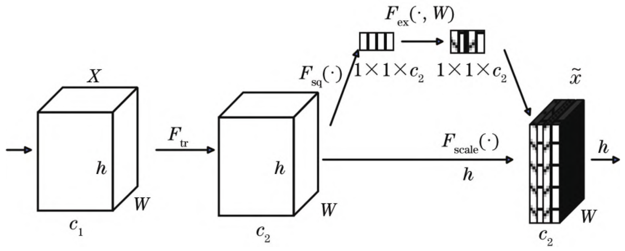
Many convolutional networks including MobileNetv3 have adopted the Squeeze-and-Excitation (SE) attention mechanism [17]. As shown in Figure 1, the SE attention mechanism primarily undergoes Squeeze, Excitation, and Scale operations (labeled as F s q , F e x , and F s c a l e in the figure, respectively). During operation, first, feature x from h × W × c 1 undergoes a convolution F t r to form feature h × W × c 1 ; then the Squeeze operation compresses each channel’s 2D feature h × W into a single real number through global average pooling, compressing the feature map from h , W , c 2 along the W dimension to 1 , 1 , c 2 , obtaining channel-level global features; during the Excitation operation, weight values are assigned to each feature channel (different patterns in the figure represent different weights) to establish inter-channel relationships, where the number of output weight values equals the number of input feature map channels; and during the Scale operation, dimensionality is restored by weighting the previously obtained normalized weights onto each channel’s features, ultimately forming feature x ˜ of h , W , c 2 .
Although the SE (Squeeze-and-Excitation) attention mechanism helps the model focus on the most informative channel features while suppressing less important ones, it solely considers inter-channel relationships while neglecting positional information. When multiple fastener samples appear in an image, this limitation can lead to inaccurate bounding box predictions. To address this issue while retaining the SE mechanism, we incorporate an efficient attention mechanism—Coordinate Attention (CA) [18]—to capture spatial positional information from images, thereby forming a dual-attention mechanism.
Figure 1. Working principle of SE attention mechanism. Reprinted with permission from Ref. [19]. Copyright 2025 Computer Engineering Editorial Office.
Wevj 16 00513 g001
Figure 2 illustrates the schematic diagram of the CA (Coordinate Attention) mechanism. For the i-th channel of a feature map with dimensions H × W × i , the CA mechanism performs pooling along both the horizontal (X) and vertical (Y) directions for the element at coordinate (a,b), generating feature maps of dimensions H × i × 1 and W × 1 × i , respectively. At height h and width w positions, the following equations are satisfied as follows:
z i h h = 1 W 0 a < W x i h , a
z i h w = 1 H 0 a < H x i b , w
In the equations, z i h h and z i h w represent the pooled feature maps along the height and width directions, respectively; x i h , a denotes the global average pooling output at coordinate a , b along the height dimension; and x i b , w corresponds to the global average pooling output at coordinate a , b along the width dimension.
Using Equation (1), features are aggregated separately along the two spatial directions to obtain a pair of attention-aware feature maps. By applying Equations (1) and (2), features are further aggregated along both spatial directions, yielding a pair of enhanced attention-aware feature maps. The resulting H × i × 1 and W × 1 × i feature maps are then concatenated and processed through a 1 × 1 convolutional module F 1 × 1 for dimensionality reduction, compressing the channels to i / r (r is the reduction factor for the feature map’s dimensionality (or channel count), serving to reduce computational cost, memory usage, and prevent overfitting). Subsequently, batch normalization and a nonlinear activation module (BatchNorm + Nonlinear in Figure 2), followed by a Sigmoid activation function (σ), are applied to generate the final attention feature map f, expressed as follows:
f = σ F 1 × 1 z ( h ) , z ( W )
Two additional 1 × 1 convolutional transformations, Fn and Fw (representing the two spatial directions), process the pooled feature maps fh (horizontal) and fw (vertical), respectively. These are then activated via the sigmoid function σ to generate directional attention weights gh and gw. These weights are subsequently integrated to produce the final output yᵢ of the Coordinate Attention (CA) mechanism.
g h = σ F h f h
g w = σ F w f w
y i a , b = x i a , b × g h , i a × g w , i b
gh,i and gw,i represent the attention weights of the i channel along the horizontal and vertical directions, respectively.
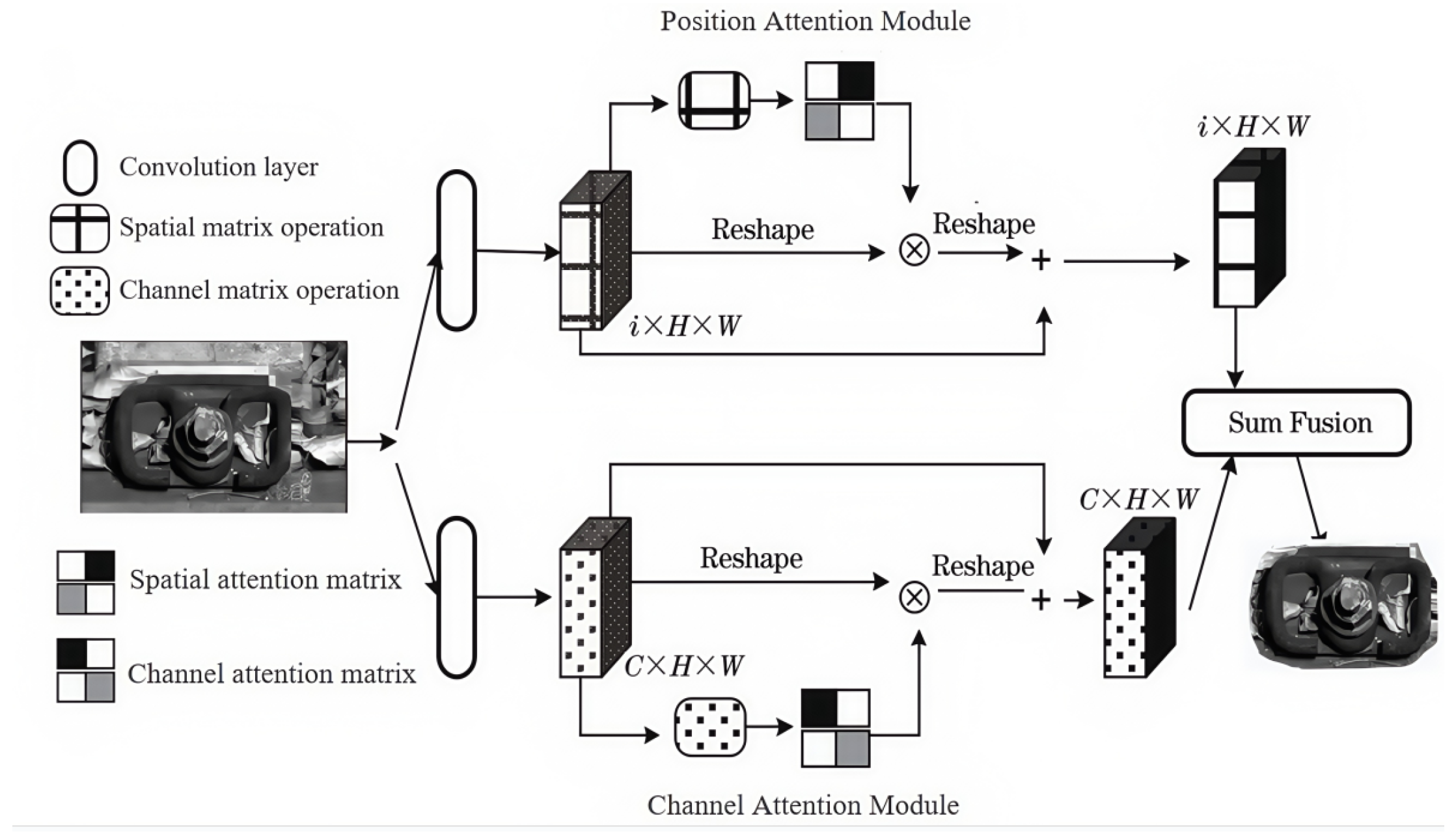
As shown in Figure 3, the SE module serves as the channel attention mechanism while the CA module functions as the positional attention mechanism. After undergoing reshape and convolutional operations, their outputs are combined through matrix summation. This dual-attention integration enhances the model’s capability for target localization and recognition, while the reduced dimensionality contributes to lower computational overhead, ultimately leading to a more lightweight model architecture. Compared to the channel recalibration of traditional SENet, the coordinate-decomposed attention of CA-Net, and the serial local perception of CBAM, the dual-attention mechanism structure—by paralleling the position attention module with the channel attention module—effectively captures long-range contextual information, providing superior support for detection tasks reliant on global understanding.

2.3. Application of Lightweight Upsampling Operator CARAFE

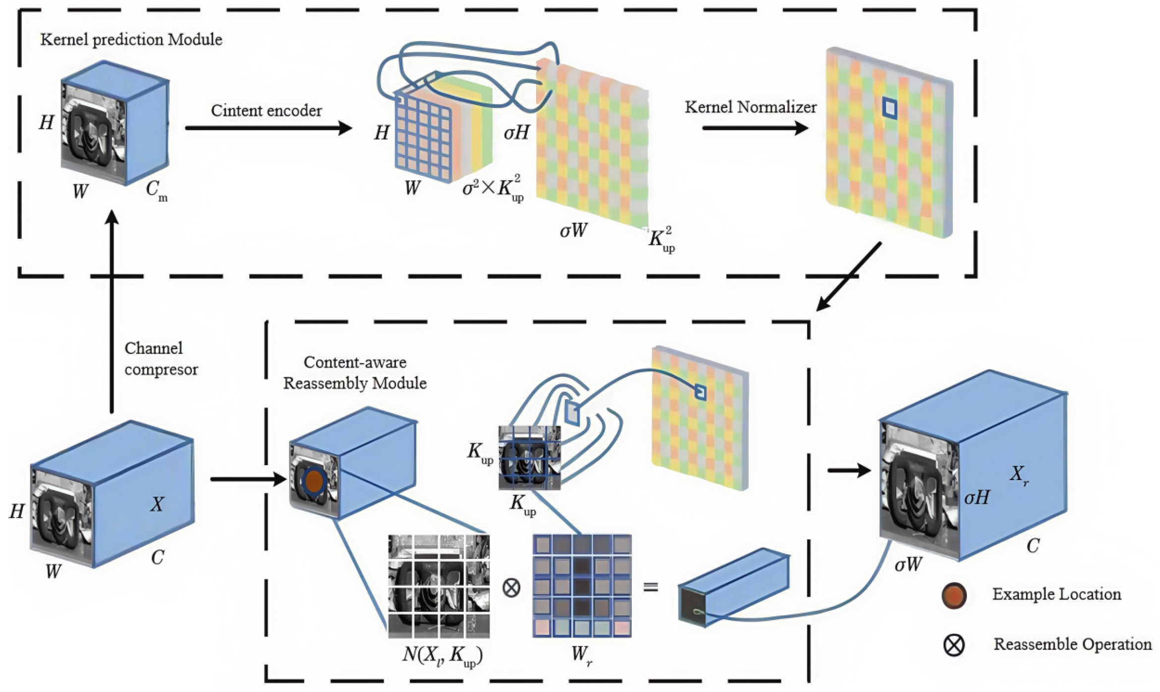
The original upsampling operator in YOLOv5m employs the nearest-neighbor interpolation method, which determines the upsampling kernel solely based on the spatial positions of pixels and does not utilize the semantic information from feature maps. Consequently, the receptive field is typically very small (only 1 × 1). To achieve both a larger receptive field and lightweight design without introducing excessive parameters or computational overhead, this paper proposes replacing YOLOv5m’s upsampling operator with the lightweight and versatile CARAFE upsampling operator. The overall framework of CARAFE is illustrated in Figure 4.
In Figure 4, let us assume we have feature map X with a given size C × H × W and an upsampling rate σ ( σ = 2 ). K up represents the size of the upsampling kernel, C m represents the number of channels in the compressed feature map. Within the content-aware feature reorganization module, let N X l , k represent a k × k -sized local region of feature map X centered at position l . Here, W l denotes the position-specific kernel predicted by the kernel prediction module for each location l based on X l . We first convolve N X l , k with W l while applying kernel regularization. The feature map is then unfolded along the channel dimension to generate a predicted feature map of shape σ W × σ H × K up 2 , where each feature value corresponds to a distinct upsampling kernel. For each upsampling kernel, we first project it back onto the input feature map to retrieve the corresponding feature values. These values are then multiplied via dot product with the kernel weights, ultimately generating the upsampled output feature map.
In small-sized images, small objects or fine structures face a higher risk of information loss during multiple downsampling steps. Standard upsampling methods struggle to effectively recover these minute yet crucial details. The CARAFE operator discards the fixed sampling patterns of traditional upsampling methods (such as bilinear interpolation and transposed convolution). Instead, it dynamically predicts an optimal small reassembly kernel for each target location based on the local content surrounding it in the input feature map. This adaptability enables it to intelligently handle different regions as follows: reinforcing details in areas with complex textures or sharp edges, while applying smooth transitions in flat regions. Consequently, it significantly reduces common post-upsampling issues like blurring and checkerboard artifacts. Simultaneously, by leveraging information from a larger receptive field during reassembly, CARAFE can more effectively recover details lost during downsampling (which is particularly critical for small-sized images with higher information density). Moreover, its lightweight design ensures computational efficiency.

2.4. Lightweight Integration of MobileNetV3 Backbone with GSSN Architecture

In the network architecture construction of our model, this paper employs the lightweight MobileNetV3 as the backbone network. Initially proposed by Google in 2017, the MobileNet series of convolutional neural networks demonstrates that MobileNetV3 [20,21] reduces parameters by approximately 20% while achieving 6.6% higher accuracy compared to MobileNetV2. MobileNetV3 utilizes Depthwise Separable Convolution (DSC) [22] as its fundamental building block. The DSC comprises two components: depthwise convolution and pointwise convolution. During depthwise convolution, each channel of the feature map is processed by an independent convolutional kernel, where the number of kernels equals the number of channels. The mathematical expression is as follows:
F α , β , i = a = 1 W b = 1 H C a , b , i F α + a , β + b , i
The expression is defined as where F α , β , i is the output feature map after depthwise convolution; C a , b , i represents the convolutional kernel at coordinate a , b in the i-th channel; F α + a , β + b , i denotes the output feature map obtained by convolving along both width and height dimensions using the i-th convolutional kernel followed by applying the weight element at coordinate α , β .
During pointwise convolution, the kernel size is first set to 1 × 1 , where depthwise convolution extracts features per channel before establishing inter-channel correlations through pointwise operations. The computational cost D of DSC combining depthwise and pointwise convolutions is expressed as follows:
D = D C D C M D F D F + M N D F D F
The expression is defined as where D F and N denote the side length and channel count of input feature map F , respectively, D C represents the side length of the depthwise convolution kernel, and M corresponds to the channel number of pointwise convolution.
Compared with standard convolution, the computational cost reduction in DSC is given by the following:
D C D C M D F D F + M N D F D F D C D C M N D F D F = 1 N + 1 D C 2
When employing an n × n convolution kernel (where DC takes any positive integer value n ), the computational cost of DSC is only 1 / n 2 of standard convolution [23], achieving network lightweighting.
Although DSC reduces the overall model size and computational load, its decomposition into depthwise and pointwise convolution operations compromises feature extraction and fusion capabilities compared to standard convolution (SC).
To enable DSC’s output to closely approximate SC while preserving feature extraction capability, we introduce a novel module—GSConv [24]—into the Neck section of YOLOv5m.
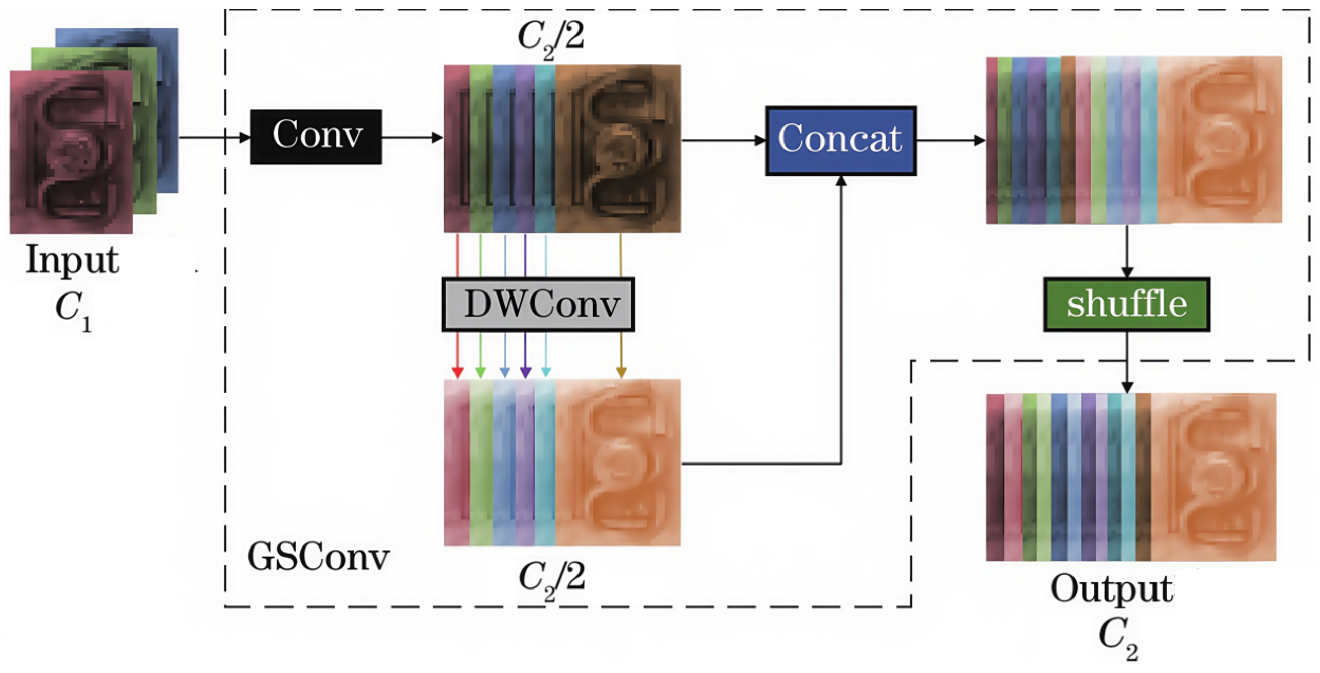
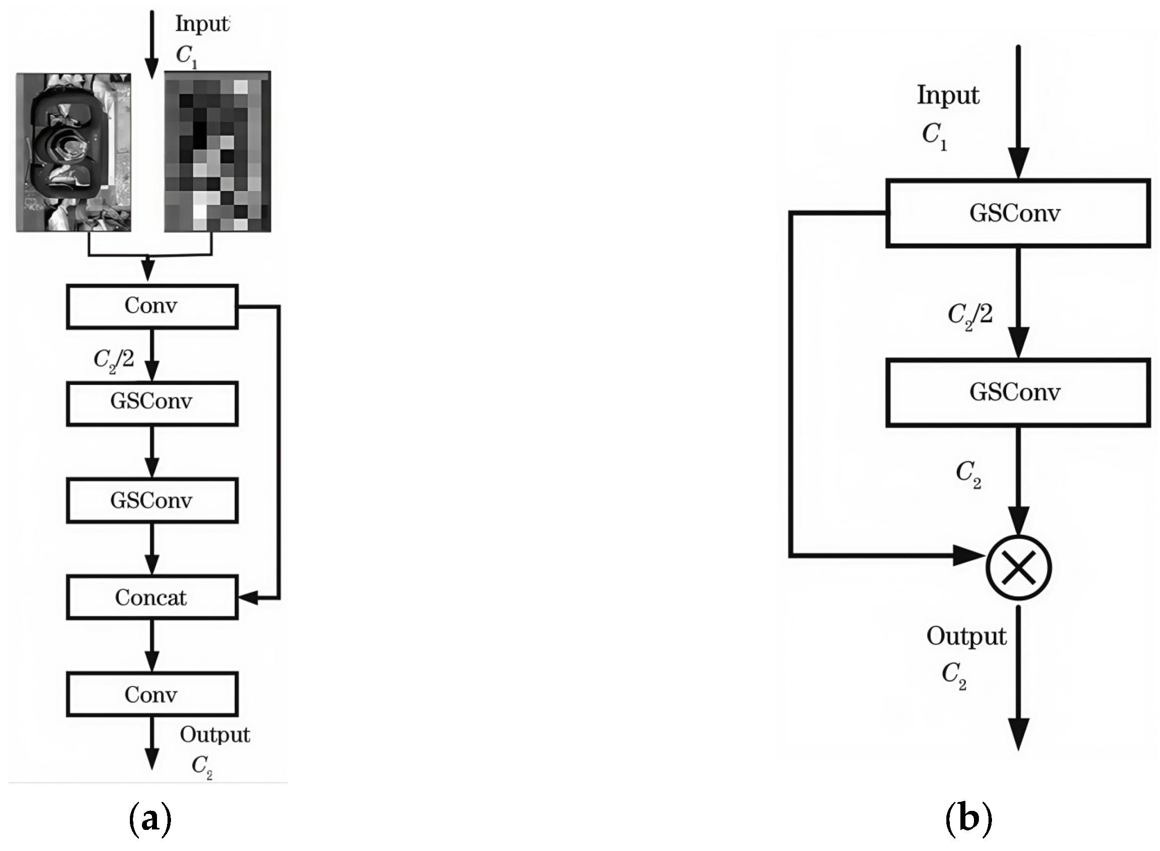
As illustrated in Figure 5, the input image with C 1 channels undergoes depthwise separable operation (DWConv), followed by channel-wise concatenation of pre- and post-separation features. Subsequent dense convolution operation employs channel shuffle to permeate SC-generated information throughout all components of DSC-generated features—specifically maintaining C 2 / 2 channels before and after DWConv, respectively. The final output yields C 2 channels with 30–40% reduced computational cost compared to SC [25], while fulfilling lightweight requirements.
Figure 6 illustrates the architecture of the cross-stage VoV-GSCSP network based on GSConv and CSP, along with its bottleneck unit design. By first concatenating two feature maps with width w and height h , respectively, followed by convolution, the module enhances information fusion and interpretability.
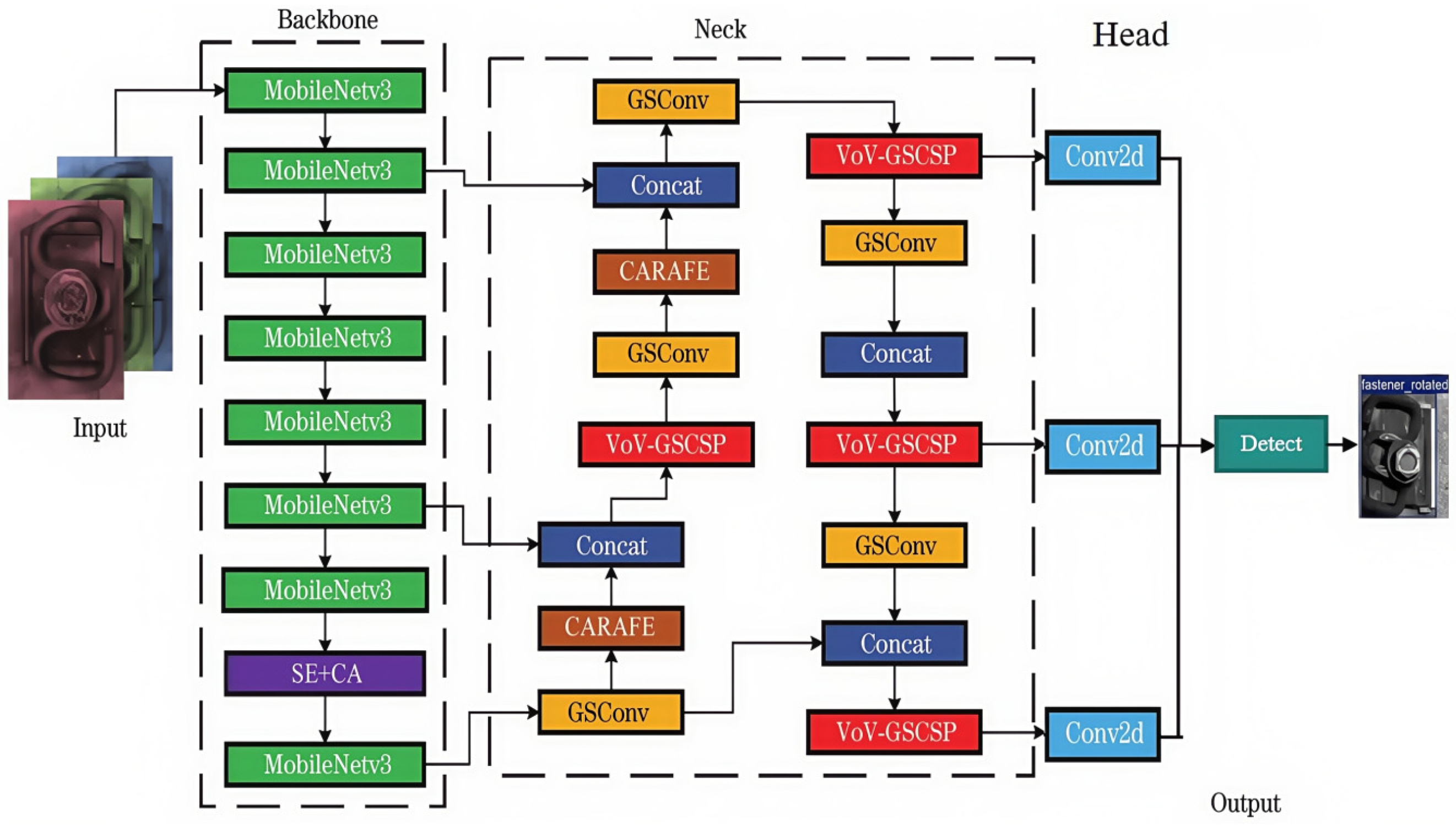
The YOLOv5m network architecture undergoes strategic modifications in its Neck section by replacing standard Conv modules with GSConv coupled with concatenation operations, while simultaneously substituting C3 modules with VoV-GSCSP modules to construct the Slim-Neck structure. This Slim-Neck configuration achieves parameter reduction through decreased channel numbers in intermediate layers, with the GSConv-incorporated variant being formally designated as the GSSN (GS Slim-Neck) structure. The GSSN architecture maintains equivalent training and detection accuracy while delivering substantial reductions in both model complexity and storage resource consumption.
The improved lightweight YOLOv5 framework, as shown in Figure 7, is achieved through the integration of two key modules—a dual attention mechanism and a lightweight upsampling operator—along with lightweight replacement of the backbone network and structural innovations in the Neck section.

3. Dataset Preparation and Experimental Setup

3.1. Dataset Preparation and Environment Setup

The dataset in this study was difficult to collect due to environmental factors and railway regulations. Through field investigations at a test line of a Hebei-based company, we captured and organized 6500 rail fastener images covering four working conditions: normal (labeled as normal), missing elastic rail clip (missing), fractured elastic rail clip (fracture), and displaced elastic rail clip (deflection), with each image having a resolution of 150 × 225 pixels. A total 80% of the dataset was used as the training set, with the image quantities for each condition shown in Table 1.
The experimental model in this study was trained on an NVIDIA RTX 3080 10 GB GPU (29.77 TFLOPS single-precision), with Python 3.8, Ubuntu 18.04 OS, PyTorch 1.9.0 framework and CUDA 11.1. Detection and evaluation were performed on an edge computing platform—an NVIDIA Jetson TX2 equipped with a quad-core ARM Cortex-A57 MPCore processor, 256-core NVIDIA Pascal architecture GPU, and 8GB 128-bit LPDDR4 memory.

3.2. Training Parameters and Evaluation Metrics

To ensure a clear comparison with the original YOLOv5m, the hyperparameters in this study were kept essentially identical to the default settings of YOLOv5m, as detailed in Table 2.
The Mosaic data augmentation technique randomly selects a set of images during each training epoch, applies random scaling, cropping, brightness adjustment, and other transformations, then stitches them together to create new training samples—significantly enhancing the model’s robustness.
To evaluate the lightweight performance of the improved model, we employ two key speed metrics: average single-image processing time and frames per second (FPS). For accuracy assessment, we adopt standard object detection metrics including precision (P), recall (R), and mean average precision ( A m A P ) [26]. Precision reflects the proportion of true positive samples among all predicted positive cases, representing the probability of correct positive predictions, which can be expressed as follows:
P = N TP N TP + N FP
where N TP represents the number of true positives; N FP denotes the number of false positives.
Recall represents the proportion of correctly predicted positive samples among all actual positives, reflecting the model’s ability to avoid missed detections, which can be expressed as follows:
R = N TP N TP + N FN
The mean average precision can be expressed as follows:
A mAP = i = 1 n A i n
where n denotes the number of categories; A i represents the average precision for class i . The experiment requires predefining the Intersection over Union (IoU) threshold between predicted and ground-truth bounding boxes. The mean average precision in this study is calculated as the average of per-class AP values at an IoU threshold of 0.5.

3.3. Coordinate Loss Function Configuration

To address the overlapping occlusion between rail fastener nuts and elastic clips, as well as distance, aspect ratio, and angular deviations, this study employs SIoU [27] as the coordinate loss function. By imposing precise constraints on the predicted bounding boxes along either the x-axis or y-axis, SIoU enhances convergence speed while reducing computational overhead, thereby achieving model lightweighting. The SIoU loss consists of four components: angle cost ( L angle ), distance cost ( L dis ), shape cost ( L shape ), and IoU loss.
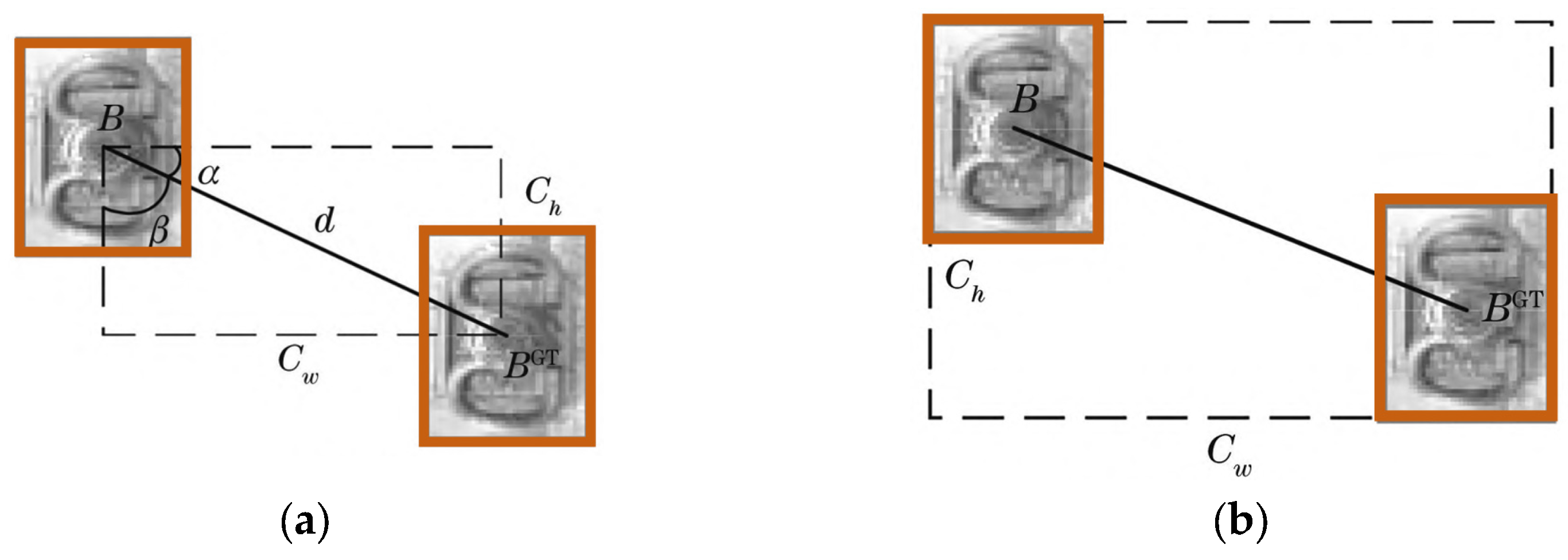
The angle cost computation process is illustrated in Figure 8a. Starting from the predicted bounding box’s center point B b c x , b c y (hypothetically corresponding to the nut center), we constrain either its horizontal or vertical axis relative to the ground truth box’s center B GT b c x GT , b c y GT to reduce anchor box degrees of freedom. Here, d and C h represent the distance and height difference between the ground truth and predicted box centers, respectively. The angle cost is calculated as follows:
L angle = 1 2 sin 2 arcsin C h d π 4 = 1 2 sin 2 α π 4
The distance cost L dis computation process is demonstrated in Figure 8b, where the diagonal distance of the minimum enclosing rectangle between predicted and ground truth boxes is calculated as follows:
L dis = 2 e γ ρ x e γ ρ y ρ x = b c x gt b c x C w 2 ρ y = b c y gt b c y C h 2 γ = 2 L angle
where C w denotes the width of the minimum enclosing rectangle.
L shape = 1 e w w θ + 1 e w h θ w w = w w gt max w , w gt w h = h h gt max h , h gt
w gt and h gt denote the width and height of the ground truth box, respectively, while θ controls the weight of shape loss to prevent excessive focus on fastener defect shapes from restricting the predicted box’s movement during detection.
The SIoU loss function is formulated as follows:
L SIoU = 1 R IoU + L dis + L shape 2
where R IoU represents the correlation coefficient between the ground-truth defect location and the predicted position.

4. Experimental Results Analysis

4.1. Model Training Results

The native YOLOv5m was configured according to the improvement scheme proposed in this paper with hyperparameters set, as shown in Table 2, to initiate model training. As illustrated in Figure 9a–c, the YOLOv5m loss function consists of coordinate loss (box_loss), confidence loss (obj_loss), and classification loss (cls_loss). The box_loss measures the model’s predictive capability for localization errors between predicted and ground-truth bounding boxes, the obj_loss evaluates the model’s target detection ability, while the cls_loss assesses the model’s target classification performance. All three loss components gradually converge as training iterations increase. Figure 9d demonstrates that the A m A P value increases proportionally with the number of iterations, proving that the average prediction accuracy for various defects in the dataset progressively improves and the model’s predictive capability enhances.
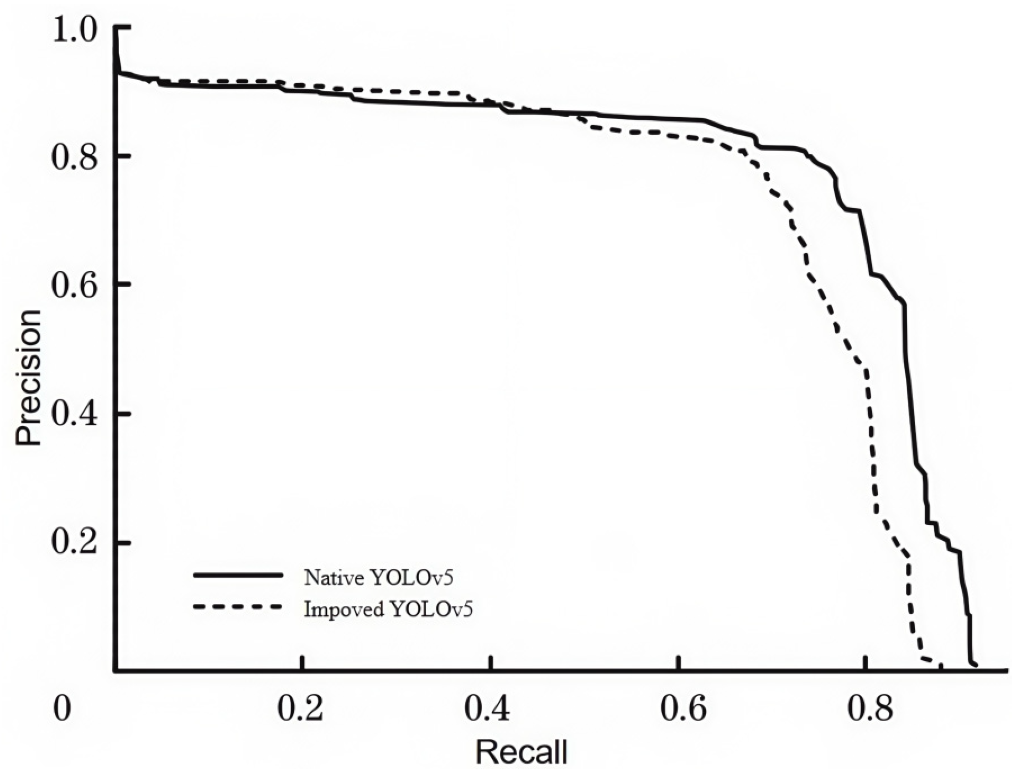
Figure 10 presents the Precision-Recall curves of the model before and after improvement. Compared to the baseline model, the enhanced model exhibits a slower decline in average precision across defect categories as recall increases (corresponding to progressively fewer undetected samples). Its curve encloses a larger area with the coordinate axes, resulting in enhanced recognition performance.

4.2. Comparative Experiments on Improvement Points

To further validate the effectiveness of the proposed improvements on the rail fastener dataset, we conducted comparative experiments by progressively integrating three comparable enhancement components—different backbone networks, attention mechanisms, and loss functions—into the native YOLOv5m model.
As shown in Table 3, comparative experiments were conducted between the original CSPDarkNet backbone network and other lightweight networks. The results demonstrate that ShuffleNetv2 requires less GPU memory than the original backbone but with reduced accuracy; MobileNetv2 shows slightly improved accuracy metrics compared to ShuffleNetv2 yet demands more memory and computational resources; and MobileNetv3 achieves higher accuracy than both alternatives while maintaining intermediate memory usage. Therefore, after comprehensive consideration of both accuracy metrics and memory consumption, the lightweight backbone network adopted in this study demonstrates superior overall performance.
As shown in Table 4, comparative experiments were conducted by incorporating different attention mechanisms into the MobileNetv3 backbone network. The results indicate that (1) When using CBAM, the model achieves 3.0%, 2.1%, and 2.8% higher P, R, and A m A P , respectively, compared to the SE attention mechanism, albeit with greater GPU memory consumption; and (2) The dual attention mechanism combining SE and CA, when inserted into the Backbone layers rather than the Neck section or other attention configurations, demonstrates superior accuracy while maintaining lower memory usage.
As shown in Table 5, a horizontal comparison is made between models using different coordinate loss functions and the model employing the original CIoU. The experimental results clearly indicate that, compared to the other three coordinate loss functions, the proposed model achieves the highest accuracy when using SIoU while consuming the same amount of GPU memory.

4.3. Ablation Experiments

To demonstrate the contributions of each proposed improvement to model performance, ablation experiments were conducted. The backbone network was consistently set as MobileNetv3 by default, thereby isolating the lightweight network improvement (whose advantages were already clearly demonstrated in Table 3 of Section 4.2). For other improvements, the ablation methodology was employed by selectively incorporating or removing the GSSN module, dual attention mechanism, CARAFE operator, and SIoU loss function to construct different model variants. The detailed ablation results are presented in Table 6.
The experimental results demonstrate that while introducing both the GSSN design and dual attention mechanism with SIoU as the loss function does not alter the model size, it improves P, R, and AmAP by 4.5, 0.4, and 2.1 percentage points, respectively. Similarly, comparing Groups 2 and 3 in Table 6 reveals that incorporating the dual attention mechanism and adopting the SIoU loss function both reduce model size and parameter quantity, with the former showing more pronounced effects. Further comparison between Groups 1 and 2 shows that without using SIoU, the GSSN-only design decreases P, R, and AmAP by 5.7, 4.2, and 3.6 percentage points, respectively, compared to the dual attention-only approach, indicating that the SE + CA combined attention mechanism not only enhances target localization and recognition but also maintains superior parameter efficiency and compact model size. The comparison between Groups 7 and 8 shows approximately 1.7% reduction in GPU memory usage during training when employing the CARAFE operator. As evident from Table 6, integrating all proposed improvements yields models with optimal accuracy metrics despite not achieving the smallest size or parameter count. Collectively, the proposed enhancements significantly improve all key performance indicators including P, R, AmAP, and memory efficiency on the rail fastener dataset.

4.4. Results and Analysis of Rail Fastener Defect Recognition

The experimental dataset comprising 6500 rail fastener images was partitioned into 80% for training, 10% for validation, and the remaining 10% for testing. As shown in Table 7, comparative experiments were conducted by deploying both the baseline and improved YOLOv5 models along with several representative object detection models on the Jetson TX2 edge computing platform. Evaluation on the test set demonstrated that the improved model achieved a 3.1 percentage-point increase in AmAP, a 2.11 fps improvement in frame rate, and a 3.7 ms reduction in average inference time per image compared to the baseline, while also consuming less GPU memory during inference. Furthermore, the proposed model outperformed other state-of-the-art object detection models in terms of comprehensive performance metrics, successfully meeting the requirements for lightweight deployment without compromising accuracy. On the other hand, despite a 64% reduction in parameter count, the improvement in detection speed is not significant. This is likely attributable to the increased FLOPS (floating-point operations per second) in the enhanced model. Reducing computational complexity will therefore become a critical focus for subsequent research.
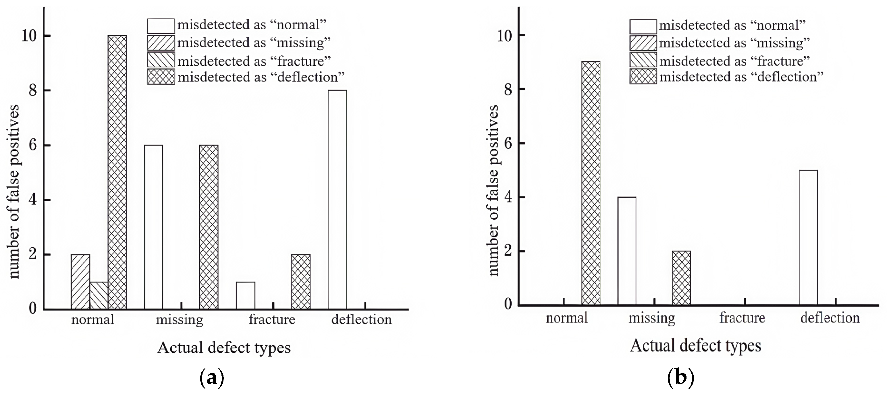
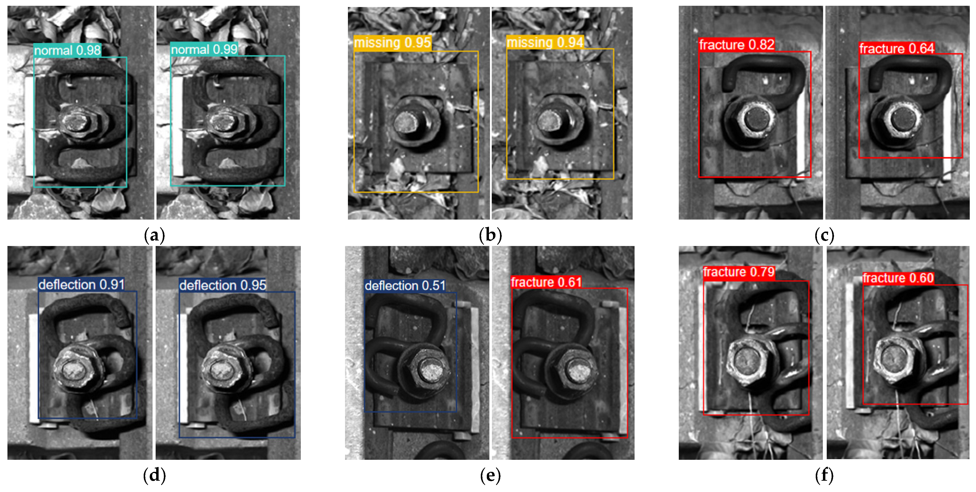
According to the defect types, the false detection situations of the model before and after improvement were counted, detailing the number of each defect type being misidentified as another defect type. The comparison results are shown in Figure 11. Using the improved YOLOv5 to infer 1300 fastener images for detection, the false detection rates of nut missing and clip missing defect types can be reduced to zero. The false detection rates of normal fastener and clip fracture are nearly halved compared to those before the model improvement, and the number of each defect type being misidentified as another defect type is fewer than the results inferred by the original YOLOv5m. As can be seen from Table 7, the improved model not only has a reduced size and faster detection speed but also significantly lowers the false detection rate. The partial comparison of fastener defect detection results using the pre-improvement and post-improvement models is shown in Figure 12. The enhanced model demonstrates significantly better performance than the baseline model. However, it still misidentifies some partially occluded fasteners as “fracture” defects. In the next research phase, we will prioritize improving detection performance for occluded targets.

5. Conclusions

This study addresses two critical challenges in rail fastener defect detection: the scarcity of specialized datasets and the inefficiency of existing detection algorithms. We establish a custom fastener dataset and propose an enhanced YOLOv5m-based approach for railway fastener defect inspection.
The proposed model incorporates dual-attention modules in the neck network and adopts CARAFE as the upsampling operator to extract richer feature representations, thereby enhancing focus on critical features. For lightweight construction, the backbone is replaced with MobileNetv3 while integrating GSConv modules into the YOLOv5m neck structure. Finally, the loss function is upgraded from CIOU to SIOU to accelerate convergence. Experimental validation confirms 96.5% mAP at 17.9 FPS—representing a 3.1 percentage-point improvement and 2.1 FPS gain over the baseline. The enhanced model also demonstrates heightened generalization capability and robustness.
Future research will prioritize tackling computational complexity and enhancing occlusion detection capabilities to address the observed phenomena of significant parameter reduction without proportional speed gains and difficulties in detecting occluded objects, while pursuing improved activation functions, alternative network architectures, and TensorRT deployment for accelerated inference and compact models, and implementing the system on inspection vehicles with industrial-grade cameras for real-time detection during railway track operation.

Author Contributions

D.L.: Methodology, Formal Analysis, Writing—Original Draft. J.M.: Conceptualization, Formal Analysis. G.M.: Investigation. Y.S.: Data curation. All authors have read and agreed to the published version of the manuscript.

Funding

This work was supported by the National Natural Science Foundation of China [No. 62363021] and Lanzhou Science and Technology Plan Project (Key) [16 January 2023].

Data Availability Statement

The data presented in this study are available on request from the corresponding author (the data comes from the railway department and is classified as confidential, hence it cannot be publicly accessed).

Conflicts of Interest

The authors declare no potential conflicts of interest with respect to the research, authorship, and/or publication of this article.

References

  1. Hasap, A.; Paitekul, P.; Noraphaiphipaksa, N.; Kanchanomai, C. Analysis of the fatigue performance of elastic rail clip. Eng. Fail. Anal. 2018, 92, 195. [Google Scholar] [CrossRef]
  2. Chellaswamy, C.; Krishnasamy, M.; Balaji, L.; Dhanalakshmi, A.; Ramesh, R. Optimized Railway Track Health Monitoring System Based on Dynamic Differential Evolution Algorithm. Measurement 2020, 152, 107332. [Google Scholar] [CrossRef]
  3. Maiwald, D.; Fass, U.; Litschke, H. Railcheck system: Automated optoelectronic inspection of rail systems. Eisenbahningenieur 1998, 7, 33. [Google Scholar]
  4. Zhang, W. Application of German RAILCHECK photoelectric automatic rail detection system in track inspection vehicles. Harbin Railw. Technol. 2001, 4, 3. (In Chinese) [Google Scholar]
  5. Stella, E.; Mazzeo, P.; Nitti, M.; Cicirelli, G.; Distante, A.; D’Orazio, T. Visual recognition of missing fastening elements for railroad maintenance. In Proceedings of the IEEE 5th International Conference on Intelligent Transportation Systems, Washington, DC, USA, 6 September 2002. [Google Scholar]
  6. Ma, H.; Min, Y.; Yin, C.; Cheng, T.; Xiao, B.; Yue, B.; Li, X. A Real Time Detection Method of Track Fasteners Missing of Railway Based on Machine Vision. Int. J. Perform. Eng. 2018, 14, 1190. [Google Scholar] [CrossRef]
  7. Gibert, X.; Patel, V.M. Sequential Score Adaptation with Extreme Value Theory for Robust Railway Track Inspection. In Proceedings of the IEEE International Conference on Computer Vision Workshops (ICCVW), Santiago, Chile, 7–13 December 2015. [Google Scholar]
  8. Gibert, X.; Patel, V.M.; Chellappa, R. Deep Multitask Learning for Railway Track Inspection. IEEE Trans. Intell. Transp. Syst. 2016, 18, 153. [Google Scholar] [CrossRef]
  9. Wei, X.; Yang, Z.; Liu, Y.; Wei, D.; Jia, L.; Li, Y. Railway Track Fastener Defect Detection Based on Image Processing and DeepLearning Techniques: A Comparative Study. Eng. Appl. Artif. Intell. 2019, 80, 66–81. [Google Scholar] [CrossRef]
  10. Liu, J.; Liu, H.C.; Chakraborty, K. Cascade learning embedded vision inspection of rail fastener by using a fault detection IoT vehicle. IEEE Internet Things J. 2021, 10, 1–11. [Google Scholar] [CrossRef]
  11. Wei, X.; Wei, D.; Suo, D.; Jia, L.; Li, Y. Multi-Target Defect Identification for Railway Track Line Based on Image Processing and Improved YOLOv3 Model. IEEE Access 2020, 8, 61973–61988. [Google Scholar] [CrossRef]
  12. Shiy, Y.; Shi, D.X.; Qiao, Z.T.; Zhang, Y.; Liu, S.; Yang, S. A survey on recent advances in few-shot object detection. Chin. J. Comput. 2023, 46, 1753. (In Chinese) [Google Scholar]
  13. Chen, J.W.; Liu, Z.G.; Wang, H.R.; Nunez, A.; Han, Z. Automatic defect detection of fasteners on the catenary support device using deep convolutional neural network. IEEE Trans. Instrum. Meas. 2018, 67, 257. [Google Scholar] [CrossRef]
  14. Wei, F.; Zhou, J.P.; Tan, X.; Lin, J.; Tian, L.; Wang, H. Lightweight YOLOv5 detection algorithm for low-altitude micro UAV. J. Optoelectron. 2024, 35, 641–649. [Google Scholar]
  15. Redmon, J.; Divvala, S.; Girshick, R.; Farhadi, A. You only look once: Unified, real-time object detection. arXiv 2015, arXiv:1506.02640. [Google Scholar]
  16. Hegbste, V.; Legler, T.; Ruskowski, M. Federated ensemble YOLOv5: A better generalized object detection algorithm. arXiv 2023, arXiv:2306.17829. [Google Scholar]
  17. Hu, J.; Shen, L.; Albanie, S.; Sun, G.; Wu, E.H. Squeeze-and-excitation networks. arXiv 2023, arXiv:1709.01507. [Google Scholar]
  18. Hou, Q.B.; Zhou, D.Q.; Feng, J.S. Coordinate attention for efficient mobile network design. arXiv 2021, arXiv:2103.02907v1. [Google Scholar] [CrossRef]
  19. Zhang, Y.; Lv, D.F.; Meng, J.J.; Qi, W.Z. Rail fastener defect detection based on dual attention and GSSN lightweighting. J. Comput. Eng. 2025, 51, 289–299. [Google Scholar]
  20. Howard, A.; Sandler, M.; Chou, G.; Chen, L.C.; Chen, B.; Tan, M.; Wang, W.; Zhu, Y.; Pang, R.; Vasudevan, V.; et al. Searching for MobileNetV3[EB/OL]. arXiv 2019. [Google Scholar] [CrossRef]
  21. Li, Y.D.; Han, Z.Q.; Xu, H.Y.; Liu, L.; Li, X.; Zhang, K. YOLOv3-Lite: A lightweight crack detection network for aircraft structure based on depthwise separable convolution. Appl. Sci. 2019, 9, 3781. [Google Scholar] [CrossRef]
  22. Chollet, F. Xception: Deep learning with depthwise separable convolutions. arXiv 2016, arXiv:1610.02357. [Google Scholar]
  23. Chen, Z.C.; Jiao, H.N.; Yang, J.; Zeng, H.F. Garbage image classification algorithm based on improved MobileNet v2. J. Zhejiang Univ. (Eng. Sci.) 2021, 55, 1490. (In Chinese) [Google Scholar]
  24. Hu, J.; Wang, Z.; Chang, M.; Xie, L.; Xu, W.; Chen, N. PSG-Yolov5: A Paradigm for Traffic Sign Detection and Recognition Algorithm Based on Deep Learning. Symmetry 2022, 14, 2262. [Google Scholar] [CrossRef]
  25. Li, H.L.; Li, J.; Wei, H.B.; Liu, Z.; Zhan, Z.; Ren, Q. Slim-neck by GSConv: A better design paradigm of detector architectures for autonomous vehicles. arXiv 2022, arXiv:2206.02424v1. [Google Scholar] [CrossRef]
  26. Wang, B.N. A parallel implementation of computing mean average precision. arXiv 2022, arXiv:2206.09504v1. [Google Scholar] [CrossRef]
  27. Gevorgyan, Z. SIoU loss: More powerful learning for bounding box regression. arXiv 2022, arXiv:2205.12740. [Google Scholar] [CrossRef]
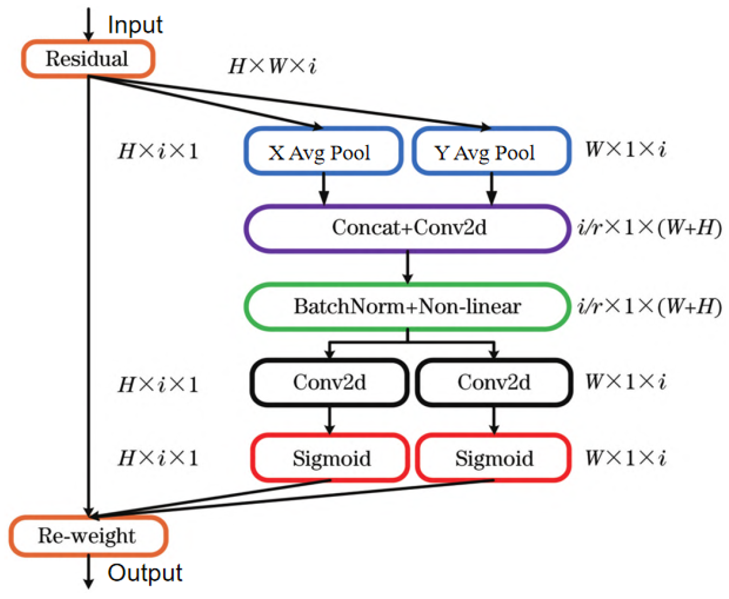
Figure 2. Working principle of CA mechanism.
Wevj 16 00513 g002
Figure 3. Structure of dual-attention mechanism.
Wevj 16 00513 g003
Figure 4. Structure of upsampling operator CARAFE.
Wevj 16 00513 g004
Figure 5. DSC process after GSConv.
Wevj 16 00513 g005
Figure 6. Structures of VoV-GSCSP and bottleneck. (a) VoV-GSCSP; (b) bottleneck.
Wevj 16 00513 g006
Figure 7. Model structure of modified YOLOv5m.
Wevj 16 00513 g007
Figure 8. Schematic diagrams of calculations of distance loss and angle loss. (a) Distance loss; (b) Angle loss. Reprinted with permission from Ref. [19]. Copyright 2025 Computer Engineering Editorial Office.
Wevj 16 00513 g008
Figure 9. Change trend of each index in process of model training. (a) box_loss; (b) obj_loss; (c) cls_loss; (d) mAP. Reprinted with permission from Ref. [19]. Copyright 2025 Computer Engineering Editorial Office.
Wevj 16 00513 g009
Figure 10. P-R curves of model before and after improvement. Reprinted with permission from Ref. [19]. Copyright 2025 Computer Engineering Editorial Office.
Wevj 16 00513 g010
Figure 11. Comparisons of false detections of pre- and post-improvement models. (a) Native YOLOv5m; (b) Improved YOLOv5. Reprinted with permission from Ref. [19]. Copyright 2025 Computer Engineering Editorial Office.
Wevj 16 00513 g011
Figure 12. Comparisons of partial effects of using pre- and post-improvement models for fastener defect detections. (a) normal, (b) missing, (c) fracture, (d) deflection, (e) fracture error, (f) deflection error. Adapted with permission from Ref. [19]. Copyright 2025 Computer Engineering Editorial Office.
Wevj 16 00513 g012
Table 1. The number of fastener images for different working conditions in the training set.
TypesNormalMissingFractureDeflection
Number2680135612111253
Table 2. Experimental hyperparameter settings.
Hyperparameter NameHyperparameter Value
Input Image Size640 × 640
Initial Learning Rate0.005
Training Epochs300
Warmup Learning Rate Momentum0.937
Bounding Box Localization Loss Coefficient0.05
Classification Loss Coefficient0.5
Confidence Loss Coefficient0.5
Mosaic Data Augmentation Ratio1
Batch Size Normalization Value16
Table 3. Comparison of results of using different backbone networks.
BackboneP/% R/% AmAP/% GPU Memory Usage (GB)
CSPDarkNet (Baseline)89.992.394.54.53
ShuffleNetv275.685.087.83.49
MobileNetv275.892.288.03.95
MobileNetv3 (Proposed)76.395.688.33.70
Table 4. Comparisons of results of using different attention mechanisms.
Attention MechanismsP/% R/% AmAP/% GPU Memory Usage (GB)
SE (Original)89.992.394.54.53
CBAM92.994.497.34.92
Dual Attention (Neck)90.792.994.84.50
Dual Attention
(Backbone, Ours)
95.996.398.94.45
Table 5. Comparisons of results of using different coordinate loss functions.
Coordinate Loss FunctionsP/% R/% AmAP/% GPU Memory Usage (GB)
CIoU (Original)89.992.394.54.53
DIoU91.493.396.74.53
GIoU96.095.297.74.53
SIoU (Ours)96.195.897.74.53
Table 6. Results of ablation experiments. Reprinted with permission from Ref. [19]. Copyright 2025 Computer Engineering Editorial Office.
MobileNetv3GSSNDual AttentionCARAFESIoUP/%R/%AmAP/%GPU Memory Usage (GB)Model Size/MB
×××83.592.992.33.749.1
×××77.888.788.73.246.9
×××75.490.988.63.317.5
×××83.392.492.33.749.1
××84.495.194.03.658.3
××88.489.895.23.749.1
×88.995.596.13.658.3
89.296.096.53.598.3
Table 7. Comparison of detection performance between pre- and post-improvement models and other major models. Adapted with permission from Ref. [19]. Copyright 2025 Computer Engineering Editorial Office.
AlgorithmP/%R/%mAP50/%mAP
50–95/%
GPU Memory Usage (GB)GFLOPs
(G)
Param
(M)
FPS
YOLOv5m
(Baseline)
92.791.593.476.94.5320.949.115.79
Faster-RCNN81.483.082.871.56.95112.1131.59.21
SSD83.184.484.771.95.253490.210.12
YOLOv390.991.892.474.35.8561.6156.49.93
YOLOv492.191.992.875.75.9269.6195.111.83
YOLOv4-tiny90.091.191.874.53.775.95.617.23
Improved YOLOv596.195.296.577.63.656.537.317.90
Disclaimer/Publisher’s Note: The statements, opinions and data contained in all publications are solely those of the individual author(s) and contributor(s) and not of MDPI and/or the editor(s). MDPI and/or the editor(s) disclaim responsibility for any injury to people or property resulting from any ideas, methods, instructions or products referred to in the content.