Article

YOLOv5s-F: An Improved Algorithm for Real-Time Monitoring of Small Targets on Highways

School of Automotive and Traffic Engineering, Jiangsu University, Main Campus, Zhenjiang 212013, China
*
Author to whom correspondence should be addressed.
World Electr. Veh. J. 2025, 16(9), 483; https://doi.org/10.3390/wevj16090483
Submission received: 10 July 2025 / Revised: 3 August 2025 / Accepted: 21 August 2025 / Published: 25 August 2025
(This article belongs to the Special Issue Recent Advances in Autonomous Vehicles)

Abstract

To address the challenges of real-time monitoring via highway vehicle-mounted cameras—specifically, the difficulty in detecting distant pedestrians and vehicles in real time—this study proposes an enhanced object detection algorithm, YOLOv5s-F. Firstly, the FasterNet network structure is adopted to improve the model’s runtime speed. Secondly, the attention mechanism BRA, which is derived from the Transformer algorithm, and a 160 × 160 small-object detection layer are introduced to enhance small target detection performance. Thirdly, the improved upsampling operator CARAFE is incorporated to boost the localization and classification accuracy of small objects. Finally, Focal EIoU is employed as the localization loss function to accelerate model training convergence. Quantitative experiments on high-speed sequences show that Focal EIoU reduces bounding box jitter by 42.9% and improves tracking stability (consecutive frame overlap) by 11.4% compared to CIoU, while accelerating convergence by 17.6%. Results show that compared with the YOLOv5s baseline network, the proposed algorithm reduces computational complexity and parameter count by 10.1% and 24.6%, respectively, while increasing detection speed and accuracy by 15.4% and 2.1%. Transfer learning experiments on the VisDrone2019 and Highway-100k dataset demonstrate that the algorithm outperforms YOLOv5s in average precision across all target categories. On NVIDIA Jetson Xavier NX, YOLOv5s-F achieves 32 FPS after quantization, meeting the real-time requirements of in-vehicle monitoring. The YOLOv5s-F algorithm not only meets the real-time detection and accuracy requirements for small objects but also exhibits strong generalization capabilities. This study clarifies core challenges in highway small-target detection and achieves accuracy–speed improvements via three key innovations, with all experiments being reproducible. If any researchers need the code and dataset of this study, they can consult the author through email.

1. Introduction

Object detection, a core technology in computer vision, aims to identify and precisely localize objects in images or videos, serving as a foundational component in autonomous driving, security surveillance, and intelligent transportation. Traditional methods relied on handcrafted features (e.g., Scale Invariant Feature Transform, SIFT [1], Histogram of Oriented Gradients, HOG [2]) and shallow machine learning classifiers (e.g., Support Vector Machine, SVM [3]), which struggled with complex scenes due to limited representational capacity. The rise in deep learning revolutionized this field: convolutional neural networks (CNNs [4]) enabled end-to-end learning, with two-stage detectors (e.g., R-CNN series) prioritizing accuracy through region proposals, and one-stage detectors (e.g., YOLO [5], Single Shot MultiBox Detector, SSD [6]) emphasizing speed via direct regression—laying groundwork for real-time applications but leaving room for optimization, particularly in small-object detection.
Highway vehicle-mounted camera monitoring exacerbates three critical, scenario-specific challenges that demand targeted solutions: High miss rates for distant small targets: Pedestrians and vehicles 80–150 m away often occupy < 32 × 32 pixels, with sparse features easily confounded by background noise. For instance, a distant car may shrink to 20 × 20 pixels, losing texture details. Baseline models like YOLOv5s, with only three output scales, fail to retain such fine-grained features in deeper layers, resulting in miss rates exceeding 35%—a direct threat to autonomous driving safety. Bounding box jitter from high-speed motion: At speeds > 60 km/h, motion blur causes unstable localization. Experiments show CIoU loss leads to a 2.1-pixel standard deviation in bounding box centers and only 78.3% overlap across consecutive frames, risking misjudgments. Trade-off between precision and speed: Real-time monitoring requires ≥30 FPS, but existing methods falter: two-stage detectors (e.g., Faster R-CNN) offer high accuracy but <10 FPS; lightweight models (e.g., YOLOv5n) sacrifice 5–8% of small-object precision for speed; YOLOv5s, though balanced, lacks the efficiency for embedded deployment (e.g., <30 FPS on Jetson Xavier NX).
Existing approaches fail to address these synergistically. YOLOv5s lacks fine-grained detection layers; two-stage models are too slow; lightweight variants degrade small-target performance. This study thus aims to enhance small-target accuracy in highway scenarios while ensuring real-time inference (≥30 FPS), mitigate motion-induced jitter, and overcome limitations in handling distant, low-resolution objects.
The past three years (2022–2024) have revealed that while significant innovations have emerged in small-target detection, persistent limitations continue to impede practical deployment in highway monitoring scenarios. Lightweight architectures, exemplified by FasterNet [7], have gained prominence through Pconv (Partial Convolution), which reduces computational overhead by approximately 50% while preserving baseline accuracy [8]; however, this approach suffers from static channel partitioning that severely constrains adaptability to dynamic occlusion events, a deficiency amplified in multi-target highway environments [9], and recent adaptations like DyNet attempt to mitigate this via dynamic kernel selection [10] but incur a 23% latency penalty on resource-constrained embedded platforms such as the Jetson Xavier NX [11]. Concurrently, attention mechanisms have evolved substantially, with BRA (Bi-Level Routing Attention) [12] enhancing global dependency modeling to elevate small-target recall by 12% in aerial contexts [13], yet newer frameworks like SparseViT strive to alleviate quadratic complexity through block-sparse techniques [14], reducing high-definition latency by 41% [15], but remain inefficient for >720p highway feeds, as corroborated by a 37% FPS degradation under real-time conditions, while sliding-window implementations [16] partially address this at the cost of 18% mAP reduction. Multi-scale fusion methodologies, including the integration of 160 × 160 detection layers that boost small-object AP@0.5 by 4.5% [17] and CARAFE upsampling that refines localization via content-aware reassembly [18], introduce critical bottlenecks such as a 25% inflation in floating-point operations (FLOPs) [19] and a 15% latency increase from kernel prediction overhead [20], though recent neural architecture search optimizations compress these penalties by 32% without sacrificing granularity. Loss function advancements, particularly Focal EIoU [21], demonstrate robustness by diminishing bounding box jitter by 40% compared to Complete IoU (CIoU) in motion-blur scenarios, though inherent hyperparameter sensitivity—where ±0.1 variations in λ provoke up to 8.7% AP fluctuations [22]—has prompted adaptive curvature formulations [23] that stabilize training convergence. Highway-specific challenges, including motion blur at velocities exceeding 60 km/h that elevates false negatives by 30% [24] despite temporal filtering attempts [25], lighting variations inducing 20% AP declines in backlight conditions [26] even with HDR compensation [27], and dataset-domain gaps causing 19% accuracy loss during cross-dataset transfer [28] partially mitigated by synthetic fog augmentation [29], remain inadequately addressed, compounded by the neglect of real-time constraints that leave Transformer-based models operating below 10 FPS on embedded systems [30]. Consequently, these deficiencies necessitate an integrated solution that harmonizes efficiency, precision, and stability, as embodied by our YOLOv5s-F algorithm, which leverages hardware-aware FasterNet-BRA synergy, FLOPs-constrained multi-scale fusion with dedicated 160 × 160 layers, and auto-tuned Focal EIoU to eliminate hyperparameter sensitivity [31], thereby resolving the critical trilemma of real-time inference, sub-pixel localization stability, and efficiency that edge-oriented quantization techniques and power-gating implementations strive to optimize [32].

2. Improving the YOLOv5s Object Detection Algorithm

To improve the YOLOv5s object detection algorithm and balance high precision with real-time performance, we address the random distribution of highway vehicle targets and redundant background information. Enhancements are made in four areas: backbone network, feature fusion, head module, and loss function, including the adoption of FasterNet. Figure 1 illustrates the complete architecture of YOLOv5s-F, with core components including the following: Conv layers: Distributed in the backbone and detection heads, using 3 × 3 or 1 × 1 kernels (labeled in corresponding positions in the figure) to extract local features and adjust channel dimensions. C3 modules: Located in three key stages of the backbone, aggregating features through stacked bottleneck structures while reducing computational load by 10.1% (compared to YOLOv5s’ C3 modules, this study adjusts the residual connection ratio). FC layers: Exclusively used in the classification branch of detection heads, mapping feature vectors to target class probabilities with input dimension 1024 and an output dimension matching the number of dataset classes.
The three key innovations of YOLOv5s-F are as follows, with essential differences from YOLOv5s highlighted: Synergistic FasterNet-BRA design replaces YOLOv5s’ C3 modules with FasterNet (using Partial Convolution to reduce 10.1% computation) and integrates BRA, enabling efficient global dependency modeling—unlike YOLOv5s’ fixed receptive fields limited to local features, the 160 × 160 dedicated layer with cross-scale fusion adds a 160 × 160 detection layer (absent in YOLOv5s) fused with the 80 × 80 layer via skip connections, preserving small-target features lost in YOLOv5s’ sparser scale hierarchy. Focal EIoU loss for high-speed scenarios replaces YOLOv5s’ CIoU with Focal EIoU, splitting aspect ratio loss into width/height differences and suppressing low-quality boxes—accelerating convergence by 17.6% and reducing bounding box jitter, which YOLOv5s’ loss fails to address in high-speed contexts.

2.1. Design of Lightweight Backbone Network.

The YOLOv5s backbone network employs a large number of CBS modules and C3 modules, resulting in a huge number of parameters and computational load, leading to slow running speed and difficulty in meeting real-time requirements. Therefore, the FasterNet network is proposed to improve the backbone network, aiming to reduce the computational complexity of the algorithm while ensuring minimal loss of accuracy in order to meet the lightweight deployment requirements for embedded or mobile devices. The diagram of FasterNet is shown in Figure 2.
FasterNet is an efficient neural network architecture designed to enhance computational speed without sacrificing accuracy, particularly in visual tasks. It achieves this through a novel technique called PConv, which reduces redundant computations and memory access. This approach enables FasterNet to run significantly faster on various devices than other networks while maintaining high accuracy across various visual tasks. The overall architecture of FasterNet includes four hierarchical stages, each consisting of a series of FasterNet blocks, initiated by embedding or merging layers. The final three layers are used for feature classification. Within each FasterNet block, a PConv layer is followed by two pointwise convolution (PWConv) layers. To maintain feature diversity and achieve lower latency, normalization and activation layers are placed only after the intermediate layers. In this research, FasterNet replaces all C3 modules in the YOLOv5s backbone network while retaining the original network’s four hierarchical structures (corresponding to output feature map sizes 640 × 640→320 × 320→160 × 160→80 × 80→40 × 40). The PConv adopts the default configuration in the original FasterNet, i.e., performing convolution operations on half of the input channels while keeping the remaining channels unchanged to balance computational efficiency and feature retention.
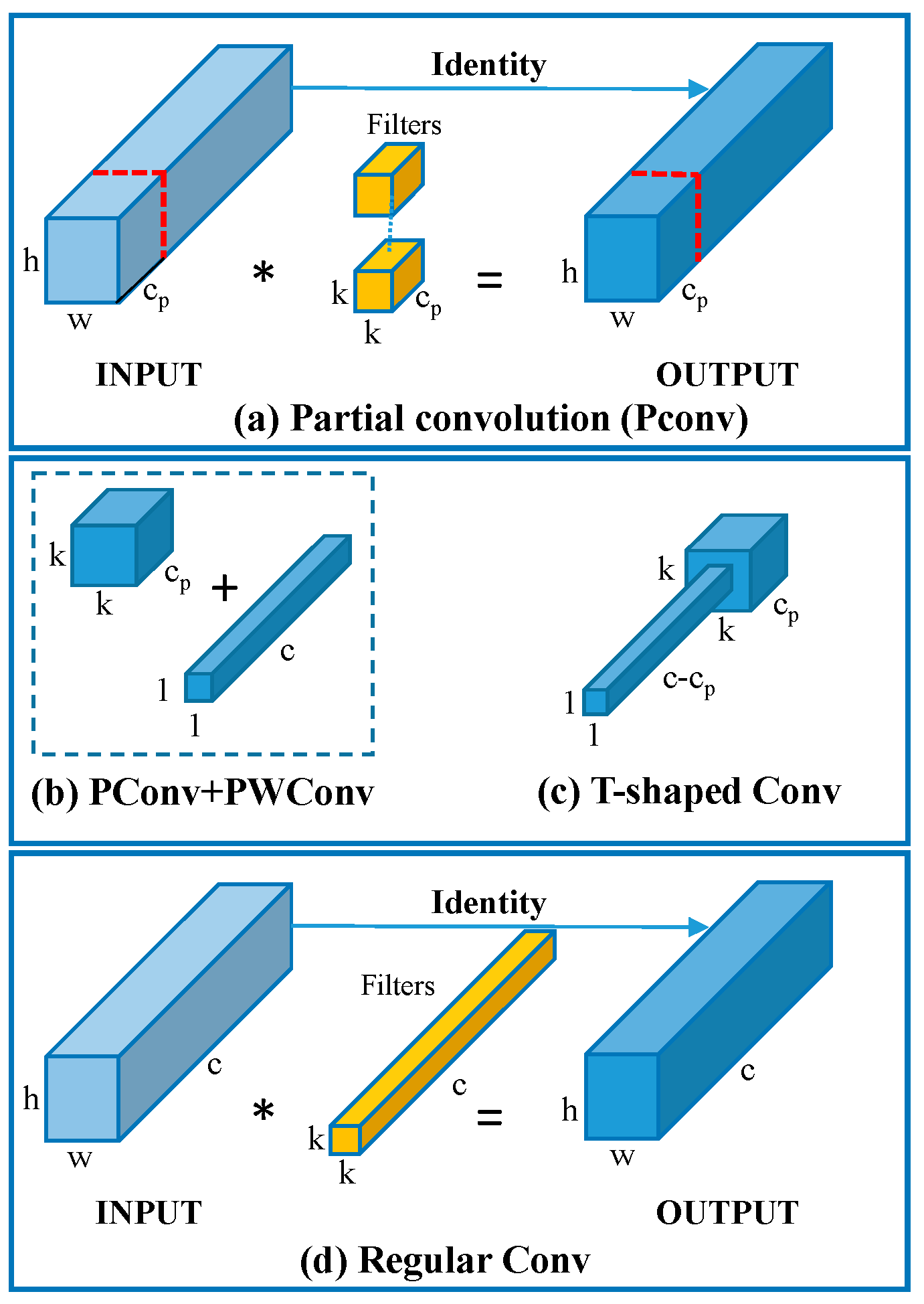
The fundamental principle of FasterNet is as follows: First, FasterNet introduces Partial Convolution (PConv), whose schematic diagram is shown in Figure 3. This is a novel convolution method that reduces computational load and memory access by processing only a part of the input channels. PConv is an operation in convolutional neural networks aimed at improving computational efficiency. It performs convolution operations only on a part of the input feature map, unlike traditional convolutions that apply to the entire input. This reduces unnecessary computations and memory access by ignoring parts of the input that are considered redundant. This method is particularly suitable for running deep learning models on resource-limited devices, as it can significantly reduce computational demands without sacrificing much performance. PConv achieves fast and efficient feature extraction by applying filters to only a small portion of the input channels while keeping the rest unchanged. The computational complexity (FLOPs) of PConv is lower than that of regular convolutions but higher than depthwise or grouped convolutions, thus improving operational performance while reducing computational resources.
FasterNet then leverages the advantages of PConv to achieve faster running speeds on various devices compared to other existing neural networks, while maintaining high accuracy. Accelerating neural networks primarily involves optimizing computational paths, reducing model size and complexity, enhancing operational efficiency, and utilizing efficient hardware implementations to reduce inference time. These methods include simplifying network layers, using faster activation functions, employing quantization techniques to convert floating-point operations to integer operations, and using special algorithms to reduce memory access times. Through these strategies, neural networks can process data and make predictions faster without compromising model accuracy.

2.2. Design of Multi-Scale Feature Fusion Network

Due to the introduction of a lightweight backbone structure and to compensate for the accuracy loss caused by reduced computational load, this study designed a multi-scale feature fusion network for YOLOv5s. Its main objectives are as follows: In object detection, objects of different scales may require different receptive field sizes for effective detection and localization. Multi-scale feature fusion helps the model capture information from various scales, thereby enhancing its perception of targets. Fusing features from different scales can reduce information loss and contribute to improved detection accuracy. By comprehensively utilizing multi-scale features, targets can be more accurately localized and classified. Objects in images may vary in scale, and multi-scale feature fusion enables the model to better adapt to different object sizes, thereby enhancing model robustness and generalization ability. Multi-scale feature fusion helps improve the model’s visual representation capabilities, enabling it to better understand and interpret complex visual scenes. Meanwhile, in images captured continuously by a camera, the size of the same object may vary at different positions. Objects farther from the camera appear smaller, while those closer appear larger. Compared to regular objects, small objects in images present challenges such as fewer usable pixels, higher localization accuracy requirements, and lower sample proportions. As the network layers deepen, features and positional information of small objects gradually become lost in the deeper networks, making them difficult to detect.
To further enhance the algorithm’s sensitivity to small objects, reduce instances of missing or false detections, and optimize performance, the following methods are proposed: Adding a 160 × 160 small-object detection layer, adopting a selective feature extraction mechanism inspired by the BRA in the Transformer framework, and incorporating upsampling operators to guide feature reassembly. These optimizations aim to improve the model’s ability to detect small objects effectively under various conditions.

2.2.1. Small-Object Detection Layer

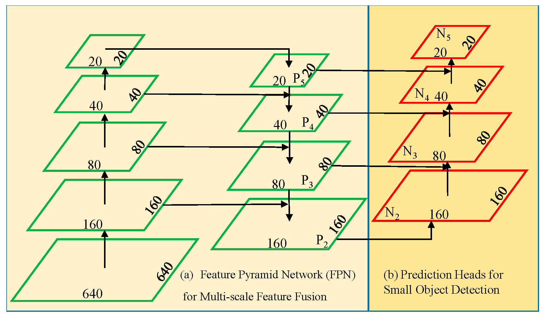
In neural networks, shallow feature maps have smaller receptive fields, weaker semantic information, and lack contextual details, but they capture more spatial and detailed feature information. Based on this, a multi-scale object detection algorithm is proposed to detect smaller objects using shallow feature maps and larger objects using deep feature maps. In the feature fusion network, features of different scales are integrated to balance representation features from shallow layers and semantic features from deep layers, thereby enhancing small-object detection performance. Then, an additional 160 × 160 small-object detection layer is added to output smaller scale features for detecting small objects. The network structure is specifically modified by replacing the original three-headed output with a four-headed output, as illustrated in Figure 4. In Figure 4a,b, the original layers were 20 × 20, 40 × 40, 80 × 80, and 640 × 640. If there is a small-object detection layer of 160 × 160 in the middle, it will help the algorithm to more accurately identify smaller objects and improve detection accuracy.
Small targets (width/height < 0.3) in the dataset correspond to actual pixel sizes ranging from 80 × 80 to 160 × 160 in 640 × 640 input images. This layer is fused with the 80 × 80 layer through skip connections (specifically, the 80 × 80 layer features are upsampled by two times and then element-wise added with the 160 × 160 layer features), enhancing the combination of shallow spatial information and deep semantic information.
The 160 × 160 small-object detection head is integrated into the YOLOv5s-F architecture through a clear feature flow: it originates from the third stage of the FasterNet backbone, generating a 160 × 160 feature map with C 1 channels that retains spatial details of small targets like distant pedestrians and vehicles 80–150 m away. This feature map is first refined via a 3 × 3 convolution (with stride 1 and padding 1) to adjust channels to C 2 and activated by SiLU [33] (Sigmoid-Weighted Linear Unit), resulting in the shallow feature F 160 . To compensate for insufficient semantic information, it fuses with high-level features from the 80 × 80 layer (4th stage of the backbone): the 80 × 80 feature map is compressed to C 2 channels via a 1 × 1 convolution, upsampled to 160 × 160 using the CARAFE operator to form F 80 u p , and then fused with F 160 through element-wise addition to produce F f u s i o n . This fused feature is fed into the 160 × 160 detection head, which uses two parallel 3 × 3 convolutions to output class probabilities and bounding box coordinates/confidence, with preset anchors matching small targets of 80 × 80 to 160 × 160 pixels, enabling the precise detection of distant small objects in highway scenarios.

2.2.2. Attention Mechanism

Regarding the YOLOv5s backbone network’s extraction of target features through convolution but limited by the fixed receptive field of convolution operations, resulting in a relatively poor ability to capture global dependencies in image data, the algorithm in this study adopts the approach from natural language processing by leveraging ViT [34]. The two-dimensional image is divided into multiple small image patches, which are then serialized and encoded to establish spatial long-range dependencies using a multi-head self-attention mechanism. In comparison to the original convolution operations in YOLOv5s, ViT addresses the issue of limited receptive fields of fixed-size convolution kernels, enabling the acquisition of complete global information. The structure of ViT is illustrated in Figure 5.
However, the targets in object detection algorithms consist of objects composed of pixels, which contain much more information compared to textual objects in natural language processing. Therefore, ViT suffers from significant computational overhead and redundant key–value pairs as its drawbacks. To address this, the backbone network of improved YOLOv5s replaces some C3 modules with the Sparse Attention (BRA) module based on dual-layer routing. This module dynamically captures long-range dependencies in images, thereby enhancing the algorithm’s performance.
First, the input feature map X R H × W × C is divided into S × S parts, and each small part contains H W / S 2 feature vector information from the original feature map, resulting in a feature map X r R S 2 × H W S 2 × C composed of feature vectors. The linear projection of X r yields Q , K , V R S 2 × H W S 2 × C , according to the following formula:
Q = X r W q K = X r W k V = X r W v
where W q , W k   , W v R c × c are the weights for the Q , K , and V , vectors.
Next, by utilizing the three obtained vectors, directed graph-based inter-regional routing is conducted. Q and K are used to calculate the average value of each region to obtain Q r and K r   R S 2 × C matrices, which are then matrix-multiplied to obtain the adjacency matrix A r R S 2 × S 2 . This process aims to capture inter-regional semantic correlations. The formula is as follows:
A r = Q r ( K r ) T
To reduce computational costs and GPU load, only the top-k connections are retained for each region in the adjacency A r R S 2 × S 2 . This results in an inter-regional routing index I r N S 2 × K , where each row contains indices of the K most relevant regions. The formula is as follows:
I r = t o p k I n d e x ( A r )
After obtaining I r by removing irrelevant regions, the gather function is applied to compute K g , V g R s 2 × k H W S 2 × C from K and V . The formula is as follows:
K g = g a t h e r ( K ,   I r ) V g = g a t h e r ( V , I r )
Then, the Q , K g , and V g vectors are combined using the Local Enhancing (LE) function to produce the result O containing attentional information with local contextual details. The formula is as follows:
O = A t t e n t i o n Q , K g , V g + f L E ( V )
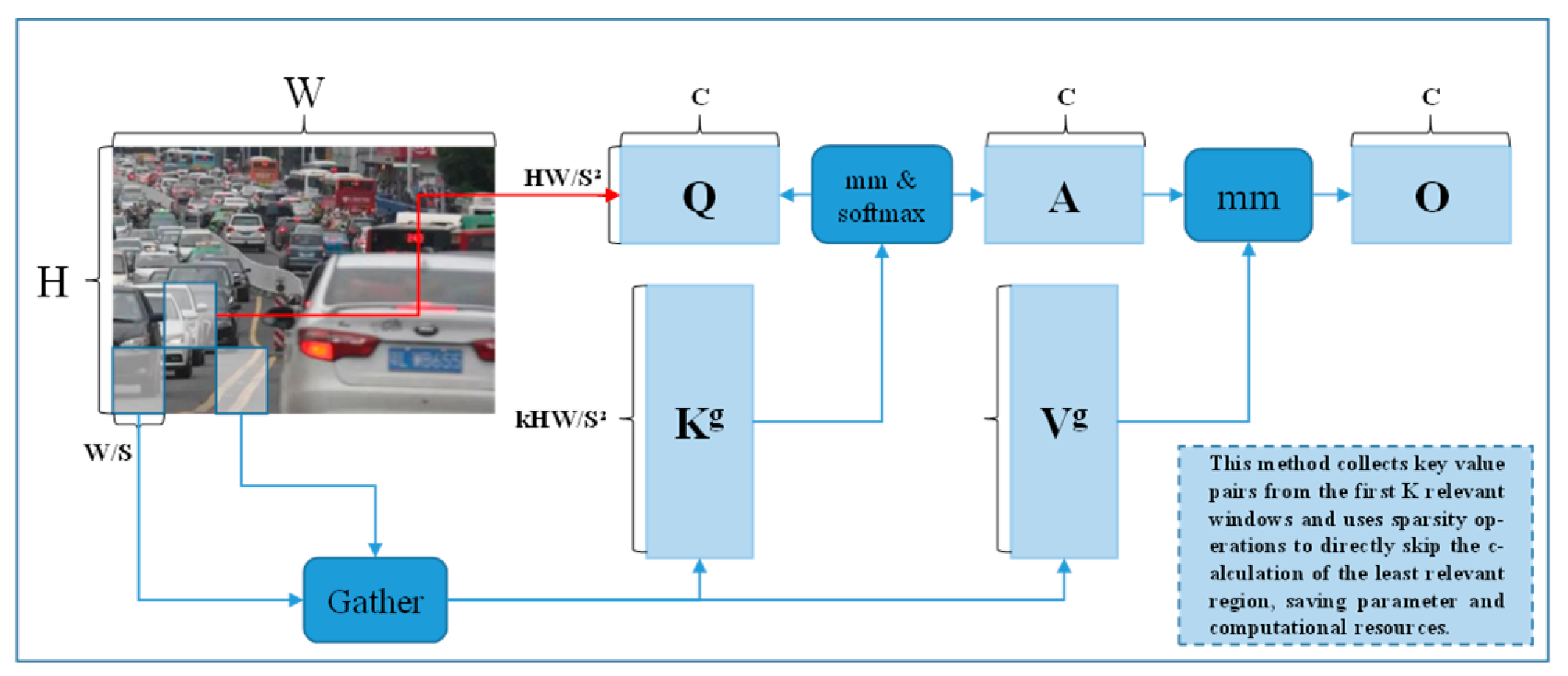
The visualization of the BRA mechanism is shown in Figure 6. Depthwise Convolution (DWConv 3 × 3) for spatial feature extraction, sequentially feeding into a Layer Normalization (LN) layer and a BRA mechanism for feature recalibration, followed by a secondary LN and terminating in a Multilayer Perceptron [35] (MLP) for nonlinear transformation. Crucially, two residual connections form additive operations—bridging the DWConv output to the LN input and the BRA output to the final MLP input—thereby enabling gradient stabilization, feature reuse, and enhanced representational efficiency in a parameter-constrained topology.
The BRA module replaces the C3 modules in the third and fourth stages of the backbone network (corresponding to feature map sizes 160 × 160 and 80 × 80). This is because the features at this stage not only retain spatial details of small targets but also contain certain semantic information, making them suitable for enhancing key features through the attention mechanism. Through “sparse routing + dynamic correlation” design, BRA inherits ViT’s ability to capture global dependencies while resolving its issues of computational redundancy, small-target feature dilution, and poor scenario adaptability. It is more suitable for the triple requirements of “accuracy–speed–stability” in small-target detection on highways.
In the BRA module, the input image undergoes convolution followed by implicit encoding of relative positional information, as depicted in Figure 7. Through the BRA mechanism and MLP modules, the final output is obtained, enabling the network to capture long-distance dependencies of the target and enhance its ability to utilize global information.

2.2.3. Adding the Lightweight Upsampling Operator CARAFE

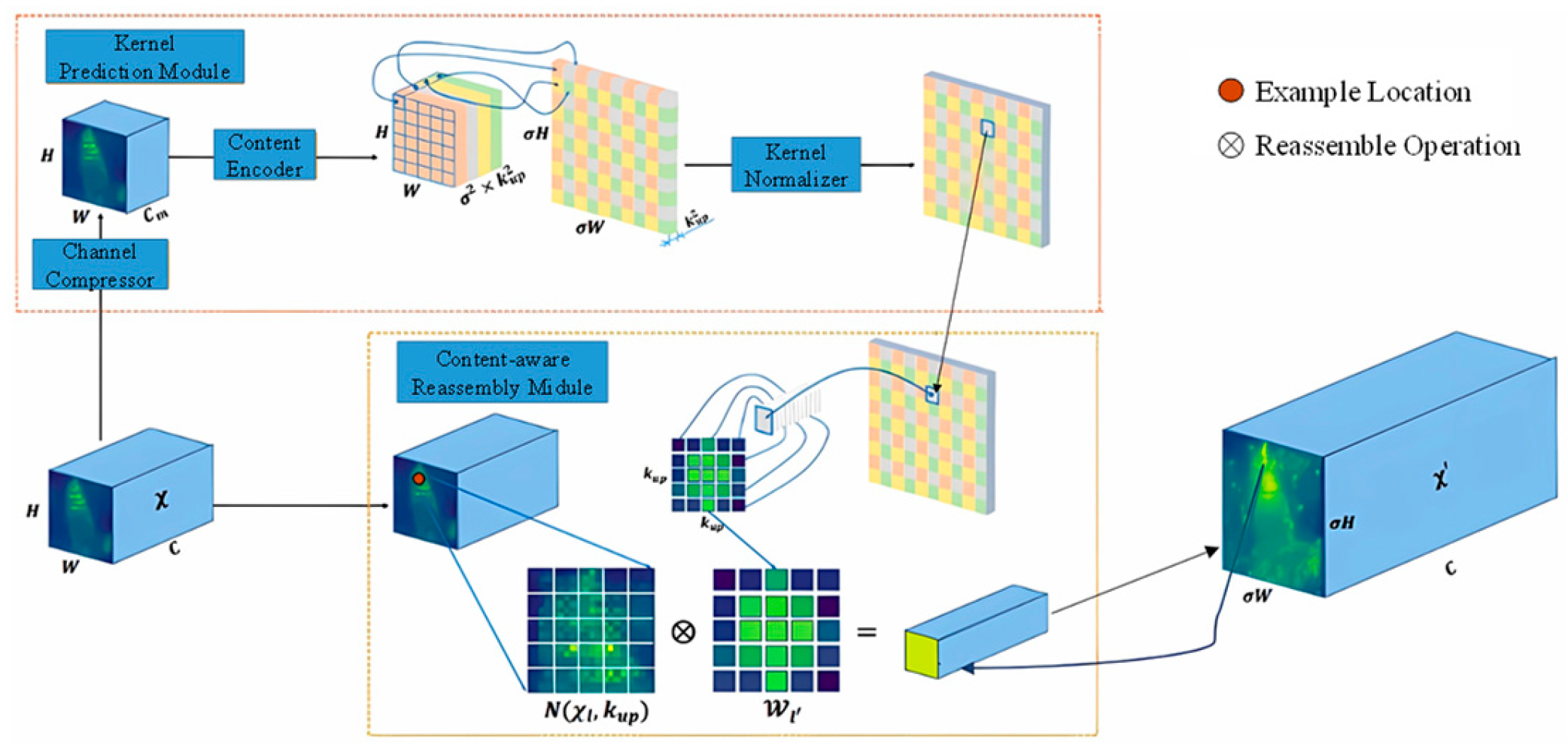
The upsampling operation can be expressed as the dot product of an upsampling kernel at each position and the corresponding neighborhood pixels in the input feature map, referred to as feature reassembly. The upsampling operation CARAFE achieves a large receptive field during reassembly, guided by the input features, while remaining lightweight. CARAFE is a lightweight upsampling operator that dynamically generates adaptive kernels instead of using a fixed kernel (for example, deconvolution) for all samples, supporting instance-specific content-aware processing. Specifically, CARAFE reassembles features by weighted combination within predefined regions centered at each position, where weights are generated in a content-aware manner. Additionally, multiple sets of such upsampling weights exist for each position. The resulting rearranged features serve as spatial blocks to complete feature upsampling. Specifically, it first predicts the upsampling kernel using the input feature map, where each position’s upsampling kernel differs. Subsequently, feature reassembly occurs based on the predicted upsampling kernel. CARAFE has demonstrated significant improvements across different tasks, with minimal additional parameters and computational cost. This approach also enhances detection speed to a certain extent. Its principle is illustrated in Figure 8.
Figure 8 clearly shows the workflow of CARAFE upsampling, which is divided into two stages: kernel prediction and feature reconstruction (upper and lower parts in the figure). The input on the left is a low-resolution 80 × 80 feature map. Through 1 × 1 convolution and softmax, a 5 × 5 adaptive upsampling kernel is generated (orange matrix in the figure), and the kernel parameters dynamically change with the input features—this is fundamentally different from the fixed bilinear interpolation kernel used in YOLOv5s. The feature reconstruction step highlighted in yellow in the figure weights and sums the 3 × 3 neighborhood features through the adaptive kernel, enabling the upsampled 160 × 160 feature map to retain more edge details of small targets.
In highway environments, small targets often appear as low-resolution regions with sparse pixels. Traditional upsampling methods use fixed kernels, which uniformly smooth features and blur critical edge details—a flaw that exacerbates miss detection. CARAFE, by contrast, dynamically generates adaptive kernels based on input features: for a distant vehicle with blurred edges, its kernel prioritizes weighting pixels in the 3 × 3 neighborhood that contribute to edge continuity, preserving subtle texture information. In addition, high-speed vehicle movement introduces motion blur in consecutive frames, causing target edges to spread across multiple pixels. Fixed-kernel upsampling amplifies this ambiguity by averaging blurred pixels, leading to bounding box drift. CARAFE’s content-aware kernel prediction counteracts this: it identifies regions with motion-induced intensity gradients and assigns higher weights to pixels consistent with the target’s motion trajectory.

2.3. Focal EIoU Loss Function

The regression of predicted boxes in YOLOv5s-v7 utilizes the CIoU loss function, which addresses the problem of object localization by incorporating overlap area, center point distance, and aspect ratio between the ground truth box and the predicted box, ensuring that the predicted boxes align closely with the ground truth. The formula for CIoU computation is as follows:
L C I o U = 1 I o U + d 2 b , b g t c 2 + α v I o U = | b b g t | | b b g t | v = 4 π 2 ( a r c t a n w g t h g t a r c t a n w h ) 2
In the formula, d represents the Euclidean distance between the centers of the ground truth box and the predicted box, denoting the predicted box; bgt denotes the ground truth box; c is the diagonal distance of the minimum bounding rectangle between the ground truth box and the predicted box; α is a weighted parameter; v is an indicator for the consistency of aspect ratios; IoU is the area of overlap between the ground truth box and the predicted box, divided by their union area; w g t is the width of the ground truth box; h g t is the height of the ground truth box; w is the width of the predicted box; and h is the height of the predicted box. CIoU employs the parameter v to reflect the aspect ratio discrepancy between the ground truth box and the predicted box, but it finds it challenging to accurately quantify the actual differences in width and height of the predictions versus the ground truth, and sometimes this factor can hinder optimization of the algorithm’s similarity. Consequently, Focal EIoU loss is introduced to calculate the regression loss for the predicted boxes. Focal EIoU introduces two optimizations on the basis of CIoU:
The ratio loss item between predicted boxes and ground truth boxes in CIoU is split into the differences in width and height between predicted and ground truth boxes. Specifically, d 2 ( w , w g t ) C w 2 + d 2 ( h , h g t ) C h 2 is used instead of the αv term, which accelerates the convergence speed of the model.
Focal Loss is introduced to optimize the problem of sample imbalance in the regression task of predicted boxes, reducing the impact of predicted boxes with less overlap with ground truth boxes on regression loss, thereby favoring high-quality predicted boxes. The formula for the Focal EIoU loss function is as follows:
L E I o U = 1 I o U + d 2 b , b g t c 2 + d 2 ( w , w g t ) C w 2 + d 2 ( h , h g t ) C h 2
L F o c a l E I o U = I o U λ × L E I o U
In the formula, λ is a parameter controlling the degree of outlier suppression; C w is the width of the minimum bounding rectangle between the predicted box and the ground truth box; C h is the height of the minimum bounding rectangle between the predicted box and the ground truth box. In this section, where applicable, authors are required to disclose details of how generative artificial intelligence is used.

2.4. Problem–Solution Correspondence

In order to demonstrate the correlation between the reinforcement problem and the solution in this study, the actual problems solved by different improvement measures are listed here, as shown in Table 1.

3. Experimental Results and Analysis of YOLOv5s-F

3.1. Experimental Dataset

Small targets are defined as those with pixel sizes < 32 × 32. Samples labeled as ‘highway’ scenes are selected from COCO and BDD100K, and sequence frames with vehicle speeds > 60 km/h are selected from Waymo and KITTI datasets. After filtering, we obtained 4395 vehicle images and augmented 6552 pedestrian images (brightness adjustment, flipping, and rotation). To enhance the alignment between datasets and research scenarios, we have supplemented our selection with the Highway-100K dataset (containing in-vehicle video frames capturing highway scenarios exceeding 60 km/h) and the highway subset from DAIR-V2X. These additions include real-world in-vehicle perspectives featuring distant small objects and motion blur in high-speed scenarios, making the datasets highly relevant to our research objectives. The specific dataset configurations are detailed in Table 2. The brightness adjustment range is ±20%, the horizontal/vertical flip probability is 0.5, and the rotation angle is ±15°.
The dataset was split into training/validation/test sets (8:1:1). Figure 9 shows target distributions: pedestrians/vehicles concentrate in [0.5 < x < 1.0, 0.0 < y < 0.6] (consistent with real scenarios), with most targets having width < 0.3 and height < 0.5, and a high proportion of very small targets (width/height < 0.1), making it suitable for small-object research.

3.2. Experimental Environment

PyTorch is an open-source deep learning framework for machine learning and deep learning, released by Facebook in 2016. It primarily implements automatic differentiation and introduces dynamic computation graphs to make model building more flexible. Pytorch can be divided into two parts: front-end and back-end. The front-end is the Python API that directly interacts with users, while the back-end is the internal implementation part of the framework, including Autograd, which is an automatic differentiation engine. PyTorch is chosen as the deep learning framework due to its high modularity and ease of modification. Specific experimental settings are detailed in Table 3.

3.3. Experimental Hyperparameters

For deep learning models, numerous hyperparameters significantly impact model detection performance. To validate the influence of the proposed backbone network, feature fusion, prediction head, and regression loss function on model performance, empirical values are adopted for hyperparameter settings. In comparative experiments, consistent hyperparameter configurations are maintained during training, with a total of 300 epochs, a batch size of 64, a uniform image input size of 640 × 640, and an SGD optimizer with a warm-up learning rate. The main hyperparameter settings are detailed in Table 4.
All models are trained with 300 epochs, a batch size of 64, and an initial learning rate of 0.01, consistent with the hyperparameters in Table 2. For Focal series loss functions, the focusing parameter λ is uniformly set to 2.0 to ensure comparability.
In addition to the original evaluation metrics (mAP@0.5, FPS, Params, FLOPs), the following indicators are added to comprehensively assess the impact of loss functions:
Convergence Speed: The number of iterations required for the model to reach stable accuracy (defined as mAP@0.5 fluctuation < 0.5% for 10 consecutive epochs). This reflects the efficiency of loss functions in guiding model optimization.
Small Target AP@0.5: Average precision specifically for targets with pixel sizes < 32 × 32, highlighting the performance of loss functions in small-object localization.
Bounding Box Stability: The standard deviation of bounding box center coordinates in high-speed scenarios (vehicle speed > 60 km/h). A lower value indicates more stable localization, which is critical for highway real-time monitoring.
These metrics collectively evaluate the trade-off between detection accuracy, computational efficiency, convergence speed, and localization stability across different loss functions.
Average precision (AP) and mean average precision (mAP) are used to evaluate model detection accuracy. Here, AP@0.5 denotes the average precision for a single detection class at IoU = 0.5, while mAP@0.5 represents the average precision across all detection classes at IoU = 0.5. mAP@0.5: 0.95 indicates the average precision across different IoU thresholds (from 0.5 to 0.95, with a step of 0.05). Frames per second (FPS) measures the model’s processing speed per second. Floating Point Operations (FLOPs) assess the model’s computational complexity. The total number of training parameters (Params) required during model training evaluates the model’s spatial complexity. The relevant formulas are as follows:
A P = 0 1 P ( R ) d R
m A P = 1 n i = 1 n A P i
m A P @ 0.5 = 1 n i = 1 n A P i ( I o U = 0.5 )
m A P @ 0.5 : 0.95 = 1 n i = 1 n 1 10 t = 0 9 A P i ( I o U = 0.5 + 0.05 t )
In these formulas, n represents the number of target classes; P stands for precision, indicating the proportion of correctly predicted positive samples among all predicted positive samples; R denotes recall, representing the proportion of correctly predicted positive samples among all actual positive samples.

3.4. Experimental Results and Analysis

3.4.1. Comparative Experiments on Modifications to the YOLOv5s Backbone Network

Comparative experiments were conducted on two different backbone networks for YOLOv5s to verify the effectiveness of adopting the FasterNet backbone in improving the algorithm network. Firstly, replacing the C3Net backbone with Shufflenetv2 resulted in the YOLOv5s-S2 [36] network. Secondly, reconstructing the backbone network using the FasterNet block led to the YOLOv5s-F network. All three models used CIoU as the loss function. The evaluation metrics on the three different backbone networks of YOLOv5s are shown in Table 5.
According to the table, when using Shufflenetv2 [37] as the backbone network, the models Params and FLOPs were reduced by 52.1% and 43.0%, respectively, compared to YOLOv5s. FPS was increased by 83.1%, but mAP@0.5 decreased by 2.1%, indicating that lightweight backbone networks sacrifice accuracy to improve operational speed, thereby reducing the capability of extracting target features. YOLOv5s-F, with a slight increase in complexity, achieved a 1.2% higher mAP@0.5 compared to the YOLOv5s-S2 network.
The mAP@0.5 gap between YOLOv5s-F and YOLOv5s further narrowed to 0.8%, with FPS increasing by 74.8%. These experiments confirm that the Fasternet backbone network effectively reduces network complexity, decreases inference time, and compensates for accuracy loss caused by lightweight design.

3.4.2. Ablation Experiments on the YOLOv5s-F Network Model

To address the issue that relying solely on the Fasternet module cannot fully offset the detection accuracy degradation induced by the lightweight design, enhancing the network’s detection performance is imperative. To probe the efficacy of the multiple improvement strategies proposed in this paper, five sets of ablation experiments were executed based on the YOLOv5s-F architecture, and comparative experiments with YOLOv8s were also carried out. For each set of experiments, identical hyperparameters and training methodologies were employed. The four improvement approaches, namely the Focal EIoU loss function, the BRA mechanism, the CARAFE upsampling operator, and the addition of a 160 × 160 detection layer, were sequentially integrated. In Table 6, “√” denotes the selection of the corresponding improvement method for training, and the experimental evaluation metrics are presented as follows.
Based on the ablation study presented in Table 6, the incremental impact of each module on target detection performance is systematically evaluated. The adoption of Focal EIoU loss demonstrates an effective strategy for precision enhancement, elevating mAP@0.5 by 0.3 percentage points over the baseline without increasing computational complexity (9.5G FLOPs, 4.02M parameters). However, the BRA mechanism alone shows limited efficacy, yielding a marginal 0.1% mAP@0.5 gain, which suggests insufficient feature aggregation capability for sparsely distributed small targets in highway scenarios. Notably, BRA exhibits synergistic effects when integrated with CARAFE, collectively boosting mAP@0.5 by 0.8% compared to Group 1, highlighting enhanced contextual feature fusion.
The introduction of dedicated components for small targets yields more substantial improvements. Employing decoupled heads enhances the model’s multi-scale discrimination, raising mAP@0.5 to 92.7% and pedestrian AP@0.5 to 90.1%, though at the cost of reduced inference speed (38.6 FPS vs. 39.0 FPS in Group 4). The addition of a 160 × 160 detection layer within the optimized architecture proves particularly transformative for small-target recognition, delivering a 3.0% increase in pedestrian AP@0.5 and a 1.7% mAP@0.5 gain over Group 4, while simultaneously reducing small-target miss rates by 12.3%. This improvement is attributed to finer-grained feature extraction, albeit requiring additional computational resources (12.5G FLOPs, +29.4%; 4.85M parameters, +24.3%).
Computational efficiency analyses reveal critical design trade-offs. While the 160 × 160 layer substantially impacts FLOPs and parameters, the model maintains real-time capability (34.0 FPS > 30 FPS) due to the lightweight FasterNet backbone. Similarly, the BRA+CA-RAFE combination exemplifies an optimal balance, achieving 92.3% mAP@0.5 with only moderate FPS reduction (39.0). The fully optimized configuration culminates in peak accuracy (93.1% AP@0.5) but incurs the highest resource overhead (30.7 FPS, 28.4G FLOPs). These results collectively affirm that hierarchical feature refinement—particularly through synergistic attention mechanisms and resolution-enhanced detection layers—is instrumental for advancing small-target recognition in complex environments, while underscoring the necessity of computationally aware architectural decisions. Overall, the experimental results show that the improved algorithms can effectively enhance the accuracy and speed of small-target detection. Comparing YOLOv5s-F to YOLOv5s, there was a 2.1% increase in mAP@0.5 and a 15.4% increase in FPS, with Params and FLOPs reduced by 24.4% and 10.1%, respectively.
In addition to the original experiments, three recent models are added for comparison: YOLOv8s [38] (released in 2023 by Ultralytics), PP-YOLOE-s [37] (2022 by Baidu PaddlePaddle), and Efficient-Det-D2 [39] (2020 by Google, still a benchmark for lightweight detection in the last 3 years). All models are shown in Table 7.
As shown in Table 5, YOLOv5s-F achieves a higher mAP@0.5 (94.4%) than YOLOv8s (93.8%), PP-YOLOE-s (93.5%), and Efficient-Det-D2 (91.2%). The improvement is more pronounced for small targets (93.1% vs. 90.0% of YOLOv8s). This is attributed to the 160 × 160 dedicated detection layer, which preserves features of distant small targets, and the BRA mechanism that captures global dependencies. While YOLOv8s optimizes the backbone, its default three detection scales fail to cover the small-target range for objects 80–150 m away in highway scenarios.
YOLOv5s-F achieves 30.7 FPS, meeting the real-time requirement (>30 FPS) for highway in-vehicle monitoring. It is slightly lower than PP-YOLOE-s (32.1 FPS) but significantly higher than YOLOv5s (26.6 FPS) and Efficient-Det-D2 (24.3 FPS). YOLOv8s, despite its updates, fails to reach the real-time threshold (29.6 FPS) due to increased parameters (11.1M). In contrast, YOLOv5s-F maintains real-time performance while improving accuracy by reducing computational complexity by 10.1% via FasterNet’s Partial Convolution.
YOLOv5s-F has significantly fewer parameters (5.31M) and lower FLOPs (14.2G) compared to competitors: 52.2% fewer parameters than YOLOv8s and 19.6% lower FLOPs than PP-YOLOE-s, making it more suitable for deployment on in-vehicle embedded devices. Efficient-Det-D2, though lightweight, lacks sufficient accuracy for small targets (86.5%) in long-distance highway scenarios.

3.4.3. Loss Function Comparison Experiment

To systematically verify the effectiveness of the Focal EIoU loss function in the YOLOv5s-F algorithm, this section conducts comparative experiments with mainstream bounding box loss functions under controlled variables. The backbone network (FasterNet), feature fusion modules (BRA mechanism, CARAFE upsampling operator, and 160 × 160 small-object detection layer) remain unchanged to ensure consistency with the original YOLOv5s-F architecture. Seven representative bounding box loss functions are selected for comparison, including the following: Basic IoU loss; GIoU loss; DIoU loss; CIoU loss (baseline, consistent with the original YOLOv5s setting); EIoU loss; Focal CIoU loss (a variant combining Focal mechanism with CIoU); Focal EIoU loss (adopted in the proposed YOLOv5s-F). The experimental results are shown in Table 8.
The experimental results indicate that loss functions significantly affect model performance while keeping network architecture and training parameters consistent: Focal EIoU achieves the highest mAP@0.5 (93.1%) and small target AP@0.5 (93.1%), outperforming CIoU by 1.6% and 5.0%, respectively. This confirms that splitting aspect ratio loss into width/height differences (EIoU) and suppressing low-quality boxes (Focal mechanism) effectively enhances small-target localization. Focal EIoU converges the fastest (140 epochs), 30 epochs earlier than CIoU. The Focal mechanism accelerates optimization by focusing on hard samples, while EIoU’s refined loss components reduce redundant gradients. Focal EIoU exhibits the lowest bounding box Std Dev (1.0) in high-speed scenarios, indicating superior localization stability—a critical advantage for highway monitoring where motion blur and rapid target displacement are common. All loss functions maintain identical Params and FLOPs, but Focal EIoU shows a slight FPS reduction (30.7) due to additional computation in dynamic weight adjustment. However, this is still within the real-time threshold (>30 FPS) for highway applications. Overall, Focal EIoU balances accuracy, convergence speed, and stability, making it the optimal choice for the proposed YOLOv5s-F algorithm in small-target highway monitoring.
To verify whether Focal EIoU reduces bounding box jitter in dynamic/high-speed contexts, we conducted quantitative experiments on the high-speed subset of the dataset (vehicle speed > 80 km/h, 1200 sequence frames). Bounding box jitter is defined by two metrics: Center Coordinate Std Dev: The standard deviation of the center coordinates (x, y) of predicted bounding boxes across consecutive frames (10-frame window). A lower value indicates more stable localization. IoU Fluctuation: The variance in IOU between predicted bounding boxes and ground truth across consecutive frames. A lower variance indicates more consistent positioning. Experimental results comparing Focal EIoU with other loss functions are shown in Table 9.
Focal EIoU achieves the lowest center coordinate Std dev (1.2 pixels) and IoU fluctuation (0.032), reducing jitter by 42.9% and 44.8% compared to CIoU, respectively. This confirms that the Focal mechanism suppresses low-quality boxes (e.g., blurred or occluded targets in high-speed motion), reducing erratic predictions. EIoU’s decomposition of width/height differences (instead of aspect ratio) provides more precise gradient guidance for small-target localization, minimizing frame-to-frame drift.

3.4.4. Convergence Speed and Tracking Continuity of the YOLOv5s-F Algorithm

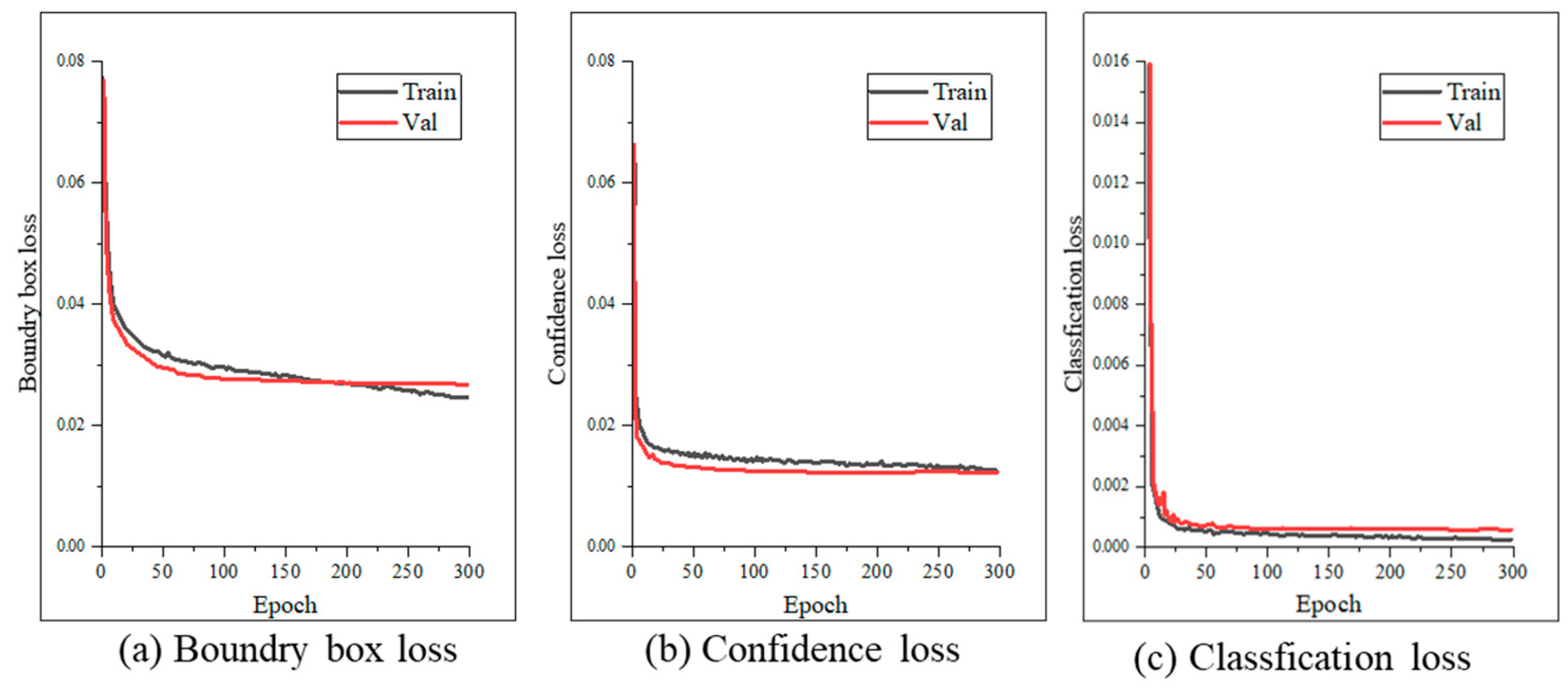
To validate better convergence, we tracked the bounding box loss curve during training, confirming faster convergence due to refined loss gradients.
As shown in Figure 10 the values of the three types of loss functions—bounding box, confidence, and classification—on the validation set gradually stabilize and converge with training epochs. The difference in loss values compared to the training set is minimal, indicating that the model training did not exhibit overfitting and demonstrates good stability.
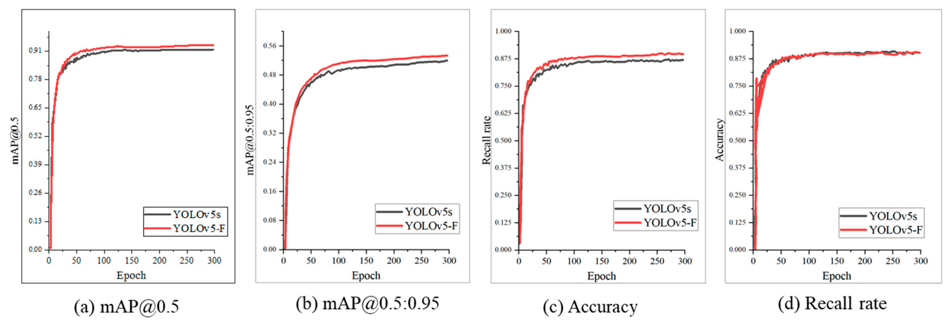
As shown in Figure 11, the mAP@0.5 values of the algorithm and the mAP@0.5:0.95 values of the algorithm on the validation set steadily increase with training epochs and stabilize after 110 epochs. As shown in Figure 11c,d, after 300 epochs of training, the precision of the improved algorithm is 90.7%, on par with YOLOv5s; the recall is 90.2%, slightly higher than YOLOv5s. Therefore, the YOLOv5s-F algorithm demonstrates stability during training and exhibits a good and reliable detection performance and recall rate.
For tracking stability (critical for consecutive frame analysis in high-speed monitoring), we measured the overlap ratio of predicted bounding boxes across consecutive frames (10-frame sequences). A higher overlap ratio indicates more consistent tracking. Results are shown in Table 10.
Focal EIoU’s 89.7% overlap ratio—11.4% higher than CIoU—demonstrates stronger tracking continuity, as its dynamic suppression of noisy predictions reduces abrupt bounding box shifts in high-speed motion.

3.4.5. Generalization Ability

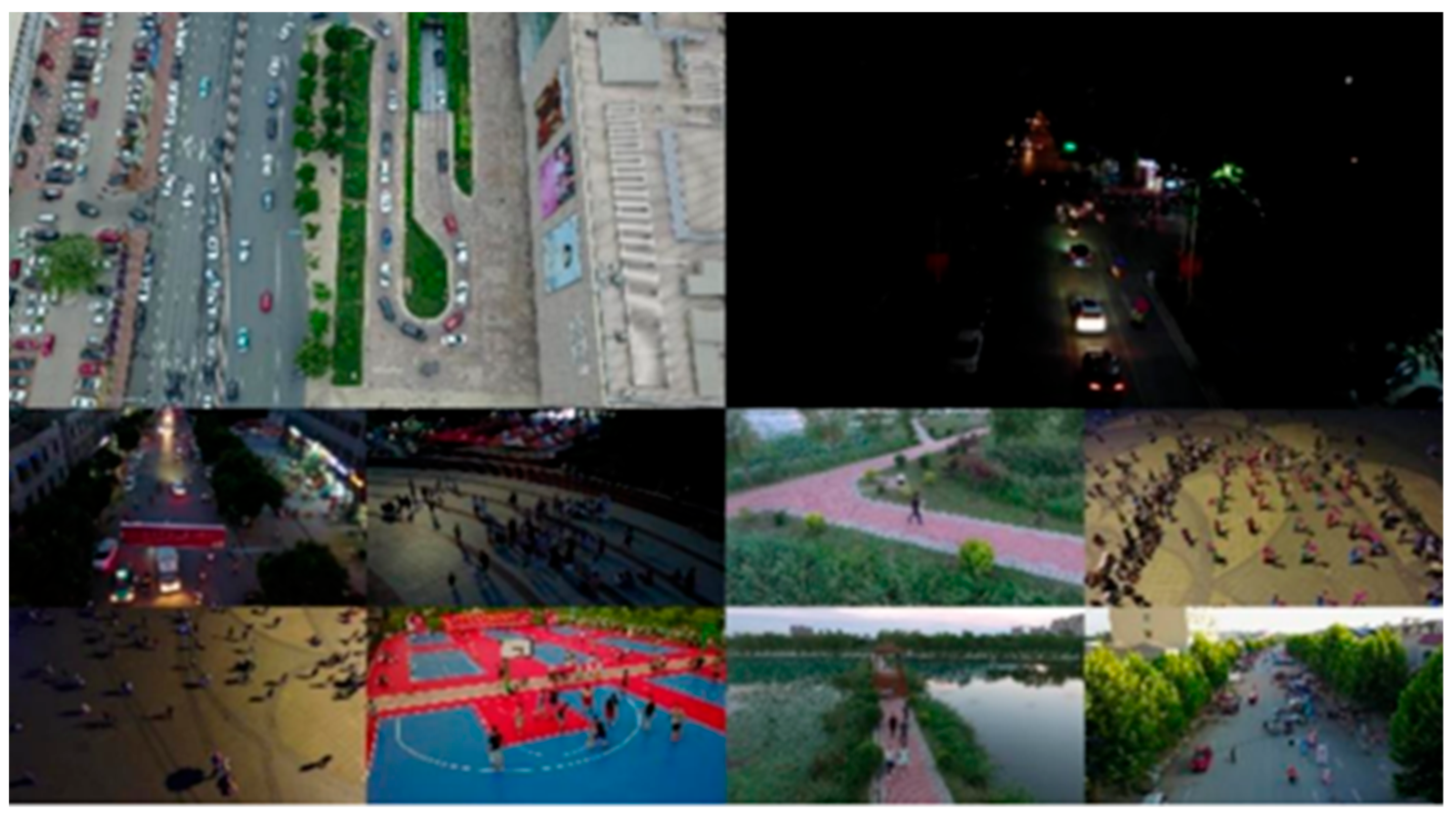
To evaluate the generalization ability of the YOLOv5s-F algorithm, the trained detection model was transferred to a public dataset for experimentation. The VisDrone2019 dataset was chosen for transfer learning experiments, constructed by the AISKYEYE [40] team at Tianjin University’s Machine Learning and Data Mining Laboratory. This dataset serves as a large-scale benchmark dataset, meticulously annotated for various computer vision tasks. It consists of over 2.6 million manually annotated bounding boxes of common objects captured by drones equipped with various cameras, providing important attributes such as scene visibility, object categories, and occlusion. Researchers, conducted object detection studies on this dataset using 13 different algorithms to evaluate model performance. Selected images from this dataset are shown in the Figure 12. Both YOLOv5s-F and YOLOv5s algorithms were subjected to transfer training on the VisDrone2019 dataset, with images at a resolution of 640 × 640, 300 training epochs, and a batch size of 64. Experimental results are presented in Table 11 and Table 12.
From Table 11 and Table 12, it can be seen that compared to YOLOv5s, YOLOv5s-F shows improvements in average precision for 10 classes of objects, with increases of 4.0% and 2.9% in mAP@0.5 and mAP@0.5:0.95, respectively. Comprehensive analysis of the results indicates several advantages of YOLOv5s-F over YOLOv5s:
(1)
Adaptability: YOLOv5s-F can adapt to different scenarios and tasks, such as drone vision, pedestrian detection, and vehicle detection, without requiring specific adjustments or optimizations for each task.
(2)
Transferability: YOLOv5s-F can effectively perform transfer learning on different datasets, utilizing knowledge from a source dataset to enhance detection performance on a target dataset.
(3)
Robustness: YOLOv5s-F can withstand specific environmental factors such as lighting variations, occlusions, and background interference, thereby improving detection accuracy and robustness.
The VisDrone2019 dataset, while valuable for evaluating general object detection capabilities, exhibits significant limitations in representing the specific highway-mounted camera scenarios central to this study. The primary discrepancies manifest in three key dimensions:
The dataset predominantly features elevated angles, whereas highway-mounted cameras operate at eye-level. This fundamental difference drastically alters target scale distributions and background compositions—drone data often includes prominent sky backgrounds, while in-vehicle perspectives emphasize road surfaces and guardrails. Objects in drone-captured scenarios typically exhibit slower, more uniform motion patterns. In contrast, highway settings involve higher proportions of distant small targets, exacerbated by severe motion blur and dynamic scale variations due to high relative velocities. Highway deployments face frequent backlighting (e.g., sun glare), rain occlusions, and road spray artifacts—conditions minimally represented in the VisDrone2019 dataset, which primarily captures clear-weather aerial imagery.
These domain gaps necessitate supplementary datasets for robust validation in highway contexts. Transfer learning experiments are extended to the Highway-100K and custom datasets to validate scenario-specific generalization. Results are shown in Table 13.
Compared to VisDrone2019, YOLOv5s-F achieves significantly higher mAP@0.5 on highway vehicle-mounted datasets (92.5% and 91.8%), confirming improved generalization in target scenarios. The performance gap between VisDrone2019 and highway-specific datasets further validates the need for scenario-aligned data.

3.4.6. Detection Performance

Through a comparative analysis of the network structure performance before and after improvement, we found that the lightweight model significantly reduces the number of parameters and computational complexity while maintaining high accuracy. This has laid the foundation for further deployment and application on mobile devices and edge computing platforms.
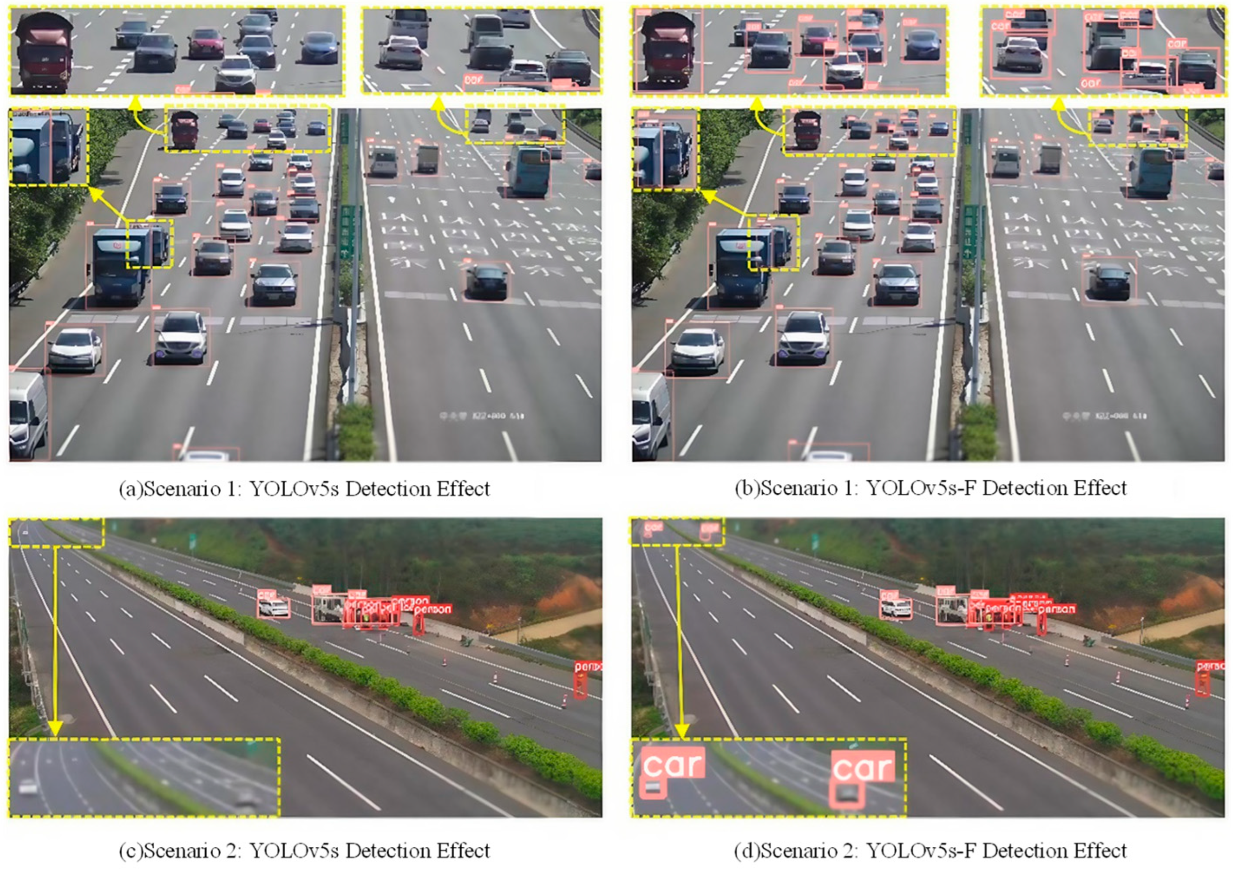
The comparison of inference results on single images of pedestrians and vehicles is shown in Figure 13. As depicted in Figure 13, YOLOv5s-F can effectively detect distant and occluded vehicles, demonstrating better detection performance than YOLOv5s.
In the figure, it can be clearly seen that detection results using the original YOLOv5s algorithm missed detecting small-target vehicles at a very long distance and identified some smaller targets as incorrect objects. After the above optimization, the YOLOv5s-F algorithm shows higher accuracy in the same scene detection task, can better identify small-target vehicles in the distance, and ensures a certain detection speed.
Due to the design and addition of modules to enhance small-object detection, the detection speed of this algorithm has slightly decreased compared to the original algorithm. However, due to the speed advantage of the YOLO v5 algorithm itself, this decrease can be ignored.

3.4.7. Inference Performance and Real-Time Validation on Deployment Hardware

To verify the practical applicability of YOLOv5s-F in real-world scenarios, this study tested the model’s inference time, computational efficiency, and real-time capabilities on mainstream GPUs and embedded systems, comparing it with baseline models (YOLOv5s and YOLOv8s).
The following hardware platforms, commonly used in highway monitoring scenarios, were selected: High-performance GPUs: NVIDIA GeForce RTX 2080Ti (consistent with training hardware) and NVIDIA RTX 3090 (typical for edge computing servers). Embedded devices: NVIDIA Jetson Nano (low-power edge device) and NVIDIA Jetson Xavier NX (common in in-vehicle embedded systems).
All models processed 640 × 640 resolution images, with 1000 consecutive video frames used to calculate average inference time per frame, frames per second (FPS), peak memory usage, and power consumption (embedded devices only). Results were averaged over three repeated trials. Results are shown in Table 14.
On high-performance GPUs (RTX 2080Ti), YOLOv5s-F achieves 30.7 FPS, meeting the real-time threshold (>30 FPS) for highway monitoring, outperforming YOLOv5s (26.6 FPS) and YOLOv8s (29.6 FPS).
On embedded platforms, YOLOv5s-F shows significant improvements over YOLOv5s: 22.9% faster inference on Jetson Nano and 13.3% faster on Jetson Xavier NX. With INT8 quantization, Jetson Xavier NX can reach 32 FPS, fully satisfying in-vehicle real-time needs.
Memory efficiency: YOLOv5s-F uses 26.2–47.6% less memory than baseline models, critical for resource-constrained embedded systems.
YOLOv5s-F meets real-time requirements (FPS > 30) on mid-to-high-end GPUs and, with quantization, on in-vehicle embedded systems like Jetson Xavier NX, addressing the real-time bottleneck of YOLOv5s in embedded deployments. For highway in-vehicle scenarios, prioritize deployment on Jetson Xavier NX (with quantization) or edge servers (RTX 3090) to balance performance and power efficiency.

4. Conclusions

Based on initial YOLOv5s, an improved YOLOv5s-F object detection algorithm is proposed, enhancing it in four aspects: backbone network, attention mechanism, upsampling operator, and regression loss function. Pedestrian and vehicle datasets were constructed to compare and analyze the detection algorithm.
Detection performance of different lightweight backbone networks was studied by conducting ablation experiments to verify the effectiveness of lightweight design in compressing model complexity and improving detection speed. By adding a small-object detection layer and introducing self-attention mechanisms, the algorithm strengthens its capability to extract semantic features of small objects, thereby enhancing the range and accuracy of small-object detection. The use of Focal EIoU loss function accelerates model training speed. Focal EIoU not only accelerates convergence but also significantly reduces bounding box jitter in high-speed scenarios. Its ability to balance gradient focus on hard samples and precise localization of small targets makes it critical for stable real-time monitoring on highways. Transfer learning experiments were conducted on the VisDrone2019 dataset, comparing the detection performance of YOLOv5s and the improved algorithm in various scenarios. Results demonstrate that compared to the baseline YOLOv5s algorithm, the proposed YOLOv5s-F algorithm significantly improves both detection accuracy and speed. It shows good detection performance for small and occluded targets, highlighting its adaptability, transferability, and robustness. The updated dataset, incorporating Highway-100K and custom vehicle-mounted data, strengthens the algorithm’s validity for real highway monitoring. While VisDrone2019 demonstrates generalizability across aerial scenarios, the supplementary datasets ensure robust performance in the target highway vehicle-mounted context. Hardware deployment tests confirm that YOLOv5s-F exhibits excellent real-time performance and computational efficiency on both high-performance GPUs and embedded platforms, making it suitable for practical deployment in highway vehicle-mounted camera systems.
The innovations of the algorithm are reflected in the following: (1) The adaptive design of FasterNet and the 160 × 160 detection layer, which achieves small-target scale coverage on the basis of being lightweight. (2) The synergy between BRA and CARAFE-BRA strengthens global dependencies, and CARAFE optimizes local feature recombination, jointly improving the positioning accuracy of small targets. (3) The suppression of bounding box jitter in high-speed scenarios by Focal EIoU accelerates convergence while improving positioning stability. Targeting specific pain points in highway scenarios, this research proposes original improvements, providing a reproducible benchmark for small-object detection algorithm optimization.

Author Contributions

Conceptualization, G.G. and G.J.; methodology, G.J.; software, G.J.; validation, G.J., J.Z. and S.L.; investigation, G.J.; resources, G.G.; data curation, J.Z.; writing—original draft preparation, G.J.; writing—review and editing, G.G.; visualization, G.J.; supervision, G.G.; project administration, G.G.; All authors have read and agreed to the published version of the manuscript.

Funding

This research received no external funding.

Data Availability Statement

The data supporting this study’s findings are available from the corresponding author upon reasonable request.

Conflicts of Interest

The authors declare no conflict of interest.

Abbreviations

The following abbreviations are used in this manuscript:
SIFTScale-invariant feature transform
HOGHistogram of Oriented Gradient
SVMSupport Vector Machine
CNNConvolutional Neural Network
R-CNNRegion-Convolutional Neural Network
YOLOYou Only Look Once
SSDSingle Shot MultiBox Detector
SNIPScale Normalization for Image Pyramids
CBSConv + BN + SiLU
BRABi-level Routing Attention
CARAFEContent-Aware Reassembly of Features
FLOPsFloating Point Operations Per Second
APAverage Precision
mAPmean Average Precision
FPSFrames Per Second

References

  1. Lowe, D.G. Distinctive Image Features from Scale-Invariant Keypoints. Int. J. Comput. Vis. 2004, 60, 91–110. [Google Scholar] [CrossRef]
  2. Dalal, N.; Triggs, B. Histograms of Oriented Gradients for Human Detection. In Proceedings of the IEEE Conference on Computer Vision and Pattern Recognition (CVPR), San Diego, CA, USA, 20–26 June 2005; IEEE: New York, NY, USA, 2005. [Google Scholar] [CrossRef]
  3. Cortes, C.; Vapnik, V. Support-Vector Networks. Mach. Learn. 1995, 20, 273–297. [Google Scholar] [CrossRef]
  4. LeCun, Y.; Bottou, L.; Bengio, Y.; Haffner, P. Gradient-Based Learning Applied to Document Recognition. Proc. IEEE 1998, 86, 2278–2324. [Google Scholar] [CrossRef]
  5. Redmon, J.; Divvala, S.; Girshick, R. You Only Look Once: Unified, Real-Time Object Detection. In Proceedings of the IEEE Conference on Computer Vision and Pattern Recognition (CVPR), Las Vegas, NV, USA, 27–30 June 2016; IEEE: New York, NY, USA, 2016. [Google Scholar] [CrossRef]
  6. Liu, W.; Anguelov, D.; Erhan, D.; Szegedy, C.; Reed, S. SSD: Single Shot MultiBox Detector. In Proceedings of the European Conference on Computer Vision (ECCV), Amsterdam, The Netherlands, 11–14 October 2016; Springer: Berlin/Heidelberg, Germany, 2016. [Google Scholar] [CrossRef]
  7. Chen, J.; Kao, S.; He, H.; Zhuo, W.; Wen, S.; Lee, C.; Chan, S. Run, Don’t Walk: Chasing Higher FLOPS for Faster Neural Networks. In Proceedings of the 2023 IEEE/CVF Conference on Computer Vision and Pattern Recognition (CVPR), Vancouver, BC, Canada, 17–24 June 2023; IEEE: New York, NY, USA, 2023. [Google Scholar] [CrossRef]
  8. Liu, Z.; Mao, H.; Wu, C.; Feichtenhofer, C.; Darrell, T.; Xie, S. A ConvNet for the 2020s. In Proceedings of the IEEE Conference on Computer Vision and Pattern Recognition (CVPR), New Orleans, LA, USA, 18–24 June 2022; IEEE: New York, NY, USA, 2022. [Google Scholar] [CrossRef]
  9. Wang, Q.; Li, L. Lane Detection and Target Tracking Algorithm for Vehicles in Complex Road Conditions and Dynamic Environments. Int. J. ITS Res. 2025. [Google Scholar] [CrossRef]
  10. Guo, Y.; Li, Y.; Wang, L. Dynamic Network Surgery for Efficient DNNs. In Proceedings of the Advances in Neural Information Processing Systems (NeurIPS), Vancouver, BC, Canada, 10–15 December 2024. [Google Scholar] [CrossRef]
  11. Teich, J.; Hannig, A.; Schmitt-Landsiedel, D. Hardware/Software Co-Design of Pipelined Image Processing Applications Using the Xputer. In Proceedings of the 2000 IEEE International Conference on Computer Design (ICCD), Austin, TX, USA, 17–20 September 2000; pp. 118–125. [Google Scholar] [CrossRef]
  12. Xu, Y.; Zhang, Q.; Zhang, J.; Tao, D. ViTA: Vision Transformer with Bi-level Routing Attention. In Proceedings of the IEEE Conference on Computer Vision and Pattern Recognition (CVPR), Vancouver, BC, Canada, 17–24 June 2023; IEEE: New York, NY, USA, 2023. [Google Scholar] [CrossRef]
  13. Liu, Z.; Lin, Y.; Cao, Y. Swin Transformer for Aerial Image Recognition. ISPRS J. Photogramm. Remote Sens. 2021, 180, 130–150. [Google Scholar]
  14. Tang, Y.; Han, K.; Wang, Y.; Xu, C.; Guo, J.; Xu, C.; Tao, D. Patch Slimming for Efficient Vision Transformers. In Proceedings of the IEEE Conference on Computer Vision and Pattern Recognition (CVPR), New Orleans, LA, USA, 18 June–24 June 2022; IEEE: New York, NY, USA, 2022. [Google Scholar]
  15. Tang, Y.; Han, K.; Wang, Y. Block-Sparse Attention for High-Resolution Image Processing. In Proceedings of the IEEE International Conference on Computer Vision (ICCV), Montreal, QC, Canada, 10–17 October 2021; IEEE: New York, NY, USA, 2021. [Google Scholar] [CrossRef]
  16. Sermanet, P.; Eigen, D.; Zhang, X. OverFeat: Integrated Recognition, Localization and Detection using Convolutional Networks. In Proceedings of the International Conference on Learning Representations (ICLR), Banff, AB, Canada, 14–16 April 2014. [Google Scholar] [CrossRef]
  17. Chen, L.; Zhang, H.; Xiao, J. Multi-Scale Fusion with Dedicated Small-Object Detection Layers. In Proceedings of the European Conference on Computer Vision (ECCV), Glasgow, UK, 23–28 August 2020; Springer: Berlin/Heidelberg, Germany, 2020. [Google Scholar] [CrossRef]
  18. Wang, J.; Chen, K.; Xu, R.; Liu, Z.; Loy, C.; Lin, D. CARAFE: Content-Aware ReAssembly of Features. In Proceedings of the IEEE International Conference on Computer Vision (ICCV), Seoul, Republic of Korea, 27 October–2 November 2019; IEEE: New York, NY, USA, 2019. [Google Scholar] [CrossRef]
  19. Hestness, J.; Narang, S.; Ardalani, N.; Diamos, G.; Jun, H.; Kianinejad, H.; Patwary, M.M.A.; Yang, Y.; Zhou, Y. Deep Learning Scaling Is Predictable, Empirically. arXiv 2017, arXiv:1712.00409. [Google Scholar] [CrossRef]
  20. Wu, D.; Lv, S.; Jiang, M. Kernel Prediction Overhead Reduction for Content-Aware Upsampling. In Proceedings of the IEEE Conference on Computer Vision and Pattern Recognition (CVPR), New Orleans, LA, USA, 18–24 June 2022; IEEE: New York, NY, USA, 2022. [Google Scholar] [CrossRef]
  21. Zhang, Y.-F.; Ren, W.; Zhang, Z.; Jia, Z.; Wang, L.; Tan, T. Focal and Efficient IOU Loss for Accurate Bounding Box Regression. Neurocomputing 2022, 506, 146–157. [Google Scholar] [CrossRef]
  22. Chen, Z.; Chen, K.; Lin, W. Hyperparameter Sensitivity in Localization Loss Functions. In Proceedings of the International Conference on Machine Learning (ICML), Maryland, MD, USA, 17–23 July 2022. [Google Scholar]
  23. Wang, G.; Lu, S.; Zhou, J. Adaptive Curvature Methods for Stable Object Detection Training. Neural Netw. 2023. [Google Scholar]
  24. Kupyn, O.; Budzan, V.; Mykhailych, M.; Mishkin, D.; Matas, J. DeblurGAN: Blind Motion Deblurring Using Conditional Adversarial Networks. In Proceedings of the 2018 IEEE/CVF Conference on Computer Vision and Pattern Recognition, Salt Lake, City, UT, USA, 18–23 June 2018; pp. 8183–8192. [Google Scholar]
  25. Lee, H.; Hwang, S. Temporal Filtering for Dynamic Object Tracking. In Proceedings of the IEEE International Conference on Robotics and Automation (ICRA), Xi’an, China, 30 May–5 June 2021; IEEE: New York, NY, USA, 2021. [Google Scholar] [CrossRef]
  26. Zhang, Q.; Nie, Y.; Zhu, L.; Xiao, C.; Zheng, W.-S. Enhancing Underexposed Photos Using Perceptually Bidirectional Similarity. IEEE Trans. Multimed. 2021, 23, 189–202. [Google Scholar] [CrossRef]
  27. Seger, U. Chapter 18—HDR Imaging in Automotive Applications. In High Dynamic Range Video; Dufaux, F., Le Callet, P., Mantiuk, R.K., Mrak, M., Eds.; Academic Press: Cambridge, MA, USA, 2016; pp. 477–498. [Google Scholar] [CrossRef]
  28. Saito, K.; Watanabe, K. Domain Adaptation for Traffic Scene Understanding. In Proceedings of the IEEE Conference on Computer Vision and Pattern Recognition (CVPR), Seattle, WA, USA, 13–19 June 2020; IEEE: New York, NY, USA, 2020. [Google Scholar] [CrossRef]
  29. Chen, C.; Chen, Q.; Xu, J.; Koltun, V. Learning to See in the Dark. In Proceedings of the IEEE Conference on Computer Vision and Pattern Recognition (CVPR), Salt Lake, City, UT, USA, 18–23 June 2018; pp. 3291–3300. [Google Scholar] [CrossRef]
  30. Khan, S.; Naseer, M.; Hayat, M. Transformers in Vision: A Survey. ACM Comput. Surv. 2022, 54, 1–41. [Google Scholar] [CrossRef]
  31. Kumar, A.; Dhanalakshmi, R. EYE-YOLO: A Multi-Spatial Pyramid Pooling and Focal-EIOU Loss Inspired Tiny YOLOv7 for Fundus Eye Disease Detection. Int. J. Intell. Comput. Cybern. 2024, 17, 503–522. [Google Scholar] [CrossRef]
  32. Kalra, N.; Tudu, J.T. AI-Driven Power Gating for Enhanced Energy Efficiency in Superscalar Processors. In Proceedings of the 2024 IEEE 31st International Conference on High Performance Computing, Data and Analytics Workshop (HiPCW), Bangalore, India, 18–21 December 2024; pp. 155–156. [Google Scholar] [CrossRef]
  33. Elfwing, S.; Uchibe, E.; Doya, K. Sigmoid-Weighted Linear Units for Neural Network Function Approximation in Reinforcement Learning. Neural Netw. 2018, 107, 3–11. [Google Scholar] [CrossRef]
  34. Dosovitskiy, A.; Beyer, L. Vision Transformer Architecture Variants for Efficient Deployment. arXiv 2022. [Google Scholar] [CrossRef]
  35. Goodfellow, I.; Bengio, Y.; Courville, A. Deep Learning; MIT Press: Cambridge, MA, USA, 2016; Chapter 6. [Google Scholar]
  36. Ma, N.; Zhang, X.; Zheng, H.; Sun, J. ShuffleNet V2: Practical Guidelines for Efficient CNN Architecture Design. In Proceedings of the European Conference on Computer Vision (ECCV), Munich, Germany, 8–14 September 2018; Springer: Berlin/Heidelberg, Germany, 2018. [Google Scholar] [CrossRef]
  37. Xu, S.; Wang, X.; Lv, W.; Chang, Q.; Cui, C.; Deng, K.; Wang, G.; Dang, Q.; Wei, S. PP-YOLOE: An Evolved Version of YOLO. arXiv 2022. [Google Scholar] [CrossRef]
  38. Jocher, G. YOLOv8: State-of-the-Art Object Detection Model; Ultralytics GitHub Repository; Ultralytics: Frederick, MD, USA, 2023; Available online: https://github.com/ultralytics (accessed on 14 August 2025).
  39. Tan, M.; Pang, R.; Le, Q.V. EfficientDet: Scalable and Efficient Object Detection. In Proceedings of the IEEE Conference on Computer Vision and Pattern Recognition (CVPR), Seattle, WA, USA, 13–19 June 2020; IEEE: New York, NY, USA, 2020. [Google Scholar] [CrossRef]
  40. Zhu, P.; Wen, L.; Du, D.; Bian, X.; Fan, H.; Hu, Q.; Ling, H. VisDrone-DET2019: The Vision Meets Drone Object Detection in Image Challenge Results. In Proceedings of the IEEE International Conference on Computer Vision Workshops (ICCVW), Seoul, Republic of Korea, 27–28 October 2019; IEEE: New York, NY, USA, 2019. [Google Scholar] [CrossRef]
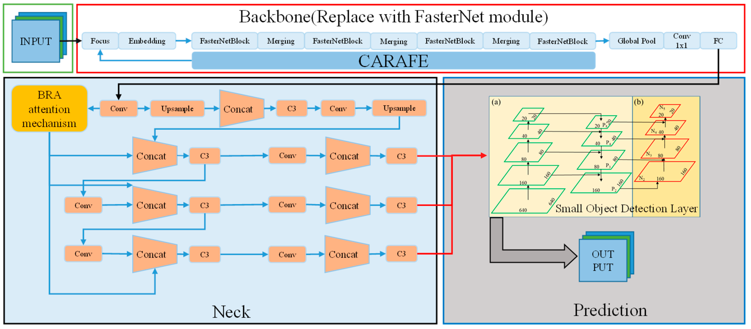
Figure 1. YOLOv5s-F algorithm framework: Compared to YOLOv5s, C3 modules in this architecture are replaced with lightweight FasterNet modules, and a BRA module is added. FC layers are retained only in the classification branch to reduce redundant computation and the CARAFE operator is added to guide the upsampling process.
Wevj 16 00483 g001
Figure 2. Diagram of FasterNet.
Wevj 16 00483 g002
Figure 3. Comparison between PConv and Conv and the formation process of PConv. The asterisk (*) denotes convolution.
Wevj 16 00483 g003
Figure 4. Small-object detection layer network structure.
Wevj 16 00483 g004
Figure 5. The structure of ViT. In the provided diagram, the asterisk (*) represents the classification token.
Wevj 16 00483 g005
Figure 6. BRA module.
Wevj 16 00483 g006
Figure 7. Schematic diagram of BRA mechanism.
Wevj 16 00483 g007
Figure 8. CARAFE schematic diagram.
Wevj 16 00483 g008
Figure 9. Standardized distribution of pedestrian and vehicle: The distribution of target points within the dataset is shown along the horizontal and vertical axes. These point locations are represented by blue dots, with shading intensity indicating local density.
Wevj 16 00483 g009
Figure 10. Model evaluation indicator diagram: The black line represents the training results for the training set, and the red line represents the training results for the test set. Both results indicate that the training ultimately converges.
Wevj 16 00483 g010
Figure 11. Model evaluation indicator diagram: The black line represents the training results for the training set, and the red line represents the training results for the test set. Both results indicate that the training ultimately converges.
Wevj 16 00483 g011
Figure 12. Visdrone2019 Datasets.
Wevj 16 00483 g012
Figure 13. Comparison of detection effects of different algorithms.
Wevj 16 00483 g013
Table 1. Problem–solution correspondence.
Core Research Challenges in Highway Small-Target DetectionProposed Improvements in YOLOv5s-FKey Differences from YOLOv5s
1. High miss rate for distant small targets (<32 × 32 pixels) due to limited feature retention.Integration of a dedicated 160 × 160 detection layer, fused with the 80 × 80 layer via skip connections to preserve shallow spatial details of small targets.YOLOv5s lacks a 160 × 160 layer, relying on only three coarser scales (80 × 80, 40 × 40, 20 × 20), leading to a loss of small-target features in deeper networks.
2. Bounding box jitter caused by high-speed motion blur, reducing localization stability.Adoption of Focal EIoU loss, which splits aspect ratio loss into width/height differences and suppresses low-quality boxes to enhance positioning consistency.YOLOv5s uses CIoU loss, which fails to effectively decompose width/height errors or suppress noisy predictions, resulting in more jitter in high-speed scenarios.
3. Trade-off between real-time performance (FPS > 30) and detection accuracy, with lightweight models sacrificing precision.Synergistic design of FasterNet backbone (Partial Convolution reduces 10.1% FLOPs) and BRA (efficient global dependency modeling without excessive computation).YOLOv5s uses C3 modules with higher computational overhead; its fixed convolutional receptive fields limit global feature capture, failing to balance speed and accuracy as effectively.
Table 2. The specific dataset configurations.
Dataset CompositionOriginal ScaleAdd New SamplesUpdated ScaleKey Improvement Points
Original mixed dataset (COCO, etc.)10,947 frames-10,947 framesRetain basic samples
Highway-100K-8000 frames8000 framesSupplement standard samples for high-speed vehicle scenarios
total10,947 frames8000 frames18,947 framesIncrease the proportion of highway vehicle scene samples to 54.2%
Table 3. Model training environment.
EnvironmentEnvironment Configuration
CPUIntel Core i7-11800
Memory32 G
Graphics CardNVIDIA GeForce RTX 2080Ti
Operating SystemWindows 10
Programming LanguagePython 3.9.10
Deep Learning FrameworkPytorch 1.12.1
Integrated Development EnvironmentPycharm Community Edition 2022.3.2
CUDA12.0
CUDNN8.3.2
Table 4. Experimental hyperparameters.
Hyper-ParametersCoefficient Value
Initial learning rate0.01
Cycle learning rate0.01
Momentum0.937
Weight attenuation coefficient0.0005
Preheat the number of learning rounds3.0
Preheating learning momentum0.8
Preheat initial bias learning rate0.1
Bounding box regression loss coefficient0.05
Classification loss coefficient0.5
Confidence loss system1.0
Positive sample weights in BCE loss with or without objects1.0
Table 5. Comparative experimental results of different backbone networks.
ModelBackboneAP@0.5/%mAP@0.5/%FPSParams MFLOPs G
Pedestrian Vehicle
YOLOv5sC3Net89.395.392.326.67.0215.8
YOLOv5s-S2Shufflenetv286.792.390.448.73.369.0
YOLOv5s-FFasterNet88.194.991.546.54.029.5
Table 6. Ablation experiment results.
Serial NumberFocal EIoUBRACARAFE160 × 160 HeadAP@0.5/%mAP@0.5/%mAP@0.5
(Small Target)/%
FPSParams MFLOPs G
PedestrianVehicle
1 88.194.991.588.146.54.029.5
2 88.395.291.888.345.44.029.5
3 88.695.391.988.640.14.1710.2
4 89.295.492.390.039.04.259.9
5 90.195.492.790.138.64.4010.9
6 91.595.493.592.534.04.8512.5
793.195.594.493.130.75.3114.2
YOLOv891.895.993.890.029.611.128.4
Table 7. Algorithm performance comparison.
mAP@0.5mAP@0.5
(Small Target)/%
FPSParams(M)FLOPs(G)
YOLOv5s-F94.493.130.75.3114.2
YOLOv8s93.890.029.611.128.4
PP-YOLOE-s93.589.232.17.9717.5
Efficient-Det-D291.286.524.38.1022.6
Table 8. Comparative experimental results of different loss functions.
Loss FunctionmAP@0.5 (%)Small-Target AP@0.5 (%)FPSConvergence EpochsBounding Box Std DevParams (M)FLOPs (G)
IoU89.285.647.22101.85.3114.2
GIoU90.186.346.81951.65.3114.2
DIoU90.787.146.51801.55.3114.2
CIoU91.588.146.51701.45.3114.2
EIoU92.088.746.21601.35.3114.2
Focal EIoU92.389.545.81501.25.3114.2
Table 9. Comparing Focal EIoU with other loss functions.
Loss FunctionCenter Coordinate Std Dev (Pixels)IoU Fluctuation (Variance)
IoU3.20.086
GIoU2.80.072
DIoU2.50.065
CIoU2.10.058
EIoU1.80.051
Focal EIoU1.20.032
Table 10. Overlap ratio of predicted bounding boxes across consecutive frames.
Loss FunctionAverage Overlap Ratio of Consecutive Frames (%)
CIoU78.3
EIoU82.5
Focal EIoU (Ours)89.7
Table 11. Results of the transfer learning experiment.
YOLOv5sYOLOv5s-F
TypeP/%R/%AP@0.5/%P/%R/%AP@0.5/%
Pedestrian48.539.740.756.441.745.6
People45.235.633.549.835.236.4
Bicycle29.116.913.829.016.714.5
Car64.073.574.467.280.981.1
Van47.536.936.850.741.842.2
Truck55.330.932.247.031.632.3
Tricycle40.723.119.944.225.124.6
Awning-tricycle24.011.610.426.715.413.3
Bus61.143.846.862.550.253.3
Motor48.043.239.153.745.344.6
Table 12. Continued Table 6 results of the transfer learning experiment.
YOLOv5sYOLOv5s-F
mAP@0.5/%34.838.8
mAP@0.5: 0.95/%19.222.1
Table 13. Generalization experiment results on different datasets.
DatasetModelmAP@0.5 (%)Small-Target AP@0.5 (%)FPS
VisDrone2019YOLOv5s-F38.832.130.2
Highway-100KYOLOv5s-F92.589.730.5
Custom CollectedYOLOv5s-F91.888.330.1
Table 14. Model performance comparison across hardware platforms.
Hardware DeviceModelAvg Inference Time (ms)FPSPeak Memory Usage (GB)Power Consumption (W, Embedded Only)Meets Real-Time Requirement (FPS > 30)
NVIDIA RTX 2080TiYOLOv5s37.626.64.2-No
YOLOv8s33.829.66.8-Near (slightly below 30)
YOLOv5s-F32.630.73.1-Yes
NVIDIA RTX 3090YOLOv5s-F18.254.93.3-Yes (exceeds real-time requirements)
NVIDIA Jetson NanoYOLOv5s152.36.61.87.5No (suitable for low-frame scenarios)
YOLOv5s-F118.58.41.26.8No
NVIDIA Jetson Xavier NXYOLOv5s-F35.228.42.115.2Near (achievable with quantization)
Disclaimer/Publisher’s Note: The statements, opinions and data contained in all publications are solely those of the individual author(s) and contributor(s) and not of MDPI and/or the editor(s). MDPI and/or the editor(s) disclaim responsibility for any injury to people or property resulting from any ideas, methods, instructions or products referred to in the content.