Research on Trajectory Tracking Control of Driverless Electric Formula Racing Cars Based on Prescribed Performance and Fuzzy Logic Systems

Abstract

Driverless electric formula racing cars are affected by nonlinear vehicle characteristics, perturbations, and parameter uncertainties during races, which can cause problems such as low accuracy and instability in trajectory tracking. Aiming to address such problems, this paper proposes a control method combining a prescribed performance control with adaptive backstepping fuzzy control (PPC-ABFC) to solve the aforementioned issues and improve the trajectory tracking accuracy and stability of racing cars. This control method is achieved by constructing a combined error model and confining the error within a prescribed performance function. The nonlinear terms, disturbances, and unknown parameters of the model are approximated by a fuzzy logic system (FLS). An adaptive parameter update law is designed to update the learning parameters in real time. The virtual control law and the real control law were designed by using the backstepping method. The stability of the PPC-ABFC closed-loop system was rigorously proved by applying the Lyapunov stability theory. Finally, simulations were conducted to compare the proposed PPC-ABFC method with other algorithms at different speeds. The results demonstrated that the PPC-ABFC method effectively enhances the trajectory tracking performance of driverless electric formula racing cars.

1. Introduction

With the rapid development of science and technology, human society has entered the era of intelligence. With the rapid development of artificial intelligence and the automobile industry, driverless technology has gradually become the focus of the industry [1,2,3]. Driverless electric formula racing competitions closely follow the development of the automotive industry, among which high-speed trajectory tracking race events are the most challenging for driverless driving technology. The environment sensing system obtains road information [4], the path decision and planning system [5] designs the running trajectory of the racing car, and the trajectory tracking system carries out the lateral and longitudinal control of the racing car according to the designed trajectory, with lateral control being a key part of the motion of driverless racing car during competitions [6]. Due to the fact that the vehicle system is a highly complex, nonlinear, and strongly coupled system, precise control of lateral movement still poses certain challenges for racing cars during high-speed operation [7]. This paper conducts research on the lateral control of driverless electric formula racing cars.

In the field of driverless vehicle control, scholars at home and abroad have proposed a variety of control algorithms, such as model predictive control (MPC) [8,9], linear optimal quadratic control (LQR) [10,11], proportion integral derivative (PID) [12], sliding mode control (SMC) [13,14], fuzzy control [15,16], neural network control [17], feedback–feedforward control, and so on. Recently, many scholars have used MPC for trajectory tracking control of vehicles and combined it with other algorithms to improve the control accuracy. Duanfeng Chu et al. [18] proposed a combined MPC and PID feedback control method, which can eliminate the errors caused by simplifying the vehicle model in the traditional MPC. Tian Tian et al. [19] proposed a MPC trajectory tracking control method based on game theory, which introduces the trajectory tracking accuracy and stability as a time-varying interactive game mechanism, establishes a game payoff matrix, and determines the weights of each subject to find the optimal control strategy in the MPC. Dele Meng et al. [20] proposed a fast iterative MPC (FI-MPC) equation, which integrates the unmodeled nonlinear dynamics of the vehicle and tires into a linear system framework to mitigate the mismatch between linear and high-fidelity nonlinear dynamics models to achieve the optimal iterative control scheme. However, MPC has some shortcomings; for example, it requires strong real-time computational capability on the hardware side and relies on a high-precision vehicle model, but as the vehicle is a nonlinear system with uncertain state parameters, it is difficult to establish an accurate vehicle model.

Later, in response to issues such as nonlinearity, a large number of scholars conducted research. The adaptive backstepping method [21], prescribed performance control (PPC) [22], and reinforcement learning technologies have been widely applied. Wang Aojie et al. [23] proposed a fixed-time global sliding mode control with prescribed performance, which solved the trajectory tracking problem of robots with uncertain models, limited the system error within the performance boundary, and improved the global robustness and convergence performance. Yang Pu et al. [24] proposed a method based on the prescribed performance function and non-singular approximate fixed-time terminal sliding mode, which solved the problems of parameter uncertainty during the trajectory tracking of robot manipulators, and the prescribed performance function provided higher steady-state accuracy. It can be seen that the PPC has achieved satisfactory results in different industrial fields. The main idea of designing the controller using the backstepping control method is to decompose the complex nonlinear system into several subsystems, then construct error variables, design virtual control laws for each subsystem, and finally design the actual controller and prove the global stability of the entire closed-loop system. Binzhen Liu et al. [25] proposed a method based on finite-time convergence, combined with the command filtering backstepping method to ensure the convergence performance, introduced a compensation mechanism to reduce the filtering error, and solved the tracking problem of flexible multi-joint robotic arms. However, the backstepping method did not solve the problems of the nonlinear terms and disturbances in the model.

To address the aforementioned issues, many scholars have combined adaptive backstepping techniques with FLS. Bing Chen et al. [26] proposed a finite-time adaptive backstepping fuzzy control strategy, which solved the tracking problem of nonlinear systems. Guanzhen Wang et al. [27] addressed the tracking problem of a certain class of nonlinear systems by proposing an adaptive fast finite-time fuzzy control that uses FLS to handle disturbances and nonlinear functions. Jiayu Liu et al. [28] used the adaptive backstepping fuzzy control method to solve the problems of model uncertainty and parameter changes of driverless surface vessels during path tracking. From the above research, it can be seen that adaptive backstepping fuzzy control can effectively solve problems such as system nonlinearity and disturbances.

Based on the above analysis, this paper designs a method of adaptive backstepping fuzzy control based on prescribed performance (PPC-ABFC) to solve the problems of vehicle unknown nonlinearity, disturbances, and parameter uncertainty during trajectory tracking control of racing cars and improve control accuracy. By limiting the error within a certain range through the prescribed performance function, the steady-state control performance is improved. The structure of the remaining parts of this paper is as follows. The second section constructs the vehicle dynamics model and the combined error model; the third section introduces the theory required for the controller and designs the real controller; the fourth section conducts a CarSim–Simulink joint simulation to verify the effectiveness of the controller; and finally, the fifth section summarizes.

2. Problem Formulation and Preliminaries

2.1. Vehicle Dynamic Model

The vehicle model based on dynamics mainly describes the motion behavior of the vehicle under various states, including longitudinal velocity, lateral velocity, lateral acceleration, and direction changes, providing an accurate and reliable description of the actual movement of driverless vehicles. The vehicle is a complex nonlinear system that is difficult to model precisely, and many parameters change during actual movement. This paper mainly focuses on the lateral motion control of driverless electric formula racing cars. Therefore, to facilitate controller design and avoid waste of computing power, the whole vehicle dynamics model is simplified to a two-degree-of-freedom model, mainly considering the lateral displacement and heading angle of the vehicle.

The overall design method is mainly aimed at the lateral control of a driverless racing car. Therefore, it is assumed that the vehicle is traveling on a smooth road with no changes in road conditions, no road inclination, no rear-wheel steering, only front-wheel steering, ignoring the vehicle suspension system and aerodynamics [29], ignoring the lateral load transfer of the front and rear tires, and the longitudinal vehicle speed is constant, etc.

Considering the above assumptions and conditions, the simplified two-degree-of-freedom model of the vehicle is shown in Figure 1.

$$\left\{\begin{array}{l}m(\dot{\beta }+\gamma )v_x=F_{Lf}+F_{Lr}\\ l_a{F}_{Lf}-l_b{F}_{Lr}=J_z\dot{\mathit{\gamma }}\end{array}\right.$$

(1)

where $\beta$ represents the slip angle of the vehicle body, $\gamma$ represents the yaw rate, $v_x$ represents the longitudinal velocity of the vehicle, $v_y$ represents the lateral velocity, $m$ represents the vehicle mass, $F_{Lf}$ represents the lateral force of the front tire, $F_{Lr}$ represents the lateral force of the rear tire, $l_a$ is the distance from the center of mass to the front axis, $l_b$ is the distance from the center of mass to the rear axle, and $J_z$ is the yaw moment of inertial [30]. $F_{Lf}$ and $F_{Lr}$ can be expressed as

$$\left\{\begin{array}{l}{F}_{Lf}=\mu C_f{\alpha }_f+{\overline{d}}_{Lf}\\ F_{Lr}=\mu C_r{\alpha }_r+{\overline{d}}_{Lr}\end{array}\right.$$

(2)

where ${\alpha }_f$ and ${\alpha }_r$ are tire slip angle of the front and rear tire, respectively; $C_f$ and $C_r$ are the lateral force of the front tire and rear tire, respectively; the lateral stiffness is mainly determined by the vehicle’s condition and the road surface, assuming that the lateral stiffness value remains constant; ${\overline{d}}_{Lf}$ and ${\overline{d}}_{Lr}$ are lateral unknown disturbances; and $\mu$ is the road surface adhesion coefficient. The basic parameters of the vehicle model are shown in

Table 1. Basic parameters of the racing car.

Symbol	Vehicle Parameters	Value
m	Vehicle mass	260 kg
la	Distance of CG from front axle	710 mm
lb	Distance of CG from rear axle	860 mm
Cf	Cornering stiffness of front tire	96,810 N/rad
Cr	Cornering stiffness of rear tire	96,810 N/rad
Jz	Yaw moment of inertial	160 kg·m2

.

Based on the small-angle principle, it can be obtained that $\cos \left(\beta \right)$ to 1 and $sin\left(\beta \right)$ to $\beta$, ${\alpha }_f$ and ${\alpha }_r$ can be expressed as

$$\left\{\begin{array}{l}{\alpha }_f=\arctan \left({\displaystyle \frac{v\sin \left(\beta \right)+l_a\gamma }{v\cos \left(\beta \right)}}\right)-{\delta }_f\approx \beta -{\delta }_f+l_a{\displaystyle \frac{\gamma }{v_x}}\\ {\alpha }_r=\arctan \left({\displaystyle \frac{v\sin \left(\beta \right)+l_b\gamma }{v\cos \left(\beta \right)}}\right)\approx \beta -l_b{\displaystyle \frac{\gamma }{v_x}}\end{array}\right.$$

(3)

where ${\delta }_f$ is the steering angle of front wheels. Based on the above assumptions and deductions, the above formula will provide a basic framework for constructing the combined error model.

2.2. Combined Error Model

The above two-degree-of-freedom vehicle dynamic model only represents the kinematic information of the vehicle and does not represent the trajectory tracking information. Moreover, the method proposed in this paper requires controlling the vehicle’s lateral and yaw errors. Therefore, the expected trajectory needs to be combined with the two-degree-of-freedom dynamic model. The lateral error $e_l$ and heading error $e_{\psi }$ are combined to form a combined error $e_p$, and the combined error is restricted within the prescribed performance function. Through the control algorithm, the combined error converges to the vicinity of zero. The combined error model for vehicle trajectory tracking is shown in Figure 2. The following equation can be obtained:

$$\left\{\begin{array}{c}{\dot{e}}_l=v_y\cos (e_{\psi })+v_x\sin (e_{\psi })\\ \dot{s}=v_x\cos (e_{\psi })-v_y\sin (e_{\psi })\\ e_p=e_l+x_p\sin (e_{\psi })\hfill \\ e_{\psi }={\psi }_0-{\psi }_{des}\hfill \end{array}\right.$$

(4)

where $x_p$ is the projected distance, $s$ is the distance along the expected path, ${\psi }_0$ is the actual heading angle of the vehicle, and ${\psi }_{des}$ is the designed heading angle of the vehicle.

Figure 2. Combined error model for vehicle trajectory tracking.

Figure 2. Combined error model for vehicle trajectory tracking.

For the convenience of calculation, based on the small-angle principle, it can be obtained that $\cos \left(e_{\psi }\right)$ to 1 and $\sin \left(e_{\psi }\right)$ to $e_{\psi }$, differentiating $e_{\psi }$ and $e_p$, (4) can be rewritten as

$$\left\{\begin{array}{c}{\dot{e}}_l=v_y+v_x{e}_{\psi }\\ \dot{s}=v_x-v_y{e}_{\psi }\\ {\dot{e}}_p={\dot{e}}_l+x_p{\dot{e}}_{\psi }\\ {\dot{e}}_{\psi }={\dot{\psi }}_0-{\dot{\psi }}_{des}\end{array}\right.$$

(5)

where ${\dot{e}}_{\psi }$ can be expressed as

$${\dot{e}}_{\psi }=\gamma -K\dot{s}$$

(6)

where $K$ is the curvature of the road, and differentiating ${\dot{e}}_{\psi }$ yields,

$${\ddot{e}}_{\psi }=\dot{\gamma }-S_K$$

(7)

define the $S_K=\dot{K}\dot{s}+K\ddot{s}$.

Combining (1), (5), (6), and (7) can obtain

$$\begin{array}{c}{\ddot{e}}_{{\rm P}}=\underset{{\varsigma }_0}{\underbrace{{\dot{v}}_y+{\dot{v}}_x{e}_{\phi }+v_x\left(\gamma -K\dot{s}\right)}}\underset{{\varsigma }_2}{\underbrace{-x_p{\displaystyle \frac{\mu l_a{C}_f}{J_Z}}}}{\delta }_f+\underset{{\varsigma }_d}{\underbrace{x_{{\rm P}}{\displaystyle \frac{l_a{\overline{d}}_{Lf}-l_b{\overline{d}}_{Lr}}{J_z}}}}\\ +\underset{{\varsigma }_1}{\underbrace{x_{{\rm P}}\left({\displaystyle \frac{\mu l_a\left(v_x\beta +l_a\gamma \right)C_f}{v_x{J}_Z}}-{\displaystyle \frac{\mu l_b{C}_r\left(v_x\beta -l_b\gamma \right)}{v_x{J}_Z}}-S_K\right)}}\end{array}$$

(8)

Define ${\varsigma }_0+{\varsigma }_1={\stackrel{⌣}{\varsigma }}_1$, (8) can be expressed as

$${\ddot{e}}_p={\stackrel{⌣}{\varsigma }}_1+{\varsigma }_2\mathrm{u}+{\varsigma }_d$$

(9)

where ${\varsigma }_d$ is an unknown time-varying perturbation, and ${\varsigma }_d\le {\overline{\varsigma }}_d$, ${\overline{\varsigma }}_d$ represents the upper bound of the disturbance.

From the above, it can be known that the combined error model can be expressed as

$$\left\{\begin{array}{l}{\dot{e}}_p={\dot{e}}_p\\ {\ddot{e}}_p={\stackrel{⌣}{\varsigma }}_1+{\varsigma }_2\mathrm{u}+{\varsigma }_d\end{array}\right.$$

(10)

The error model of the vehicle system is a strict feedback system, which includes nonlinear terms and disturbance terms, where ${\varsigma }_d$ represents the time-varying unknown disturbance term. In actual practice, $J_z,C_f, C_r$ are difficult to obtain. Therefore, ${\breve{\varsigma }}_1$ and ${\varsigma }_2$ are unknown terms. The above formula derivation and the establishment of the strict error model will serve as the basis for designing the target model for the subsequent PPC-ABFC controller.

3. Controller Design and Stability Analysis

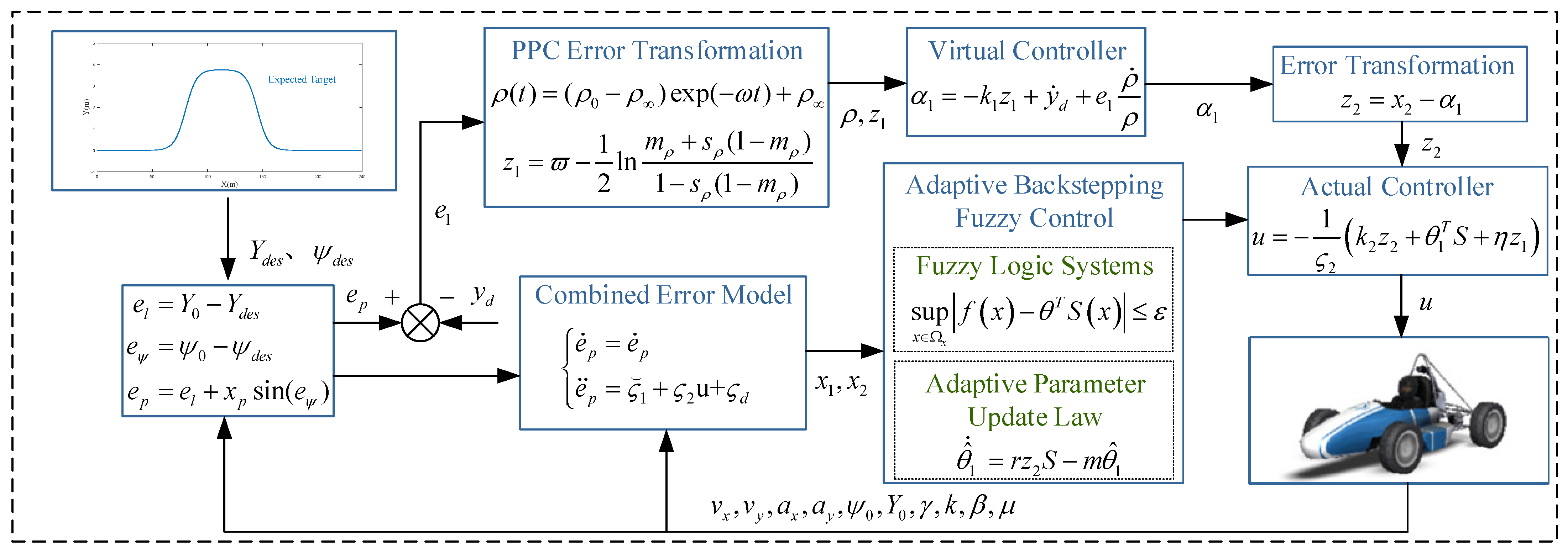
In this section, the prescribed performance adaptive backstepping fuzzy control method is introduced as a whole. The overall design architecture is shown in Figure 3. Based on the environmental perception system and the decision-making planning system, the expected lateral position and heading angle are planned. The difference between the actual lateral position and heading angle of the vehicle is taken to obtain the required combined error. The strict feedback model is applied to receive the current state information of the vehicle in real time and provide it to the controller. The combined error is processed with prescribed performance, and the virtual control law is derived using the backstepping method. Since it is difficult to obtain the derivative of the virtual control law and handle the disturbance and nonlinear terms in the controller, the adaptive update law and FLS are used to approximate them. Then, the real control law is derived using Lyapunov theory [31]. Finally, the real control law is connected to CarSim, and the real-time vehicle parameters and state information are fed back to the controller to form a closed loop of vehicle trajectory tracking control.

According to the combined error model (10), the true control model can be expressed as

$$\left\{\begin{array}{l}{\dot{x}}_1=x_2\\ {\dot{x}}_2={\stackrel{⌣}{\varsigma }}_1+{\varsigma }_2\mathrm{u}+{\varsigma }_d\\ y=x_1\end{array}\right.$$

(11)

A new coordinate transformation is proposed for the control system (11) as follows:

$$\left\{\begin{array}{l}{z}_1=\varpi -\left(\ln \left[m_{\rho }+s_{\rho }(1-m_{\rho })\right]/\left[1-s_{\rho }(1-m_{\rho })\right]\right)/2\\ z_2=x_2-{\alpha }_1\end{array}\right.$$

(12)

where ${\alpha }_1$ is the virtual control law that needs to be designed, and $\varpi$ is an important variable in the prescribed performance control, which will be explained in the next section.

3.1. Prescribed Performance Function and Error Transformation

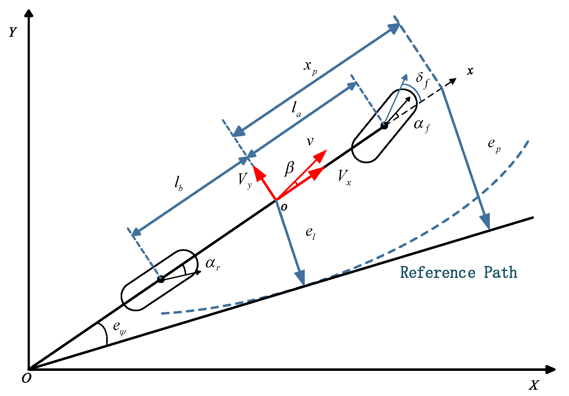
In the lateral control of vehicles, the values of the lateral position error $e_l$ and the heading angle error $e_{\psi }$ are of great significance to the accuracy and stability of vehicle trajectory tracking control. The tracking error is set to $e_i\left(t\right)=y_i-y_d$. The tracking error is required to meet the prescribed performance. If the following conditions are met, the requirements of the prescribed performance will be satisfied:

$$-\left[m_{\rho }+s_{\rho }(1-m_{\rho })\right]{\rho }_i(t)<e_i(t)<{\rho }_i(t)\left[1-s_{\rho }(1-m_{\rho })\right]$$

(13)

where the coefficient $m_{\rho }\in \left(0\right.,\left.1\right]$ is a positive number, $s_{\rho }$ adjusting the constraint performance according to the initial conditions of $e_i\left(t\right)$, $s_{\rho }$ can be expressed as

$$s_{\rho }=\left\{\begin{array}{l}0,e_i(0)\ge 0\\ 1,e_i(0)<0\end{array}\right.$$

(14)

This paper adopts a continuous prescribed performance function to constrain the combined error $e_p$ [32]. Where $e_p=e_l+x_p{e}_{\psi }$, according to the literature, the prescribed performance function is designed as follows

$${\rho }_i(t)=({\rho }_{0i}-{\rho }_{\infty i})\exp (-{\omega }_{i}t)+{\rho }_{\infty i},t\ge 0,i=1,2,\dots ,n$$

(15)

where coefficient ${\rho }_{0i},{\rho }_{\infty i}$ and ${\omega }_i$ are positive constants. ${\rho }_{0i},{\rho }_{\infty i}$ represent the values at $t=0$ and $t\to +\infty$, respectively. These coefficients satisfy ${\rho }_{0i}>{\rho }_{\infty i}$ and ${\rho }_{0i}>e_i\left(0\right)$.

The prescribed performance function quantifies the performance of $e_i\left(t\right)$, where the maximum overshoot of the tracking error does not exceed $m_{\rho }{\rho }_{0i}$, ${\rho }_{\infty i}$ is the upper bound of the steady-state error, and ${\omega }_i$ is the lower bound of the convergence rate.

Start the error transformation, transform the constrained error $e_1$ into an unconstrained error [33]

$$e_1(t)=\rho (t)\Theta (\varpi )$$

(16)

where $\Theta (\varpi )$ is defined as follows

$$\Theta (\varpi )={\displaystyle \frac{\left[1-s_{\rho }(1-m_{\rho })\right]\exp (\varpi )-\exp (-\varpi )\left[m_{\rho }+s_{\rho }(1-m_{\rho })\right]}{\exp (\varpi )+\exp (-\varpi )}}$$

(17)

When the values of $\varpi \to -\infty$ and $\varpi \to +\infty$ can, respectively, approximate the prescribed minimum and maximum error values, and it can be ensured that the unconstrained error signal $e_1$ can be within the prescribed error boundaries. When $\varpi =\left(ln\left[m_{\rho }+s_{\rho }\left(1-m_{\rho }\right)\right]/\left[1-s_{\rho }\left(1-m_{\rho }\right)\right]\right)/2$, the error can converge to zero.

Since the error transformation function $\Theta (\varpi )$ is strictly increasing, its inverse function can be expressed as

$$\varpi ={\Theta }^{-1}\left({\displaystyle \frac{e_1}{\rho }}\right)={\displaystyle \frac{1}{2}}\ln \left({\displaystyle \frac{\left[m_{\rho }+s_{\rho }(1-m_{\rho })\right]\rho +e_1}{\left[1-s_{\rho }(1-m_{\rho })\right]\rho -e_1}}\right)$$

(18)

The derivative of the transformation error $\varpi$ can be described as follows:

$$\dot{\varpi }={\displaystyle \frac{1}{\rho }}\left(\rho {\dot{e}}_1-e_1\dot{\rho }\right)\left({\displaystyle \frac{1}{2\left[\left(m_{\rho }+s_{\rho }(1-m_{\rho })\right)\rho +e_1\right]}}-{\displaystyle \frac{1}{2\left[e_1-\left(1-s_{\rho }(1-m_{\rho })\right)\rho \right]}}\right)$$

(19)

To simplify the (19), define $\dot{\varpi }=\eta \left(\rho {\dot{e}}_1-e_1\dot{\rho }\right)/\rho$, where

$$\eta =1/2\left[\left(m_{\rho }+s_{\rho }(1-m_{\rho })\right)\rho +e_1\right]-1/2\left[e_1-\left(1-s_{\rho }(1-m_{\rho })\right)\rho \right]>0$$

(20)

In conclusion, the specified performance function clearly defines the dynamic performance requirements for the combined error, and the quantified error provides an explanation for the coordinate transformation mentioned earlier, laying the foundation for the subsequent controller design.

3.2. Fuzzy Logic System

Fuzzy logic systems can approximate unknown functions to replace unknown functions or nonlinear functions. Therefore, the FLS will be applied in the control algorithm to be formulated subsequently. The FLS will be used to approximate the unknown nonlinear functions defined on certain compact sets. The following fuzzy rules will be derived by using the center average defuzzifier, product inference rule, and singleton fuzzification [34].

$$\begin{gathered} R_i: \mathrm{IF} x_1 \mathrm{is} F_1^i \mathrm{and} x_2 \mathrm{is} F_2^i \mathrm{and}\dots \mathrm{and}{x}_n \mathrm{is} F_n^i \\ \mathrm{Then} y \mathrm{is} B^i (i=1,2,\dots \mathrm{N}) \end{gathered}$$

(21)

where $x=\left[x_1,x_2,\dots ,x_n\in R^n\right]$ and $y\in R$ are the input and output of the fuzzy system, respectively. In this paper, the method of single-element fuzzification, product inference rules, and center average defuzzification is adopted. Thus, the output of the FLS can be expressed as

$$y\left(x\right)={\displaystyle \frac{{\displaystyle {\sum }_{j=1}^N{\overline{y}}^j{\displaystyle {\prod }_{i=1}^n{u}_{F_i^j}\left(x_i\right)}}}{{\displaystyle {\sum }_{j=1}^N\left({\displaystyle {\prod }_{i=1}^n{u}_{F_i^j}\left(x_i\right)}\right)}}}$$

(22)

In practical engineering applications, the controller combined with the FLS needs to be repeatedly adjusted based on actual conditions and experience, as many parameters in the control system require improvement and debugging, and some values need to be constantly corrected. To meet such requirements, this paper adopts an adaptive fuzzy logic system, and (22) can be rewritten as

$$y\left(x\right)={\theta }^{T}S(x)$$

(23)

where $\theta ={\left[{\overline{y}}^1,{\overline{y}}^2,\dots ,{\overline{y}}^N\right]}^T$ is an adjustable parameter in the adaptive system, and $S\left(x\right)={\left[S^1\left(x\right),S^2\left(x\right),\dots ,S^N\left(x\right)\right]}^T$ is the fuzzy basis function vector, where the fuzzy basis function is defined as

$$S^j\left(x\right)={\displaystyle \frac{{\displaystyle {\prod }_{i=1}^n{u}_{F_i^j}\left(x_i\right)}}{{\displaystyle {\sum }_{j=1}^N\left({\displaystyle {\prod }_{i=1}^n{u}_{F_i^j}\left(x_i\right)}\right)}}}$$

(24)

If all the membership functions are chosen as Gaussian functions, the following lemma holds.

Lemma 1. 

In [35], the authors state that for an arbitrarily small approximation error, i.e., $\forall {\epsilon }_0>0$, there always exists an FLS that can uniformly approximate any real continuous function $f\left(x\right):R^n\to R$ in a compact set ${\Omega }_x\in R^n$, i.e.,

$$\underset{x\in {\Omega }_x}{\sup }\left|f\left(x\right)-{\theta }^{T}S\left(x\right)\right|\le \epsilon$$

(25)

where $\epsilon$ is the minimum estimation error, the expression form of the FLS can be rewritten as

$$f\left(x\right)={\theta }^{T}S\left(x\right)+\epsilon$$

(26)

there exists an upper bound for $\epsilon$, which can be expressed as $\epsilon \le \overline{\epsilon }$.

Lemma 2. 

In [36], the authors state that Young’s inequality can be described as follows:

$${\left|\vartheta \right|}^{\xi }{\left|\Gamma \right|}^o\le {\displaystyle \frac{\xi }{\xi +o}}\chi {\left|\vartheta \right|}^{\xi +o}+{\displaystyle \frac{o}{\xi +o}}{\chi }^{{\displaystyle \frac{-\xi }{o}}}{\left|\Gamma \right|}^{o+\xi }$$

(27)

where $\xi ,o,\chi$ are any given positive constants, and $\vartheta ,\Gamma$ are real variables.

FLS mainly deals with the nonlinear terms and disturbance terms in the subsequent controller. Lemmas 1 and 2 will play a crucial role in the stability analysis.

3.3. PPC-ABFC Controller Design

The above are the theorems and theories required for the controller. Below, a prescribed performance adaptive backstepping fuzzy controller will be designed. The main steps are as follows:

STEP 1. Select the Lyapunov function

$$V_1={\displaystyle \frac{1}{2}}{z}_1^2$$

(28)

Differentiate (28) yields

$${\dot{V}}_1=z_1{\dot{z}}_1=z_1\eta \left(z_2+{\alpha }_1-{\dot{y}}_d-e_1{\displaystyle \frac{\dot{\rho }}{\rho }}\right)$$

(29)

The virtual control law is designed as

$${\alpha }_1=-k_1{z}_1+{\dot{y}}_d+e_1{\displaystyle \frac{\dot{\rho }}{\rho }}$$

(30)

where $\dot{\rho }=-\varpi \left({\rho }_0-{\rho }_{\infty }\right)\exp \left(-\varpi t\right)$, and $k_1$ is the positive constant of the design.

Substituting (30) into (29) yields

$$\begin{array}{cc}\hfill {\dot{V}}_1& =z_1\eta \left(z_2+{\dot{y}}_d-k_1{z}_1+e_1{\displaystyle \frac{\dot{\rho }}{\rho }}-{\dot{y}}_d-e_1{\displaystyle \frac{\dot{\rho }}{\rho }}\right)\hfill \\ \hfill & =-\eta k_1{z}_1^2+\eta z_1{z}_2\hfill \end{array}$$

(31)

STEP 2. According to the adaptive parameter update law, take the Lyapunov function

$$V_2={\displaystyle \frac{1}{2}}{z}_2^2+{\displaystyle \frac{1}{2r}}{\tilde{\theta }}_1^T{\tilde{\theta }}_1$$

(32)

where $r>0$ can be designed, ${\tilde{\theta }}_1={\theta }_1-{\widehat{\theta }}_1$, ${\widehat{\theta }}_1$ is the estimated value of ${\theta }_1$, ${\tilde{\theta }}_1$ is the estimated error value. According to (11) and (12), the following can be obtained:

$${\dot{z}}_2={\stackrel{⌣}{\varsigma }}_1+{\varsigma }_{2}u+{\varsigma }_d-{\dot{\alpha }}_1$$

(33)

The time differentiation of (32) yields

$$\begin{array}{cc}\hfill {\dot{V}}_2& =z_2{\dot{z}}_2-{\displaystyle \frac{1}{r}}{\tilde{\theta }}_1^T{\dot{\widehat{\theta }}}_1\hfill \\ \hfill & =z_2\left({\stackrel{⌣}{\varsigma }}_1+{\varsigma }_{2}u+{\varsigma }_d-{\dot{\alpha }}_1\right)-{\displaystyle \frac{1}{r}}{\tilde{\theta }}_1^T{\dot{\widehat{\theta }}}_1\hfill \end{array}$$

(34)

Since it is difficult to determine the derivative of ${\alpha }_1$ and also to handle the uncertain parameters and disturbance terms in the model, the definition is given as follows:

$$f_1={\stackrel{⌣}{\varsigma }}_1+{\varsigma }_d-{\dot{\alpha }}_1$$

(35)

According to Lemma 1, for any given ${\epsilon }_1$, there is an FLS ${\theta }^{T}S\left(x\right)$, for distance, $f_1={\theta }_1^{T}S\left(x\right)+{\epsilon }_1$, ${\epsilon }_1$ represents the error of approximation and satisfies $\Vert {\epsilon }_1\Vert <{\overline{\epsilon }}_1({\overline{\epsilon }}_1>0)$.

Substituting (35) into (34) yields

$${\dot{V}}_2=z_2\left({\varsigma }_{2}u+{\theta }_1^{T}S+{\epsilon }_1\right)-{\displaystyle \frac{1}{r}}{\tilde{\theta }}_1^T{\dot{\widehat{\theta }}}_1$$

(36)

The real control law and adaptive parameter update law of the trajectory tracking control system are proposed as follows:

$$\left\{\begin{array}{l}u=-{\displaystyle \frac{1}{{\varsigma }_2}}\left(k_2{z}_2+{\theta }_1^{T}S+\eta z_1\right)\\ {\dot{\widehat{\theta }}}_1=r{z}_{2}S-m{\widehat{\theta }}_1\end{array}\right.$$

(37)

where $k_2$ is a positive parameter that can be designed, $r$ is the learning law in the adaptive parameter update law, and $m>0$.

Substituting (37) into (36) yields

$$\begin{array}{cc}\hfill {\dot{V}}_2& =z_2({\varsigma }_2(-{\displaystyle \frac{1}{{\varsigma }_2}}(k_2{z}_2+{\theta }_1^{T}S+\eta z_1))+{\theta }_1^{T}S\hfill \\ \hfill & +{\epsilon }_1)-{\displaystyle \frac{1}{r}}{\tilde{\theta }}_1^T\left(r{z}_{2}S-m{\widehat{\theta }}_1\right)\hfill \\ \hfill & =z_2((-k_2{z}_2-{\theta }_1^{T}S-\eta z_1)+{\theta }_1^{T}S+{\epsilon }_1)\hfill \\ \hfill & -z_2{\tilde{\theta }}_1^{T}S+{\displaystyle \frac{1}{r}}m{\tilde{\theta }}_1^T{\widehat{\theta }}_1\hfill \\ \hfill & ={\displaystyle \frac{1}{r}}m{\tilde{\theta }}_1^T{\widehat{\theta }}_1-k_2{z}_2^2-\eta z_1{z}_2+z_2{\epsilon }_1\hfill \end{array}$$

(38)

STEP 3. Stability analysis

Theorem 1. 

For the trajectory tracking control system, considering the virtual control law (30), the actual control law, the adaptive parameter update law (37), and the error transformation (12), it can be guaranteed that the error converges to a small neighborhood around the origin, and all signals within the closed-loop system are Lyapunov stable.

Proof of Theorem 1. 

Design a Lyapunov function $V=V_1+V_2$. Taking the derivative of $V$, substituting (31) into (38) yields

$$\begin{array}{cc}\dot{V}& ={\dot{V}}_1+{\dot{V}}_2\hfill \\ \hfill & =-\eta k_1{z}_1^2+\eta z_1{z}_2+{\displaystyle \frac{1}{r}}m{\tilde{\theta }}_1^T{\widehat{\theta }}_1-k_2{z}_2^2-\eta z_1{z}_2+z_2{\epsilon }_1\hfill \\ \hfill & =z_2{\epsilon }_1-\eta k_1{z}_1^2-k_2{z}_2^2+{\displaystyle \frac{1}{r}}m{\tilde{\theta }}_1^T{\widehat{\theta }}_1\hfill \end{array}$$

(39)

According to Young’s inequality, the following can be obtained:

$$\left\{\begin{array}{l}{\displaystyle \frac{m}{r}}{\tilde{\theta }}_1^T{\widehat{\theta }}_1={\displaystyle \frac{m}{r}}{\tilde{\theta }}_1^T\theta -{\displaystyle \frac{m}{r}}{\tilde{\theta }}_1^T\tilde{\theta }\le {\displaystyle \frac{m}{2r}}{\tilde{\theta }}_1^T{\tilde{\theta }}_1+{\displaystyle \frac{m}{2r}}{\theta }_1^T{\theta }_1-{\displaystyle \frac{m}{r}}{\tilde{\theta }}_1^T{\tilde{\theta }}_1\\ \hspace{1em} =-{\displaystyle \frac{m}{2r}}{\tilde{\theta }}_1^T{\tilde{\theta }}_1+{\displaystyle \frac{m}{2r}}{\theta }_1^T{\theta }_1\\ z_2{\epsilon }_1\le {\displaystyle \frac{1}{2}}{z}_2^2+{\displaystyle \frac{1}{2}}{\epsilon }_1^2\le {\displaystyle \frac{1}{2}}{z}_2^2+{\displaystyle \frac{1}{2}}{\overline{\epsilon }}_1^2\end{array}\right.$$

(40)

Substituting (40) into (39) yields

$$\begin{array}{cc}\dot{V}& \le {\displaystyle \frac{1}{2}}{z}_2^2+{\displaystyle \frac{1}{2}}{\overline{\epsilon }}_1^2-\eta k_1{z}_1^2-k_2{z}_2^2-{\displaystyle \frac{m}{2r}}{\tilde{\theta }}_1^T{\tilde{\theta }}_1+{\displaystyle \frac{m}{2r}}{\theta }_1^T{\theta }_1\hfill \\ \hfill & \le -\eta k_1{z}_1^2-(k_2-{\displaystyle \frac{1}{2}})z_2^2-{\displaystyle \frac{m}{2r}}{\tilde{\theta }}_1^T{\tilde{\theta }}_1+{\displaystyle \frac{m}{2r}}{\theta }_1^T{\theta }_1+{\displaystyle \frac{1}{2}}{\overline{\epsilon }}_1^2\hfill \\ \hfill & \le -\kappa V+M_0\hfill \end{array}$$

(41)

where

$$\begin{array}{l}\kappa =\min [2\eta k_1,2(k_2-{\displaystyle \frac{1}{2}}),m]\\ M_0={\displaystyle \frac{m}{2r}}{\theta }_1^T{\theta }_1+{\displaystyle \frac{1}{2}}{\overline{\epsilon }}_1^2\end{array}$$

(42)

By integrating (42), it follows that

$$\begin{array}{cc}\hfill V(t)& \le V(0)\exp (-\kappa t)+{\displaystyle \frac{M_0}{\kappa }}(1-\exp (-\kappa t))\hfill \\ \hfill & \le V(0)+{\displaystyle \frac{M_0}{\eta }}\hfill \end{array}$$

(43)

Through the above equation, it can be obtained that when $t\to \infty , V\to M_0/\kappa$. Furthermore, $z_1,z_2,\tilde{\theta },{\alpha }_1,u$ are bounded, and all estimated values of the parameters are also bounded. From the fact that $z_1$ and coordinate transformation, it can also be concluded that $x_1$ is bounded. From the fact that $z_1,z_2$ and coordinate transformation, it can also be concluded that $x_2$ is bounded. From the fact that $z_1,z_2,\tilde{\theta }$ is bounded, it can also be concluded that $u$ is bounded. Moreover, all signals in this system are bounded.

According to (43) and the derivative of $V$, the following can be obtained:

$$z_1^2\le 2\left[V(0)\exp (-\kappa t)+M_0(1-\exp (-\kappa t))/\kappa \right]$$

(44)

It can be seen from (44) that $z_1$ converges to a compact set.

$$Z_e=\left\{z_1:‖z_1‖\le {(2M_0/\kappa )}^{1/2}\right\}$$

(45)

Furthermore, the transformed variable $\varpi$ is also bounded. Theorem 1 is proved. □

Remark 1. 

This compact set $Z_e$ is associated with unknown bounded term $M_0$ and negative definite term $\kappa$. $\kappa$ is associated with $\eta ,m,k_1$ and $k_2$. All these parameters are adjustable. Even if the specific value of $M_0$, the parameters related to $M_0$ and $\kappa$ can be adjusted. This can make the compact set $Z_e$ as small as possible.

4. Simulation Results

In this section, in order to illustrate the effectiveness of vehicle trajectory tracking, the lateral controller (prescribed performance adaptive backstepping fuzzy control, PPC-ABFC) is verified through co-simulation using CarSim–Simulink. A high-fidelity racing car model is established in CarSim, with the power source of the CarSim model being the same as that of the racing car, both being rear-mounted motor-driven. Simulink receives the state signals from CarSim, and then Simulink generates control signals to input into CarSim, forming a control loop. The road adhesion coefficient is 0.85, and two different vehicle speeds are set to verify the robustness of the controller.

The membership function of the fuzzy logic system is selected as the Gaussian function. This is because the Gaussian function can produce smooth and continuous membership output and is computationally efficient, which is crucial for vehicle dynamics control. Based on a large body of literature (such as [37,38]) and engineering practices, it has been demonstrated to have excellent performance in handling problems such as trajectory tracking and nonlinear systems. The Gaussian function is as follows:

$$u_{F_i^j}=\exp \left(-{\displaystyle \frac{1}{2}}{(x_i-c_j)}^2\right)$$

(46)

where $c_j={\left[c_1,c_2,\dots ,c_{13}\right]}^T$ is the center.

To verify the PPC-ABFC controller, the commonly used double-lane-change maneuver was selected for verification. The expected lateral position and the expected heading angle are given by the following formulas.

$$\left\{\begin{array}{l}{Y}_{des}={\displaystyle \frac{1}{2}}{r}_{y1}[1+\tanh (d_{y1})]-{\displaystyle \frac{1}{2}}{r}_{y2}[1+\tanh (d_{y2})]\\ {\psi }_{des}=\arctan [r_{y1}{({\displaystyle \frac{1}{\cosh (d_{y1})}})}^2({\displaystyle \frac{1.2}{r_{x1}}})-r_{y2}{({\displaystyle \frac{1}{\cosh (d_{y1})}})}^2({\displaystyle \frac{1.2}{r_{x2}}})]\end{array}\right.$$

(47)

where $r_{y1}=r_{y2}=3.76,r_{x1}=r_{x2}=25,d_{y1}=0.1\left(x-68\right)-1.2,d_{y2}=0.1\left(x-133\right)-1.2$.

This article will introduce four performance indicators to evaluate the performance of the three controllers, including the root-mean-square error (RMSE): $\mathrm{RMSE}={\left({\displaystyle \frac{1}{n}}{{\displaystyle \sum }}_{i=1}^n{e}_i^2\right)}^{0.5}$; the maximum absolute error (MAE): $\mathrm{MAE}=ma{x}_{i=1\cdots n}\left\{\left|e_i\right|\right\}$; the standard deviation (SD): $\mathrm{SD}={\left({{\displaystyle \sum }}_{i=1}^n{\left(e_1-\overline{e}\right)}^2/n\right)}^{0.5}$; and the variance (VAR): $\mathrm{VAR}=\left({{\displaystyle \sum }}_{i=1}^n{\left(e_i-\overline{e}\right)}^2\right)/n$.

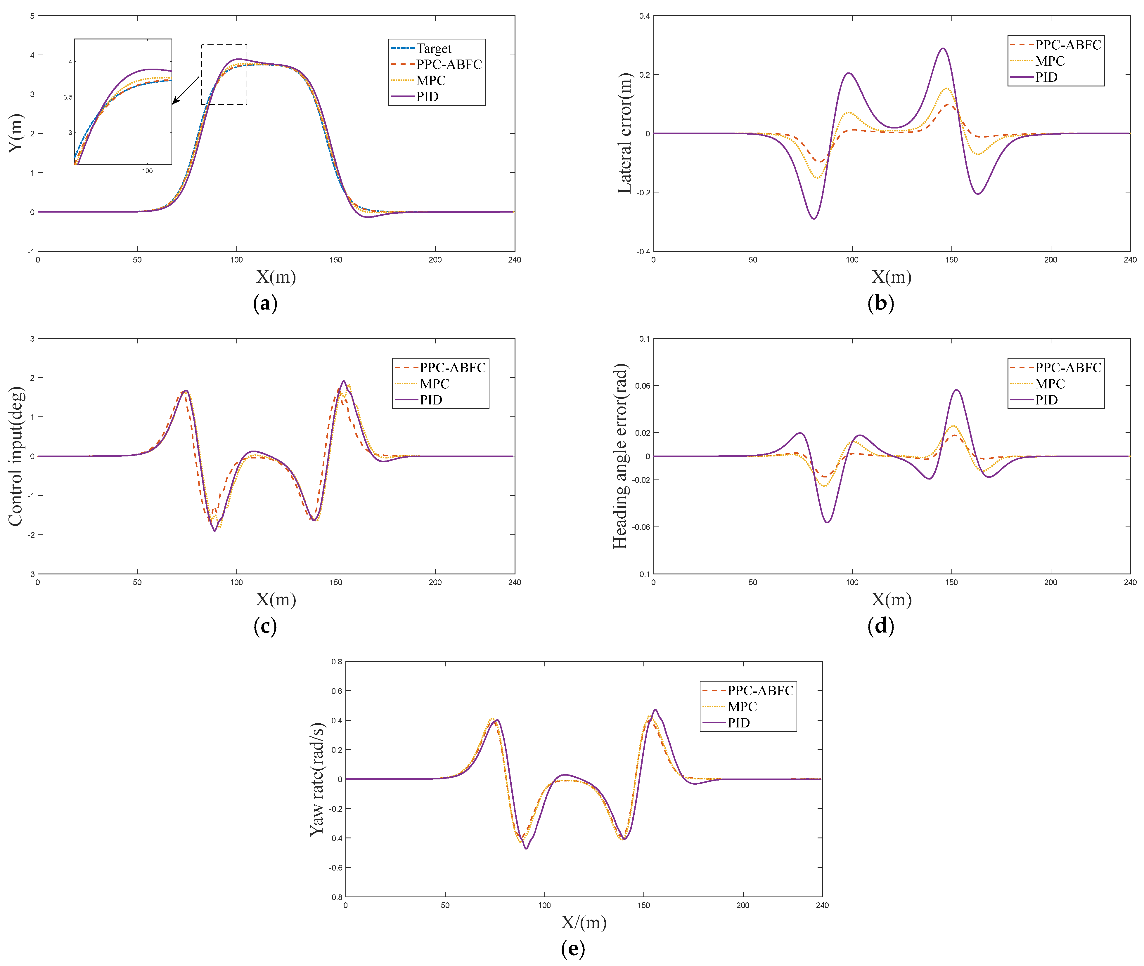
Conduct trajectory tracking simulation experiments and make comparisons, respectively, at speeds of 60 km/h and 100 km/h. Figure 4 shows the simulation experiment at a vehicle speed of 60 km/h. Moreover, this paper sets up two comparative experiments to verify the superiority of PPC-ABFC. The parameters of PPC-ABFC are selected as: $x_p=8, m=110, r=20, k_1=10, k_2=50,m_{\rho }=1$. Since the prescribed performance function requires setting the initial error and the error when $t\to \infty$, if the numerical values are set too small, it will cause the controller to oscillate. Therefore, the parameters are selected as ${\rho }_0=10,{\rho }_{\infty }=3,\omega =1$. The first set of comparative experiments aimed to verify the role of PPC technology in the scheme proposed in this paper. An adaptive backstepping fuzzy controller (ABFC) without PPC was redefined. The second set of comparative experiments (the abbreviation for the controller is BFC) aimed to verify the significance of the FLS’s approximation of unknown nonlinear terms. The prescribed performance is removed, and the adaptive FLS also does not approximate the unknown nonlinear terms and disturbance terms, but only the derivative of ${\alpha }_1$. To ensure fairness among different controllers, the other parameters are designed in a consistent manner. All the experimental conditions, trajectory tracking paths, vehicle models, and operating environments remained consistent.

Figure 4 shows the control effects of the three controllers during trajectory tracking. Figure 4a shows an expected trajectory and the tracking effects of three controllers. It can be seen from the figure that the designed PPC-ABFC controller has a better tracking effect than the other two control algorithms when tracking the expected trajectory. Figure 4b shows the comparison of the lateral error of the vehicle during trajectory tracking. Lateral error is the most effective indicator of the vehicle’s trajectory tracking performance.

It can be visually observed from the graph that the control error of the PPC-ABFC is smaller than that of the other two comparison controllers. Moreover, a data comparison of the lateral error of the vehicle was conducted, as shown in

Table 2. Comparison of lateral error performance indicators of three controllers in the simulation experiment at a vehicle speed of 60 km/h.

Methods	PPC-ABFC	ABFC	BFC
RMSE	0.0121	0.0287	0.0575
MAE	0.0423	0.0772	0.1712
SD	0.0121	0.0287	0.0575
VAR	1.465 × 10−4	8.220 × 10−4	0.0033

. The RMSE, MAE, SD, and VAR of the four performance indicators of PPC-ABFC were all smaller than those of ABFC and BFC. Figure 4c shows the input values of CarSim. It is obvious that the input values of PPC-ABFC are more stable than the other two. The adjustment of PPC-ABFC is also more stable at 100–120 m. Figure 4d shows the comparison of heading angle errors. It can be seen intuitively that the control effect of the designed PPC-ABFC controller on the heading angle is better than the other two controllers. Combining Figure 4b and Figure 4d, it can be concluded that the combined error during PPC-ABFC control is also smaller than that of the other two controllers.

Figure 4e shows the comparison of the yaw rate of the vehicle. It can be seen from the figure that the value of PPC-ABFC is slightly higher than that of the other two controllers. This is because the trajectory of the vehicle under this controller is very close to the expected trajectory, so it is slightly higher, which does not mean that the control effect is poor. On the contrary, the control effect of PPC-ABFC is more stable than the other two. From this, it can be seen that FLS can effectively approximate the nonlinear and disturbance terms in the vehicle model, successfully compensating for the model’s uncertainty and making the output of the controller more stable while also increasing the control accuracy. In conclusion, the control performance of PPC-ABFC meets the design requirements.

Remark 2. 

$k_1$ and $k_2$ are the main adjustment parameters of the controller. When other parameters remain constant, appropriately increasing $k_1$ can reduce the error, and increasing $k_2$ can enhance the stability of the controller’s output value. However, the adjustment should not be too large. When $k_1$ is greater than around 50 or $k_2$ is greater than around 200, the entire control system will experience jitter. ${\rho }_0, {\rho }_{\infty },\omega$—these are all important parameters of PPC. ${\rho }_0$ represents the initial error, and it needs to be as large as possible to ensure that the initial error remains within the preset range. The value of ${\rho }_{\infty }$ should be less than that of ${\rho }_0$, but it cannot be too small, because an excessively small value would cause jittering, which could lead to the error exceeding the performance limit suddenly. $\omega$ is used to ensure the convergence speed. The value of $\omega$ can be appropriately increased, which will enhance the convergence speed. However, it cannot be set too large, as this would cause the convergence rate to be too fast, resulting in instability in the controller. The parameters $r$ and $m$ in the adaptive rules are crucial. Increasing $r$ can accelerate the convergence of weights, but if it is too large, it will lead to overshoot and oscillation. Increasing $m$ can enhance the stability of the system, but if it is too large, instability will occur.

The following is a simulation test under high-speed conditions, with a vehicle speed of 100 km/h. The PID control algorithm and the MPC algorithm were set up for comparison with PPC-ABFC. Moreover, in this group of experiments, a time calculation cost performance index was added to verify that the PPC-ABFC algorithm is superior to the MPC algorithm in terms of time cost. In Figure 5a, the blue line represents the expected trajectory, the purple line shows the trajectory tracking effect of the vehicle under the PID controller, the orange line indicates the trajectory tracking effect under the PPC-ABFC controller, and the yellow line indicates the trajectory tracking effect under the MPC controller. It can be clearly observed that when the vehicle is running at high speed, the PID controller causes vehicle instability near 100 m and 160 m of the curve, while the PPC-ABFC controller does not experience instability and instead achieves a relatively good tracking effect. Although the MPC controller did not exhibit instability, its control accuracy was slightly lower than that of the PPC-ABFC.

Figure 5b shows the comparison of lateral errors of the vehicle during trajectory tracking.

Table 3. Comparison of lateral error performance indicators and total time cost of the three controllers in the simulation experiment at a vehicle speed of 100 km/h.

Methods	PPC-ABFC	MPC	PID
RMSE	0.0286	0.0473	0.1072
MAE	0.0981	0.1526	0.2900
SD	0.0286	0.0473	0.1072
VAR	8.168 × 10−4	0.0022	0.0115
Total Time Cost (s)	2.763	1.690	1 × 10−3

illustrates that the maximum lateral error under the PPC-ABFC strategy is only 0.0981 m, which is much smaller than the control error under the PID controller and also less than the lateral error value of 0.1526 under the MPC strategy. Moreover, a data comparison was conducted, and the RMSE, MAE, SD, and VAR of the four performance indicators of PPC-ABFC were all smaller than those of PID and MPC. Figure 5c is a comparison chart of the control input. The input values of CarSim are shown in the figure. It can be observed that although there is some jitter when using PPC-ABFC control, the overall control input is relatively stable. In contrast, under PID control, the control input shows a reverse value at 170 m.

Moreover, the MPC also experienced shaking when turning. Figure 5d is a comparison chart of heading angle error. It can be observed that the control error of the designed PPC-ABFC controller is smaller than that of the PID and MPC controllers. Combining Figure 5b and Figure 5d, the combined error under PPC-ABFC control is smaller than that of the PID and MPC controllers.

Figure 5e is a comparison chart of yaw rate. It can be observed that when PPC-ABFC control is applied, the yaw rate is lower than that under PID control, indicating that the vehicle’s stability is superior to that under PID control. The yaw rate under the MPC control strategy is also slightly greater than that under PPC-ABFC. Thus, it can be seen that the vehicle’s driving is more stable under the PPC-ABFC control. In Table 3, the total running time cost of each controller is shown. It can be seen that the time cost of PPC-ABFC is 38.8% lower than that of MPC, and its control accuracy is also better than that of MPC. Although the PID algorithm requires very little time cost, it fails to achieve sufficient control accuracy in high-speed simulation scenarios, which may lead to vehicle safety hazards. In conclusion, the designed PPC-ABFC controller outperforms other control algorithms in tracking the expected trajectory during high-speed vehicle operation, and all the values are relatively good; the time cost is also lower than that of the comparison algorithm. It can be seen that the designed controller meets the expected effect.

5. Conclusions

In order to improve the control accuracy and ensure the stability of the vehicle during trajectory tracking of driverless electric formula racing cars, an adaptive backstepping fuzzy controller based on prescribed performance is proposed in this paper. This solves the problems of low control accuracy and instability of the vehicle while driving due to the generation of nonlinear terms, perturbations, and unknown parameters of the model when controlling the lateral movement of the driverless electric formula racing car. The FLS is utilized to approximate them, and the adaptive parameter update law is combined to adjust the parameters in real time. Combined with the prescribed performance function, the virtual control law and the real control law were designed through the backstepping method. The global asymptotic stability of the PPC-ABFC closed-loop system was proved by applying the Lyapunov stability theory. The vehicle model is built in CarSim, and the CarSim–Simulink co-simulation is conducted. The results show that PPC-ABFC can still exhibit good control performance at medium-high and high speeds. Compared with other controllers, it can be seen that the control accuracy and robustness of PPC-ABFC are both superior to the comparison control algorithms. The time cost is also lower than that of the MPC algorithm. This research provides a valuable reference for researchers in the field of unmanned vehicle trajectory tracking control to explore the application of intelligent nonlinear algorithms in this area. In the future, we will consider issues such as actuator failures, introduce fault-tolerant control, and explore fixed-time or finite-time stability theories to further optimize performance. We will also actively prepare a real vehicle to experiment with the proposed algorithm on real vehicles.