1. Introduction
Path planning in off-road environments refers to finding safe and efficient paths for vehicles in areas lacking established roads, crucial for emergency response in disaster events [
1,
2]. Off-road environments, typically located in remote or rural areas, often present a variety of complex and natural features and obstacles posing challenges to successful vehicles passing through [
3]. These challenges arise from two primary factors, including the complex nature of terrain features and the variability in the maneuverability of different vehicles under the complex and different land cover in off-road conditions (such as farmland, forest, grassland, shrubland, wetland etc.), complicating the developing generalizable and quantitative models for mobility analysis [
4]. Thus, quantifying the impacts of geographical factors on off-road mobility, developing universal models to map passable areas, and establishing path-planning algorithms specifically designed for off-road environments become important for efficient path planning [
5,
6].
Terrain modeling for off-road mobility focuses on understanding how terrain factors impact vehicle performance. These algorithms consider factors complicating mobility analysis for vehicles, including varying elevations, slopes, vegetation, vehicle capability, and potential obstacles to generate optimal paths [
7,
8]. Using binary classification (passable zones suitable for vehicle movement and obstacle zones) based on different land types to represent the environment is a common approach in off-road navigation tasks [
9,
10,
11,
12,
13]. Studies have emphasized the role of terrain attributes, such as Digital Elevation Models (DEMs) and soil types, in shaping off-road vehicle dynamics, while others systematically categorized these factors into six domains, including landforms, vegetation, land water systems, residential facilities, land transportation networks, and soil types [
14]. These foundational studies underscore the demand for a universal standard to quantify cross-region mobility, addressing complex interactions among terrain features and vehicle capabilities.
How to accurately represent the natural environment in a navigation system presents unique challenges for path planning in off-road environments. Traditional road navigation systems rely on topological graphs composed of edges (road segments) and nodes (intersections) to represent road networks [
15]. This approach cannot be directly applied to off-road settings due to the absence of a predefined road network. Although visibility graphs can be established by creating connectivity between significant landmarks, obstacles, or waypoints, the simplicity of topological graphs can lead to losses of details of the environment, potentially limiting the ability to find optimal paths or avoid obstacles that are not explicitly depicted in the graph [
16,
17]. Research has explored grid-based mesh and Voronoi diagrams to model off-road environments for path planning [
18,
19]. Grid-based models represent the environment as a grid of nodes and edges, where each grid cell corresponds to a node, and adjacent cells are connected by edges. Chen (2023) proposed a hexagonal grid-based approach for off-road path planning, highlighting its suitability for irregular terrains [
20]. Wu et al. (2024) introduced a hierarchical environmental modeling strategy, combining elevation and land cover data to generate multi-layer grid-based models, improving mobility analysis for off-road areas [
21]. Voronoi diagrams effectively partition free space into cohesive regions, where each region associates with a specific point or object, such as individual obstacles [
22]. The diagram edges highlight the collision-free paths. However, the diagram structure may not always align well with the terrain field, leading to unnecessary complexity [
23].
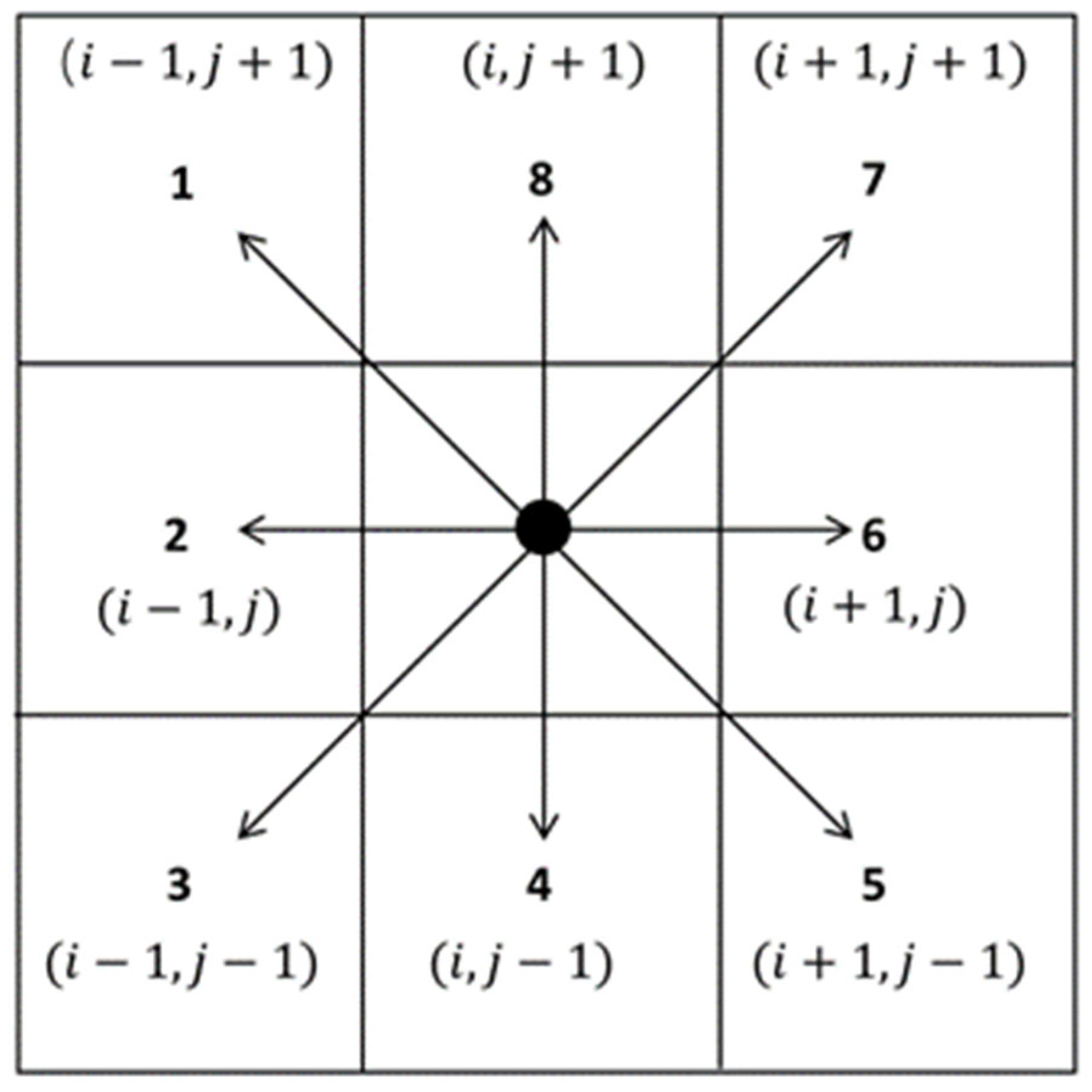
While 8-direction square grids have traditionally shown promise for off-road path planning [
24], recent studies have highlighted the potential of Delaunay triangulation NavMeshes for large-scale environment representation [
25]. Although studies have emphasized the effectiveness of grid-based systems on efficient grid connectivity and dynamic terrain adaptability for autonomous vehicles in rugged terrains [
26], the method is sensitive to the efficiency of path planning and can struggle to represent irregular obstacles accurately. Grid cells intersecting with obstacles are often marked as impassable, potentially limiting the feasible path space [
27]. A finer grid resolution offers a more detailed representation of the environment but demands greater computational resources, while a coarser resolution reduces storage and computational load but may fail to capture smaller obstacles [
28,
29]. Delaunay triangular NavMeshes, a well-established data structure in virtual environments, gaming, and indoor environments [
30,
31], offer a promising alternative for off-road path planning. By partitioning passable regions into convex polygons, Delaunay triangulation provides a more flexible and adaptive representation of terrain obstacles [
31,
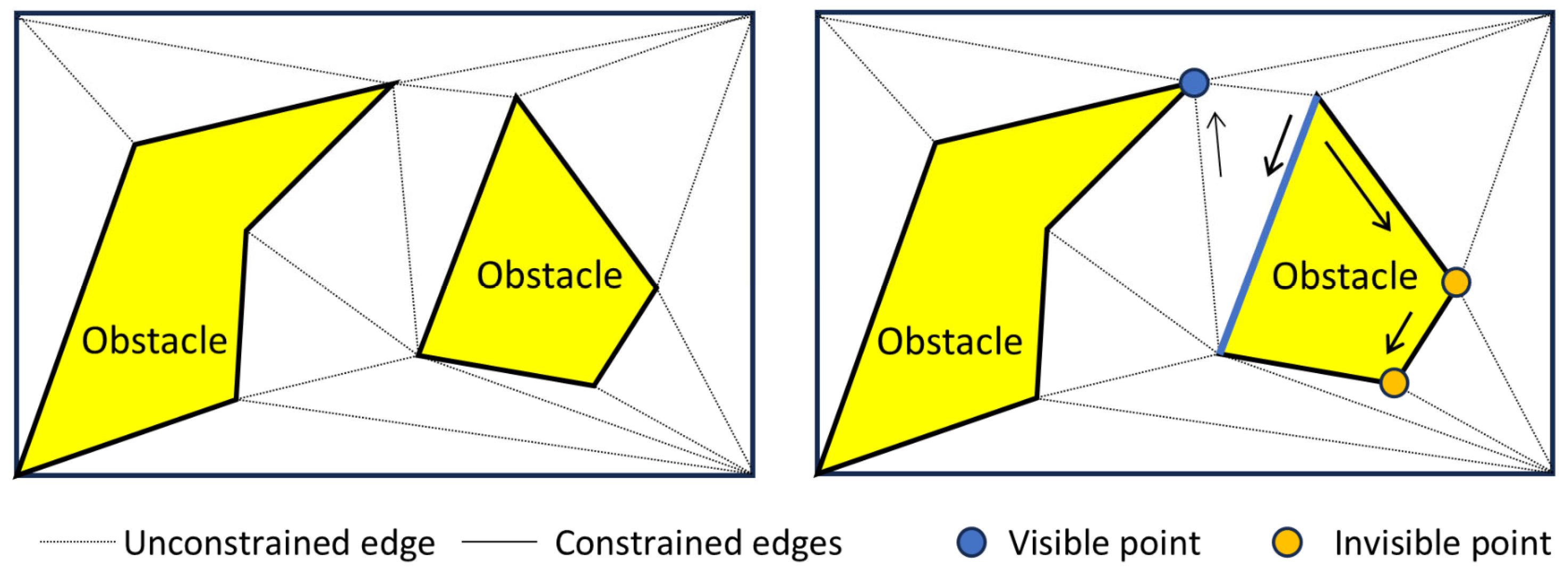
32]. Constrained Delaunay triangular NavMeshes ensure accurate alignment with obstacle boundaries, improving the representation of complex terrains. The unique properties of Delaunay triangulation, such as empty circle and max-min angle, contribute to efficient NavMeshes generation and smaller data representations [
33,
34]. However, the application of Delaunay triangulation to off-road scenarios remains relatively unexplored.
Various algorithms have been developed for off-road path planning in natural environments, each with distinct advantages and challenges. The A* algorithm is a well-known search method that efficiently finds optimal paths in grid-based environments. However, its performance degrades in dynamic or highly complex terrains, and its reliance on grid representations limits scalability [
35]. Variants like D* Lite improve on A* by enabling incremental updates for dynamic replanning, reducing computational costs in changing environments [
36]. Researchers have also explored advanced algorithms like Theta* and particle swarm optimization to improve computational efficiency in off-road environments. Theta* enhances path quality by allowing smoother, more direct routes through continuous space [
37]. Rapidly-Exploring Random Trees (RRT) excel in high-dimensional spaces but often produce suboptimal, winding paths [
38], while Artificial Potential Field (APF) methods can lead to path oscillations, increasing computation time and path length [
39]. Probabilistic Roadmaps (PRM) are useful for large spaces but suffer from inefficiency in complex environments [
40]. The Funnel Optimization algorithm addresses these challenges by combining global search with local optimization, balancing exploration and exploitation to produce smoother, more efficient paths in constrained environments [
41]. However, the application of Funnel Optimization to off-road scenarios remains relatively unexplored. Recently, several machine learning-assisted optimization methods have been introduced to enhance path planning performance in complex or unstructured environments. These include neural-network-based heuristics to accelerate search [
42], learning-based trajectory prediction to mimic human driving behavior [
43], and deep reinforcement learning for terrain-aware decision-making [
44]. It can be seen from the above literature [
42,
43,
44] that machine learning-based methods have great potential in off-road path planning. However, in emergency situations such as rescue operations, the shortest path needs to be found quickly. Path planning algorithms based on machine learning require high computational costs, which contradicts our scenario requirements. Additionally, due to the “black box effort” inherent in machine learning, it lacks the interpretability of the process.
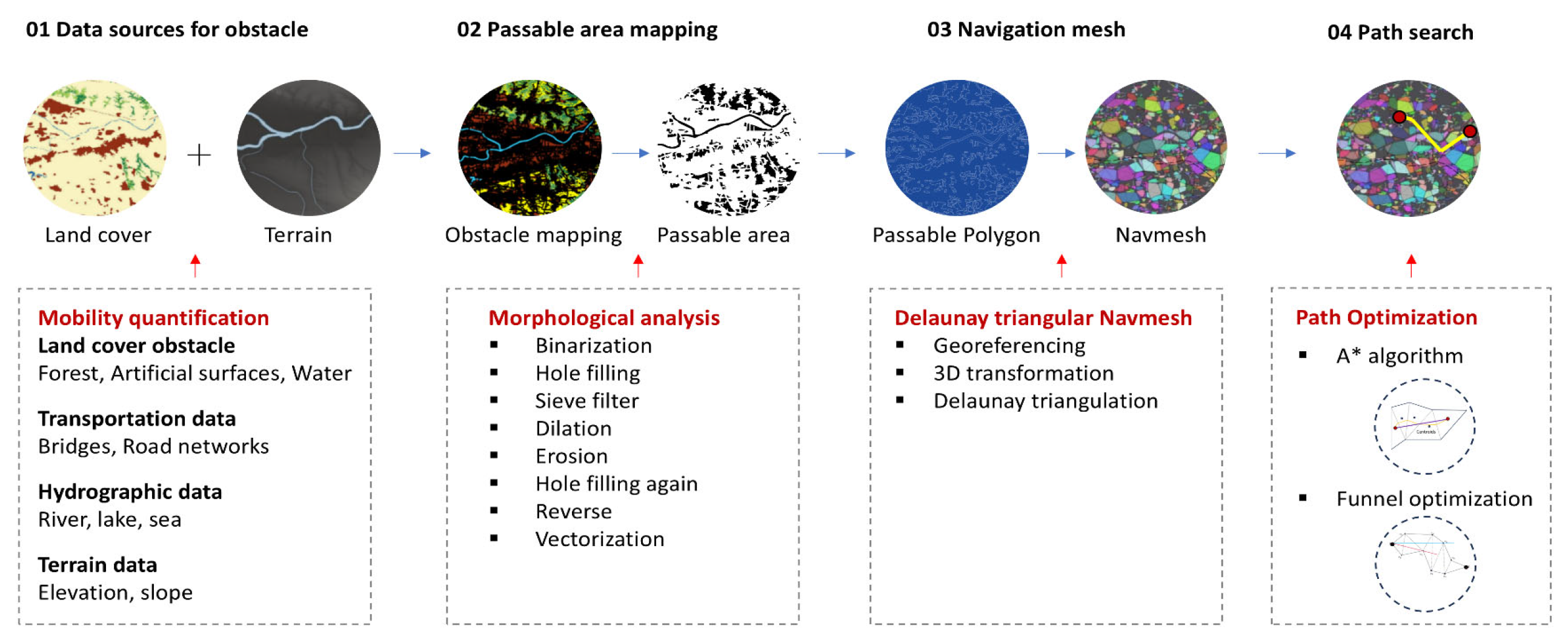
Off-road path planning often suffers from inefficiencies in data processing and high computational costs, particularly in dynamic terrains. An efficient path-planning algorithm that balances path quality, computational efficiency, and scalability while being adaptive to real-time environmental changes is still absent. To address the limitations, an improved off-road path-planning algorithm was developed in this study, as follows: (1) A land cover mobility model was introduced to facilitate generalizability at the national scale; (2) A Delaunay triangular NavMesh-based environment model was introduced to make efficient off-road environment representation; (3) An improved A* algorithm was introduced to derive efficient path planning in off-road environments.
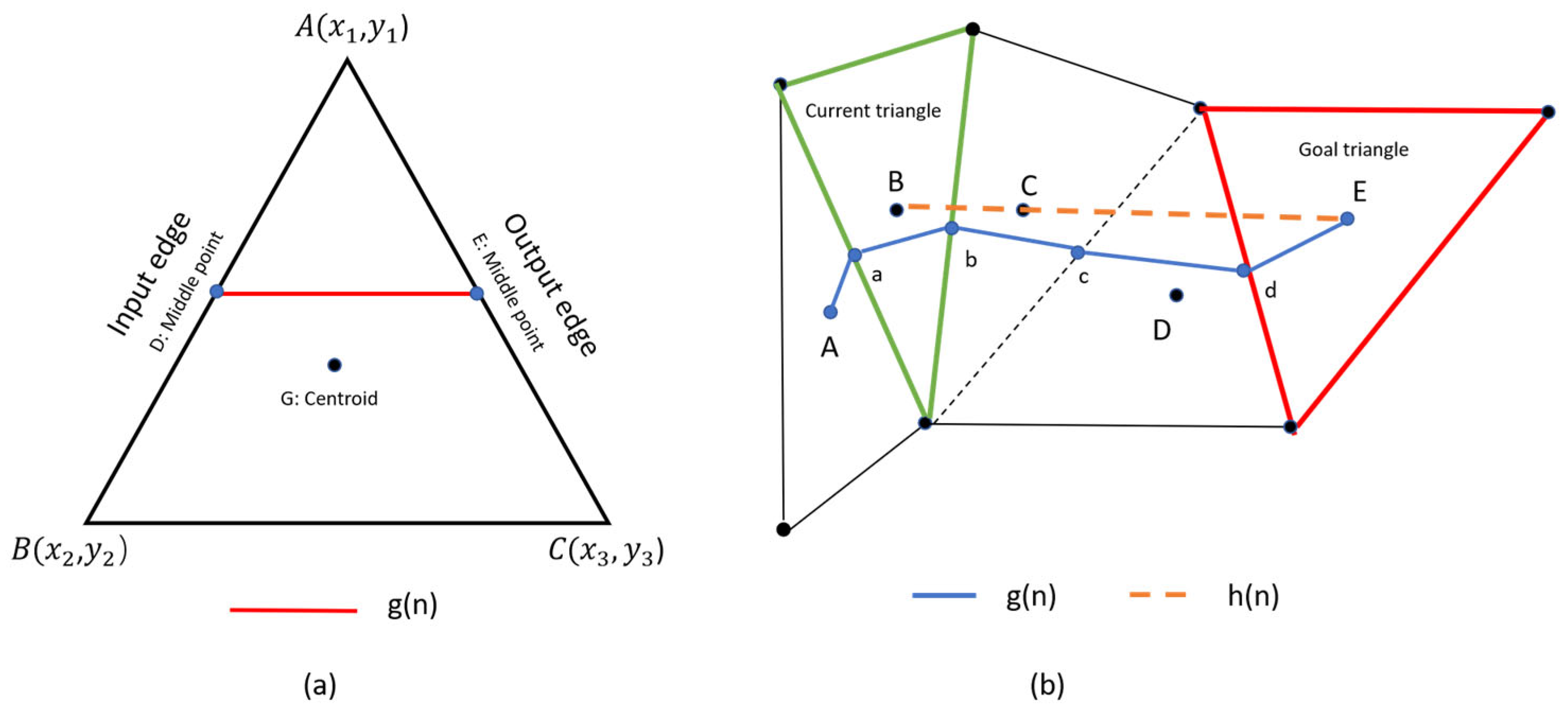
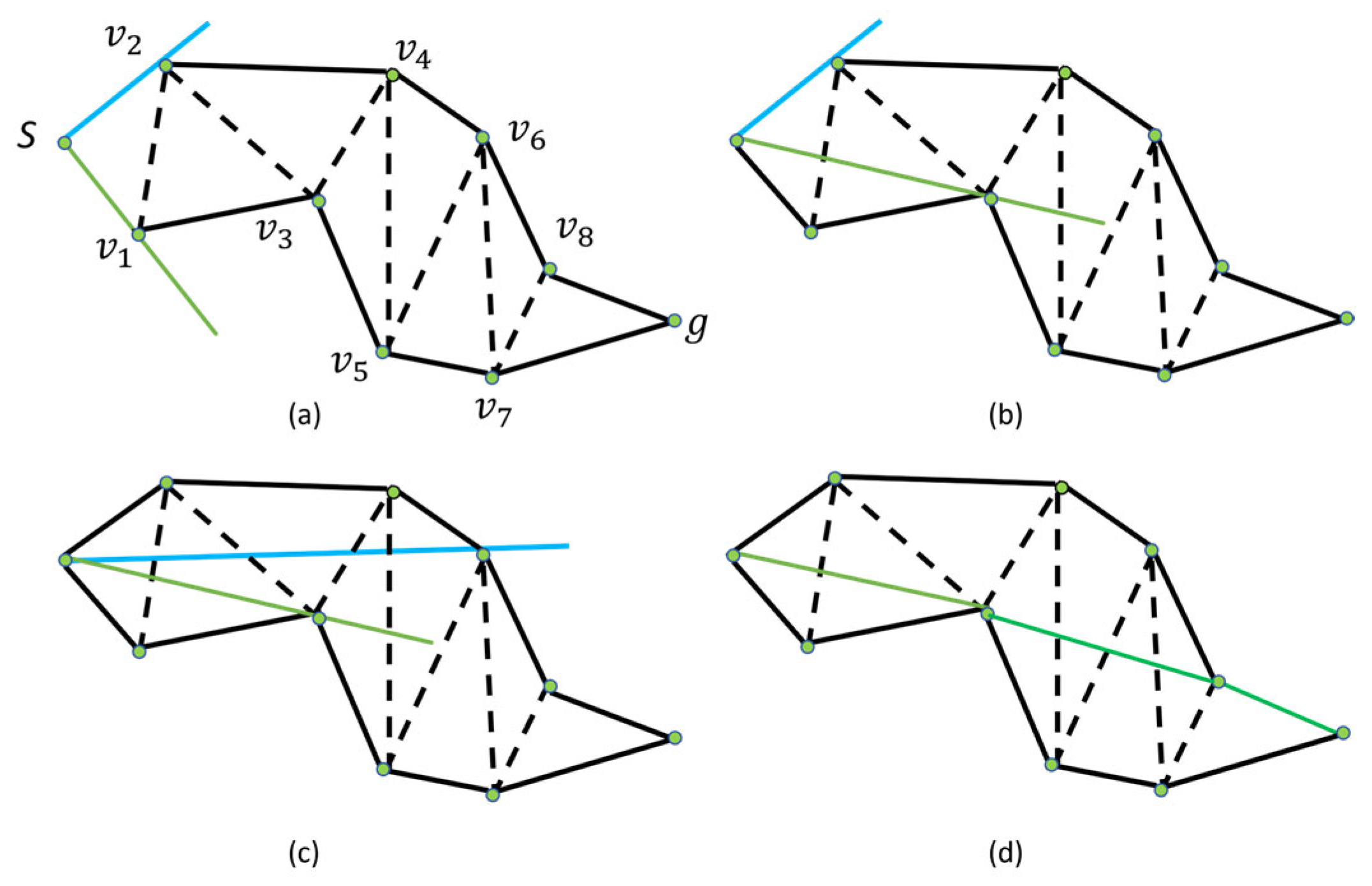
The key contribution of this study can be listed as below: (1) The paper innovatively integrates global-level LULC (land Use/land Cover) and DEM (Digital Elevation Model) datasets to model vehicle traversability in off-road environments, facilitating long-distance navigation at larger scales such as thousands of square kilometers (2). The paper innovatively adapts the Delaunay triangulation NavMesh model, an environment representation model commonly used in virtual gaming, to model real environments, which facilitates cost-effective off-road navigation. (3) The paper innovatively proposed an improved off-road path planning A* algorithm, based on the Delaunay triangulation navigation mesh, which uses the Euclidean distance between the midpoint of the input edge and the midpoint of the output edge as the cost function , and the Euclidean distance between the centroids of the current triangle and the goal as the heuristic function . The proposed algorithm will plan the optimized off-road mobility path from the start point to the end point, and determine a chain of path triangles that can be used to calculate the shortest path. (4) Given that the improved road-off path planning A* algorithm determines a chain of path triangles for calculating the shortest path, the funnel algorithm was then introduced to transform the path planning problem into a dynamic geometric problem, iteratively approximating the optimal path by maintaining an evolving funnel region, obtaining the shortest path closer to the Euclidean shortest path.
4. Discussion
The proposed framework includes innovations in both terrain-based mobility modeling and efficient environment representation. The following discussion elaborates on each component.
4.1. Off-Road Mobility Modeling and Environment Representation
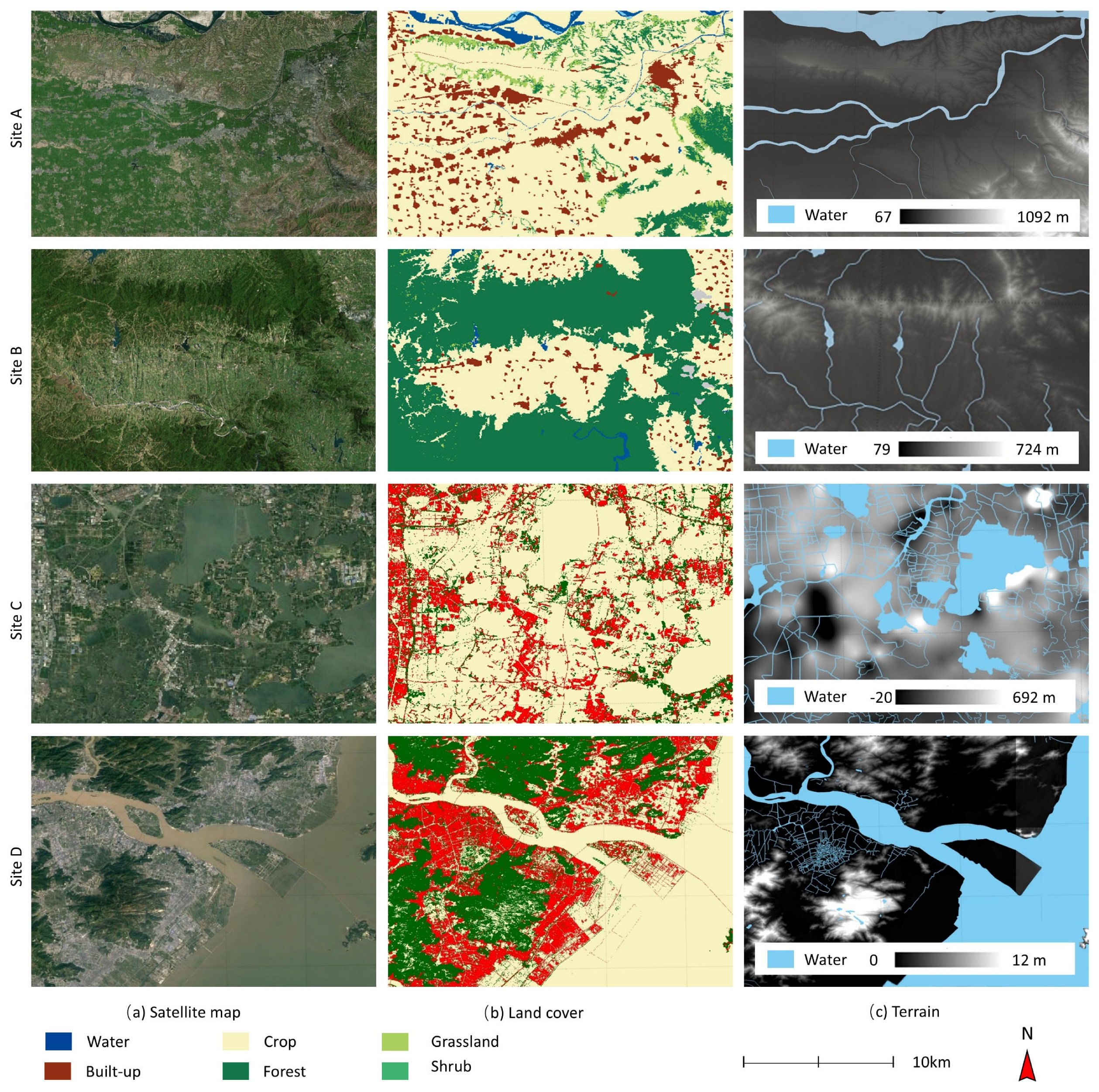
This study provides a new perspective and a uniform framework for quantifying off-road mobility modeling of geographic factors nationally. Off-road mobility assessments require the rapid identification of passable areas, necessitating an accurate quantitative analysis of the impact of regional geographic factors on vehicle performance. However, the significant variability in geographic environments, such as land cover and terrain features, across different regions makes it challenging to develop a universally applicable national mobility analysis model [
61]. This study addresses this challenge by leveraging the 30 m resolution land cover dataset of China, which includes both artificial built-up surface and vegetation cover data, in conjunction with publicly available global-scale DEMs. This integration enables a consistent classification standard, spatial-temporal resolution, coordinate system, and data accuracy for off-road mobility assessment across the entire China. This concept and method are consistent with studies indicating that a uniform classification baseline is necessary for application domains [
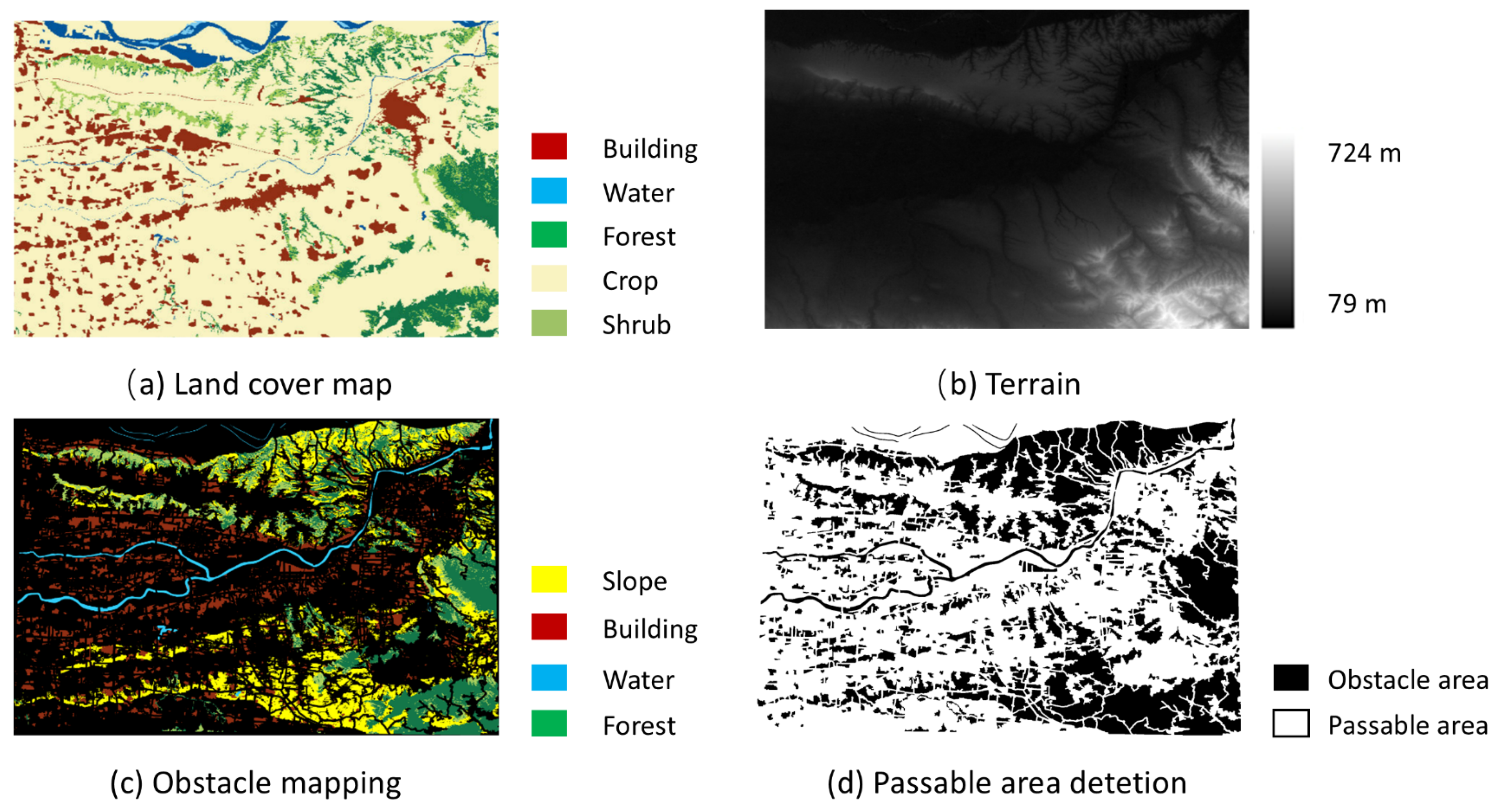
62], especially for navigation systems. In addition, due to the complex features and varied terrain in off-road environments, the obstacle regions generated inevitably exhibit irregularities such as boundary noise and internal holes, significantly impacting the accuracy and efficiency of subsequent path planning. Therefore, additional morphological analysis is necessary to refine the obstacle map to a cleaner and more precise passable map.
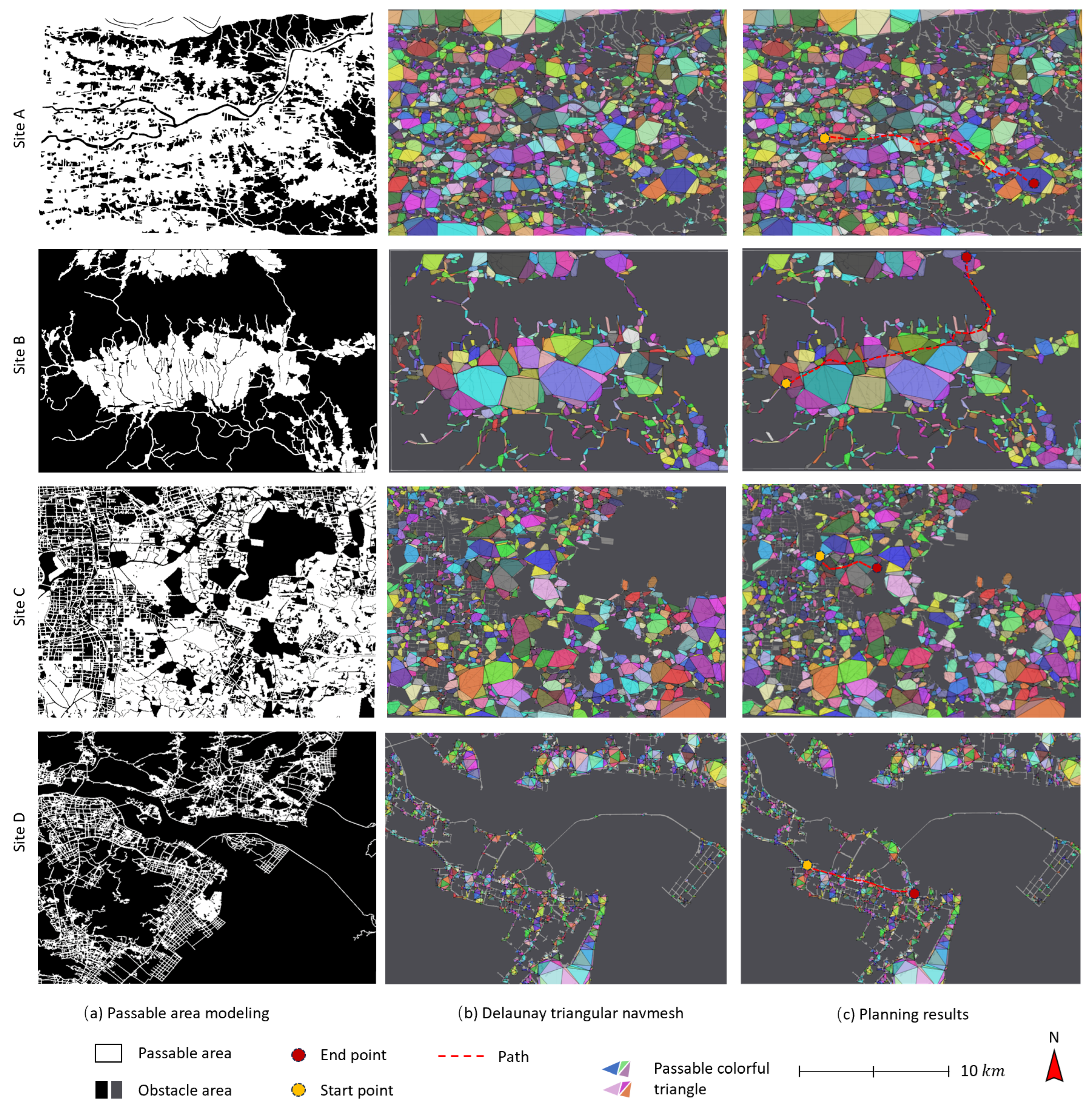
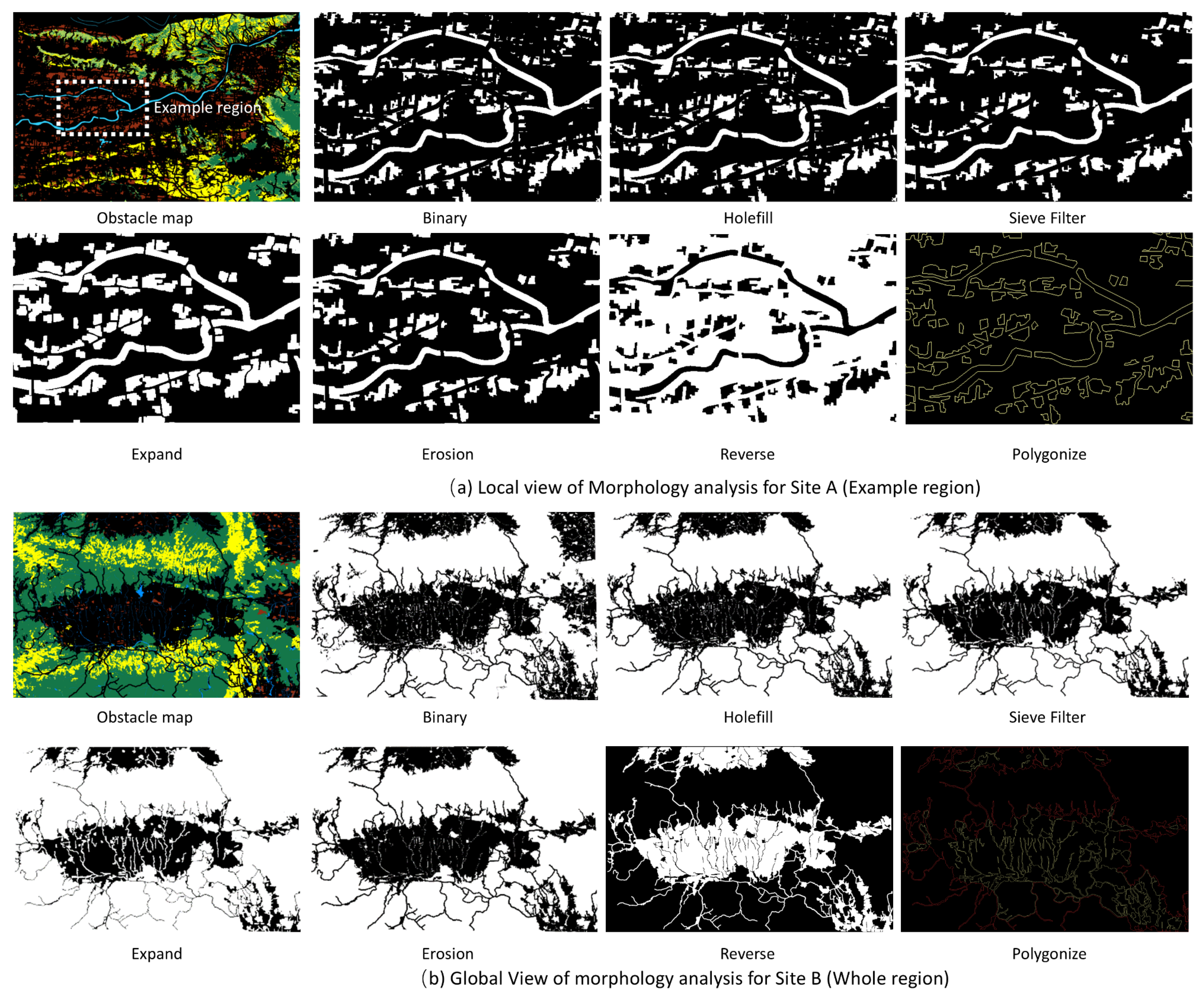
Figure 11 presents the obstacle distribution map generated for a specific region using the land cover and corresponding mobility parameters. White areas in (a–f) represent obstacles, while in (g) indicate passable regions. The obstacle regions in (b) appear fragmented and require mathematical morphology processing to form clean passable area mapping, consistent with demand in many public utility sectors where a cohesive and clean map is necessary for practical usage [
63]. The obstacle mapping framework with these morphological procedures not only facilitates a uniform classification standard for off-road environments but also ensures an efficient searching process for subsequent path planning.
The navigation mesh model proposed in this study facilitates efficient data loading and computational performance for path planning usage. In traditional grid-based path planning in off-road environments, where road networks are absent, the choice of grid size significantly impacts path planning efficiency [
64]. The characteristics of Delaunay triangulation are used to substantially reduce the number of triangular elements required to cover the target area, leading to fewer neighboring nodes loading. This technique mitigates the issue of excessive obstacle region expansion standards in regular grid-based methods, as the Delaunay triangulation dynamically adjusts triangle sizes to conform to the shape of obstacles [
65]. The number of polygons, including units or triangles, was used to assess the data efficiency of the navigation meshes compared to other path-planning database types. This can be proved by
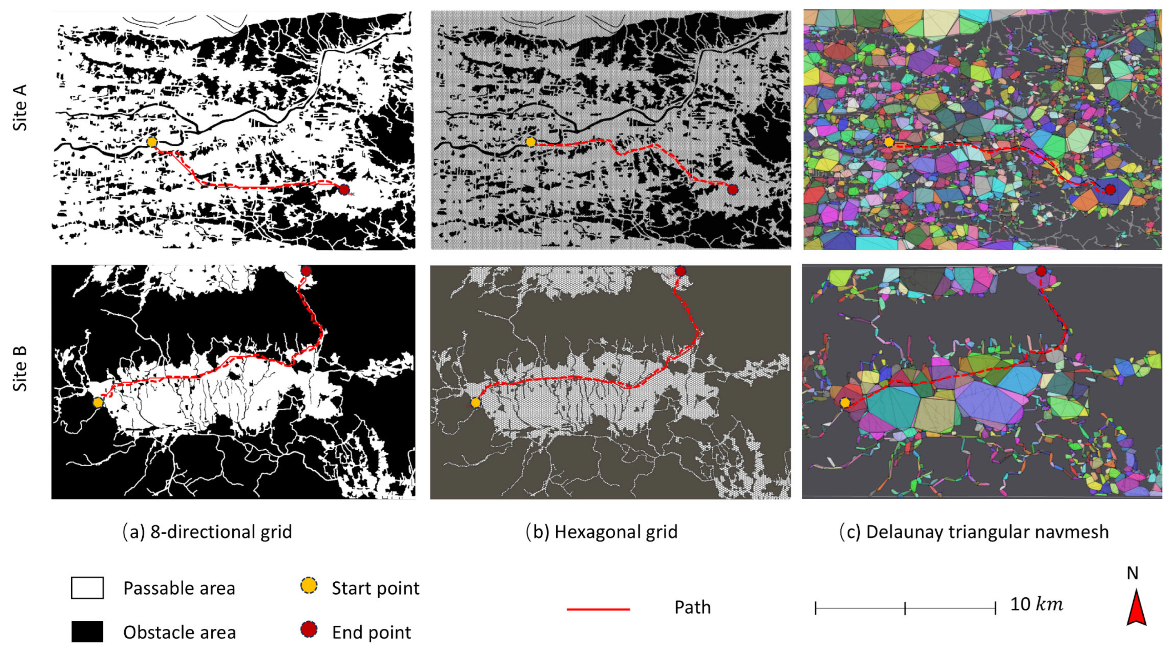
Table 7, which indicates that the navigation meshes yielded significantly fewer units than the 8-directional grids and hexagonal grids. As depicted in
Table 7, the grid cell counts in 8-directional, hexagonal, and navigation mesh grids are determined by the underlying geometric structures: pixel cells, hexagonal cells, and triangles, respectively. In site A, the navigation mesh produced 10,523 units, which is only 21.2% of the units of hexagonal grids and 0.6% of the units of 8-directional grids. In site B, the navigation mesh produced 5120 units, which is only 56.7% of the units of the hexagonal grids and less than 1% of the 8-directional grids. Although Site A is clearly far more complex than Site B, as indicated by the number of units in 8-directional grids and hexagonal grids (with a ratio of 2.49 to 5.49 times more complex), the navigation mesh yielded significantly simpler units in both sites (with a ratio of 2.1 times more complex), further proving that navigation meshes can produce simple and concise navigation systems. By eliminating unnecessary obstacle data in large, unobstructed areas, this approach significantly reduces the number of triangles and neighboring nodes to be explored during path planning. This reduction not only simplifies the search process but also improves computational efficiency, a critical factor in real-time applications for autonomous vehicles operating in off-road environments.
According to the previous research [
66,
67], the time complexity of the Navmesh is
, while the time complexity of the grid is
. Here,
represents the number of polygons in the navigation mesh, and
represents the grids in a map. As can be seen from
Table 7,
. Therefore, the complexity of the Navmesh is much lower than the computational complexity of the grid. This also theoretically proves that the proposed algorithm in this article has high efficiency in path planning compared with grid-based methods.
The proposed optimized A* algorithm, coupled with a funnel algorithm, yields significantly shorter paths and improved computational efficiency compared to conventional methods. Traditionally, path planning algorithms in continuous spaces require paths to traverse through the midpoints of shared edges in a triangle path chain. However, this constraint often leads to sub-optimal solutions, particularly in navigation mesh-based path planning. To address this limitation, the proposed algorithm leverages the navigation mesh structure and employs a novel cost function based on the distance between the midpoints of shared edges in the path chain. Additionally, a heuristic function, utilizing the distance between the triangle centroid and the goal, guides the path search process. To further refine the generated paths, a funnel algorithm is integrated. Extensive experiments conducted in diverse off-road environments demonstrate that the algorithm consistently produces shorter paths and significantly outperforms conventional methods in terms of computational efficiency. This improvement is primarily attributed to the inherent advantages of navigation mesh-based path planning, which allows for efficient exploration of the searching space within triangular regions, eliminating the need for exhaustive cell-by-cell traversal and searching in conventional grid-based searching algorithms. Thus, the algorithm can quickly identify sub-optimal solutions, thereby meeting the stringent timing requirements of real-time path planning applications. The experimental results demonstrate the superiority of the proposed algorithm in terms of path quality and computational efficiency for off-road scenarios.
To verify the effect of the funnel algorithm, an ablation experiment is conducted; results are shown in
Table 8 and
Figure 12.
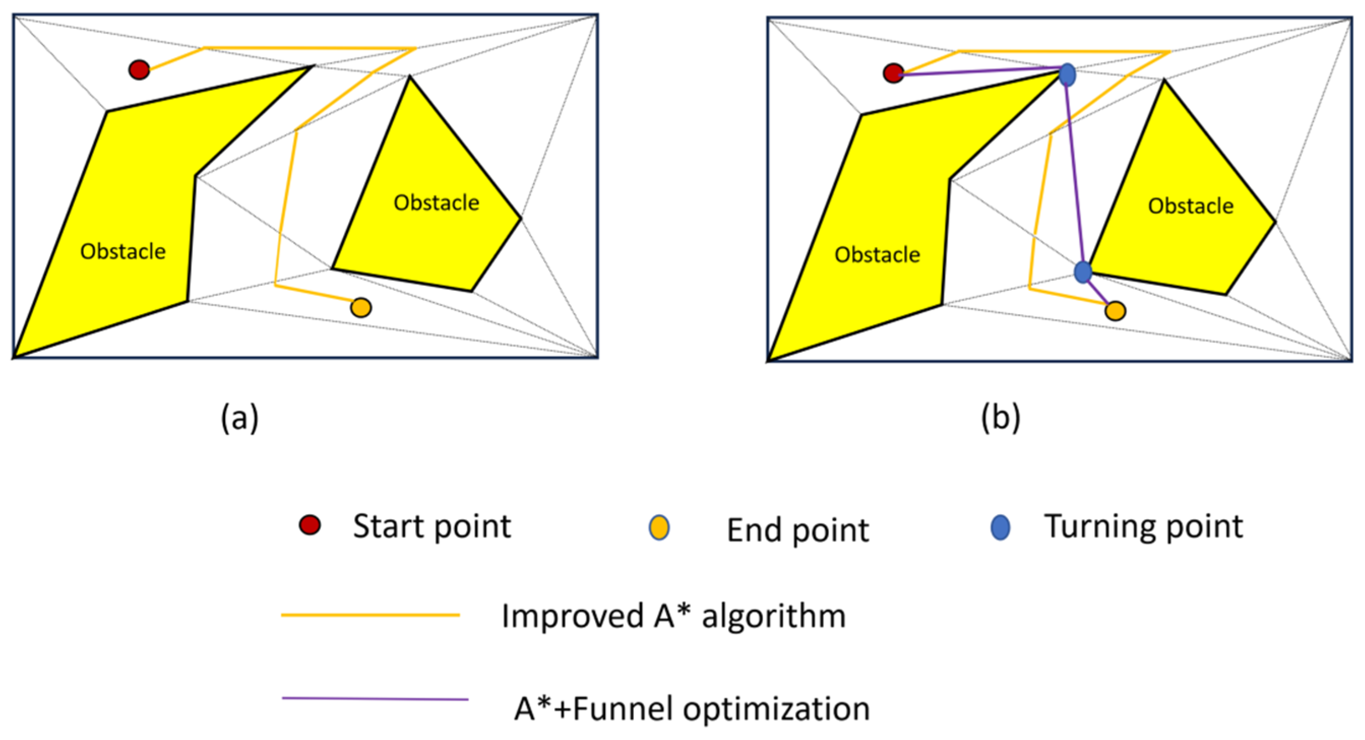
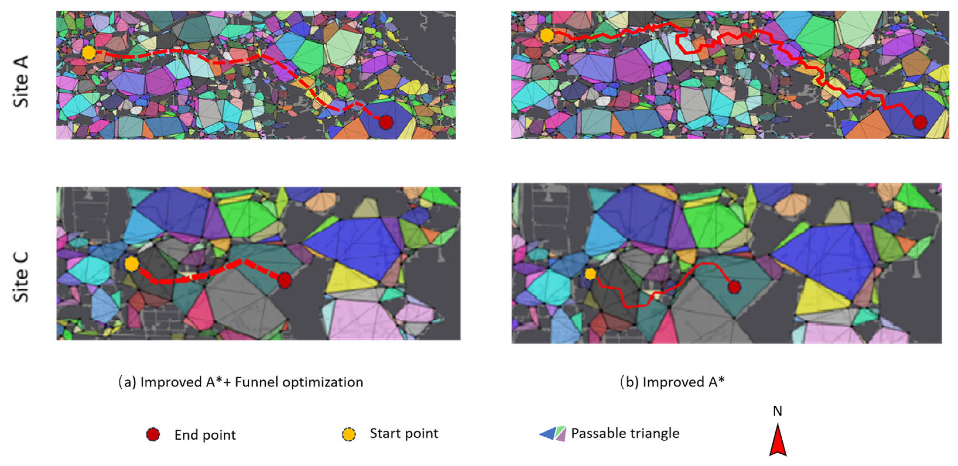
From
Figure 12, it could be seen that the path obtained by the improved A* algorithm on navigation meshes is relatively rugged and does not necessarily correspond to the Euclidean shortest path. In contrast, the improved A* path planning algorithm optimized by the funnel algorithm outperformed the improved A* algorithm, achieving much distance savings in total path distance.
Table 8 demonstrates that although the funnel algorithm can prolong the running time by about 1~5%, the path obtained is significantly shorter than the improved A* algorithm.
4.2. Structural and Algorithm Efficiency Validation Through Comparative Experiment
To further demonstrate the structural and algorithmic advantage of the proposed Delaunay triangular NavMesh and improved A*+Funnel optimization, a supplementary comparison was conducted using the well-established Dijkstra algorithm.
Table 9 shows the path length and computation time for both structures using Dijkstra. It can be seen that the NavMesh model produced a slightly longer path (2.61 km vs. 2.74 km), but the computation time was drastically lower—only 5 ms, compared to 3430 ms under the grid model. This illustrates that even under identical search logic, the NavMesh achieves superior computational efficiency by reducing the number of nodes and avoiding unnecessary expansions. This substantial speedup is attributed to the adaptive and sparse triangulation of the NavMesh. Unlike fixed-size grids that generate uniform dense nodes—regardless of terrain complexity—the NavMesh dynamically adjusts triangle sizes, using large triangles in open areas and smaller ones near obstacles. This significantly reduces the number of searchable units and accelerates node expansion.
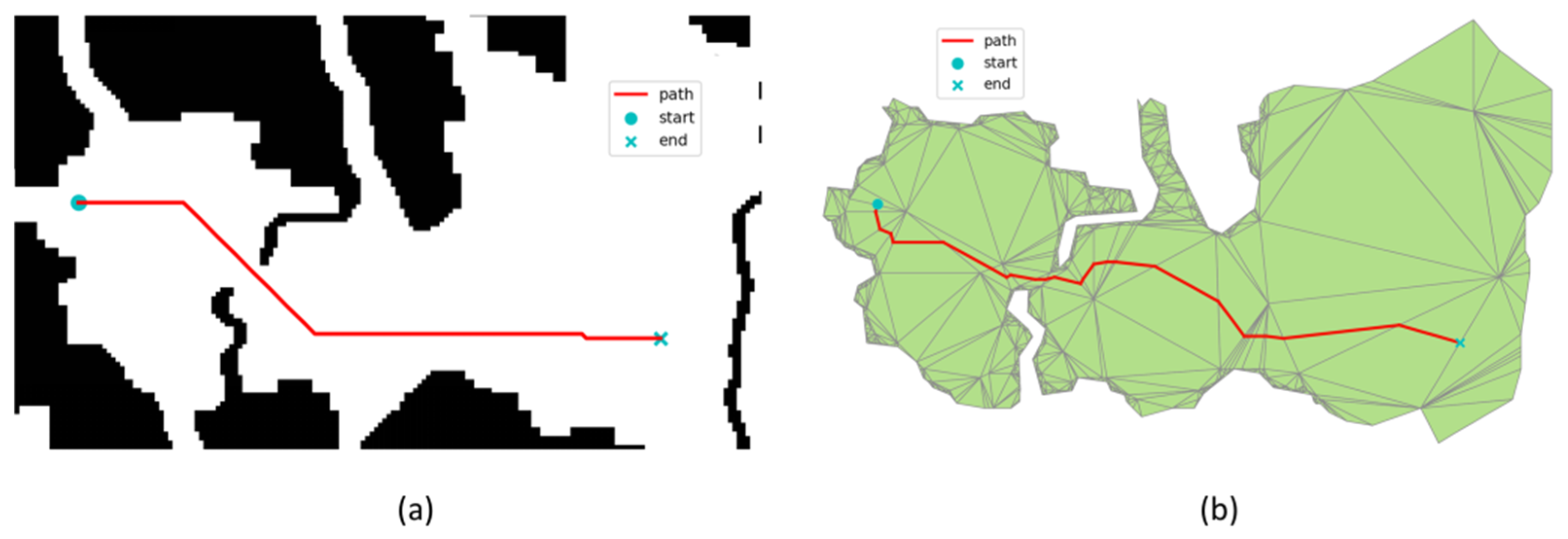
Figure 13 further illustrates this structural difference. In
Figure 13a, the path over the grid appears rigid and inefficient due to fixed cell directions. In contrast,
Figure 13b shows how the NavMesh structure enables smoother and more realistic traversal, tightly conforming to passable regions without redundant detours. Additionally,
Table 10 presents the experimental results of different algorithms applied to the NavMesh. Both Dijkstra and A* algorithms yield the same shortest path, which corresponds to the result shown in
Figure 13b, and thus is not repeated here; the red path in
Figure 13b indicates the Dijkstra and A* algorithms. The only difference lies in the computation time: A* achieves a shorter runtime—1 millisecond, compared to 5 milliseconds for Dijkstra. This further demonstrates the effectiveness of the NavMesh model proposed in this study.
These results collectively support a key insight: that efficient off-road path planning does not solely rely on the complexity of the search algorithm, but significantly benefits from the underlying environmental representation. By leveraging the structural flexibility of Delaunay triangulation, our NavMesh model inherently reduces node complexity and enables faster, smoother path computation. This structural advantage remains evident across both heuristic-based (A*) and non-heuristic (Dijkstra) algorithms, underscoring its robustness and generalizability.
In order to further prove the efficiency of the proposed algorithm, the proposed improved A*+Funnel optimization algorithm is compared with the Dijkstra algorithm in Sites (a) and (b). The results in
Figure 14 further illustrate the differences between the two algorithms. The algorithm proposed in this paper realizes a smoother path. On the contrary, the paths generated by the Dijkstra algorithm are more redundant.
Table 11 shows the experimental results of different algorithms applied to Navmesh. Compared with the Dijkstra algorithm, the algorithm proposed in this paper can produce the shortest path, which corresponds to the blue line shown in
Figure 14. Compared with Dijkstra’s 8 milliseconds, the proposed algorithm only needs 2 milliseconds. Additionally, the path length planned by the algorithm proposed in this paper has been shortened by nearly half compared with the Dijkstra algorithm (2.95 km vs. 4.85 km), which further proves the effectiveness of the proposed algorithm.
4.3. Advantages, Limitations, and Recommendations
This study introduces a novel off-road path planning algorithm utilizing a navigation mesh model to model the complex off-road environments using Delaunay triangulation. The method was established in a database concentrating on a national scale, in which its effectiveness was proved by 4 cases with typical natural and social landscapes. While the proposed off-road path planning algorithm significantly increases accuracy and efficiency, there are still some limitations. Firstly, the current mobility assessment is based on a binary classification of passable and non-passable areas, failing to adequately take into consideration the continuous and multi-layered nature of geographic environments. Real-world terrain generally exhibits a continuous spectrum of mobility influenced by multiple geographical conditions and the mobility parameters of the vehicles. Secondly, it is difficult to precisely characterize particular topographic features in various regions due to the land cover data used in this study’s weak classification accuracy at small scales. These mapping products, while providing a generalized global classification for China, are limited by the complexity of global geographic environments and lack the granularity to represent regional variations accurately. In addition, the proposed approach does not account for vehicle dynamic constraints, which can affect the realism and safety of the generated paths.
In the future, the research could incorporate multi-scale terrain analysis, soil types, vegetation cover, and vehicle factors to capture the interactive effects of various geographic elements on vehicle mobility, thereby establishing a more refined mobility model and further enhancing the algorithm’s feasibility and applicability. Furthermore, the subsequent research could integrate high-resolution remote sensing imagery and field survey data to construct more region-specific land cover classification systems, thereby improving path planning accuracy. Future research should consider vehicle dynamic constraints to develop more realistic path planning models. Additionally, multi-objective path planning, which simultaneously considers factors such as path length, energy consumption, and safety, represents an important direction for future exploration. This optimization achieved in off-road path planning has the potential for a wide range of similar applications, including autonomous vehicle navigation in rugged terrains [
6,
20] and virtual nuclear facility simulations, where precise path planning is essential to minimize exposure [
61].
5. Conclusions
This study introduces a novel off-road path planning algorithm that utilizes a navigation mesh model and an optimized A* algorithm, effectively modeling complex off-road environments using Delaunay triangulation and obstacle constraints in a compact database. The A* search algorithm, enhanced with a funnel algorithm, is employed to efficiently find optimal paths within the navigation mesh. Experimental results show that this method significantly outperforms grid-based approaches, achieving a 5% to 20% reduction in total path distance and a planning time of 150 to 170 milliseconds, which is significantly faster than the conventional 8-directional and hexagonal grid method, indicating a substantial improvement in computational efficiency. The navigation mesh requires less than 1% of the original data volume, highlighting its computational efficiency and potential applications in enhancing off-road vehicle capabilities and aiding disaster response operations. By employing a navigation mesh, the algorithm successfully captures intricate terrain details. The profound impacts of the algorithm proposed in this paper can be summarized as follows: (1) Using Delaunay Navmesh achieves environmental modeling of passable areas with only 1% of the data compared with grid-based methods, which demonstrates its high data-model efficiency; (2) The algorithm proposed in this paper can obtain the shortest path and effectively support decision-making in path planning.
Nonetheless, limitations remain, including a binary representation of terrain traversability, simplistic land cover classification, and a lack of consideration for vehicle kinematics. To address these, future work should focus on enhancing the environmental representation by integrating high-resolution land cover maps, vehicle dynamic models, and elevation-based terrain detail. Moreover, with the increasing availability of high-frequency remote sensing imagery and geospatial big data, there is significant potential to adapt this framework for near-real-time, large-scale operations. Incorporating temporally dynamic and data-driven terrain assessments will further enhance the robustness and adaptability of the algorithm, particularly in rapidly changing conditions such as natural disasters or extreme weather events.


