A Semi-Active Control Method for Trains Based on Fuzzy Rules of Non-Stationary Wind Fields

Abstract

The stochastic fluctuation characteristics of wind speed can significantly affect the control performance of train suspension systems. To enhance the running quality of trains in non-stationary wind fields, this paper proposes a semi-active control method for trains based on fuzzy rules of non-stationary wind fields. Firstly, a dynamic model of the train and suspension system was established based on the CRH2 (China Railway High-Speed 2) high-speed train and magnetorheological dampers. Then, using frequency–time transformation technology, the non-stationary wind load excitation and train response patterns under 36 common operating conditions were calculated. Finally, by analyzing the response patterns of the train under different operating conditions, a comprehensive control rule table for the semi-active suspension system of the train under non-stationary wind fields was established, and a fuzzy controller suitable for non-stationary wind fields was designed. To verify the effectiveness of the proposed method, the running smoothness of the train was analyzed using a train-semi-active suspension system co-simulation model based on real wind speed data from the Lanzhou–Xinjiang railway line. The results demonstrate that the proposed method significantly improves the running quality of the train. Specifically, when the wind speed reaches 20 m/s and the train speed reaches 200 km/h, the lateral Sperling index is increased by 46.4% compared to the optimal standard index, and the vertical Sperling index is increased by 71.6% compared to the optimal standard index.

1. Introduction

Strong wind conditions can severely deteriorate the dynamic performance of trains. With the continuous increase in train operating speeds, this impact is becoming more pronounced [1]. Currently, railway authorities primarily ensure the safety of train operations in strong wind environments through measures such as controlling train speeds [2], constructing windbreak walls [3], and optimizing the aerodynamic structures of trains [4]. In addition, to further enhance the running quality of trains under complex operating conditions and to meet passengers’ demands for comfort, railway authorities have set higher requirements for train running smoothness [5]. Against this backdrop, an increasing number of scholars are working to improve the dynamic performance of trains by optimizing the suspension systems, thereby enhancing train running smoothness [6].

Common control methods for suspension systems include PID control, linear optimal control, H∞ control, neural network control, and fuzzy control [7,8,9]. Among these, fuzzy control does not depend on precise mathematical models and has strong adaptability to nonlinear systems and stochastic disturbances. It is often used in semi-active suspension systems subjected to random excitations. For example, for the semi-active suspension system with magnetorheological dampers, Ma Xinna et al. [10] proposed an adaptive fuzzy control method. Experimental results show that this method not only suppresses electromagnetic interference but also effectively improves the dynamic performance of the suspension system. Yin Zongjun et al. [11] developed a fuzzy PID controller based on an 8-DoF active suspension model. Comparative experiments with passive suspension systems and conventional PID controllers demonstrated the superior performance of the proposed control method. Li Hongyi et al. [12] proposed an adaptive event-triggered fuzzy control method based on Lyapunov stability theory. This method also takes into account the problem of actuator failures, thereby enhancing the practicality of the suspension system. Liu Yongming et al. [13], based on an adaptive backstepping technique along with specific Lyapunov functions, proposed an adaptive fuzzy output feedback fault-tolerant control method and applied it to the active suspension system. Meanwhile, by employing parameter estimation techniques, a fault compensation strategy has been developed, thereby eliminating the need for knowing efficiency indexes. In summary, scholars have conducted extensive research on fuzzy control methods for suspension systems and have demonstrated the practicality and effectiveness of these methods in suspension systems. However, this control method is highly dependent on historical experience, and therefore, it may not achieve the desired control effect in practical applications.

To address this issue, we analyzed the time–domain characteristics of gusty winds and the instability patterns of trains under stochastic wind fields based on real wind speed data along the railway line. We then established fuzzy control rules for train suspension systems in non-stationary wind field environments. In addition, train suspension systems mainly consist of passive suspension, active suspension, and semi-active suspension [8]. The semi-active suspension system can significantly improve the running smoothness of trains and passenger comfort by adjusting the damping force in real time to change the overall stiffness of the suspension [14]. Moreover, the semi-active suspension system has the advantages of low energy consumption, low cost, fast response, easy improvement, and strong adaptability to complex operating conditions [15]. Therefore, this paper proposes a semi-active control method for trains based on fuzzy rules of non-stationary wind fields, targeting the semi-active suspension system.

The specific contributions and innovations are as follows:

• A semi-active control method for trains in non-stationary wind field environments is proposed. This method effectively optimizes the dynamic performance of trains under non-stationary wind conditions and thereby enhances train running smoothness by real-time adjustment of the variable damping force of the semi-active suspension system.
• The instability characteristics of trains in stochastic wind fields are analyzed using harmonic synthesis methods and dynamic simulation techniques, and fuzzy control rules for train suspension systems suitable for non-stationary wind field environments are established.
• A real wind speed dataset from the Lanzhou–Xinjiang railway line is collected to verify the performance of the proposed method.

2. Dynamics Model of the Train and Suspension System

2.1. Simplified Model of the Train

This paper is conducted against the background of practical engineering applications on the Lanzhou–Xinjiang railway line. Therefore, we established a simplified whole-vehicle model based on the CRH2 train operating on the Lanzhou–Xinjiang line. As shown in Figure 1, the simplified whole-vehicle model consists of three rigid bodies: the car body, the bogie frame, and the wheelset. These rigid bodies are connected by elastic elements. The expression for the train dynamics model is as follows [16].

$$M\ddot{X}+C\dot{X}+KX=F_m$$

(1)

where M, C, and K represent the mass matrix, damping matrix, and stiffness matrix of the train system, respectively. X represent the displacement response of the train system. F_m denotes the generalized vector of external excitation. The subsequent research mainly focuses on external wind load excitation.

In Figure 1, m_C, m_F, m_W represent the mass of the car body, the bogie frame, and the wheelset, respectively. ki and ci represent the elastic coefficients and damping coefficients of each part, respectively.

2.2. Dynamics Model of the Semi-Active Suspension System

In the previous section, a simplified model of the train system was established, where the suspension system is a passive suspension system with springs and dampers connected in parallel. However, the passive suspension system has a fixed elastic coefficient, and its suspension characteristics cannot be adaptively adjusted according to external excitations, which limits the improvement of the train’s dynamic performance [7]. To further optimize the dynamic performance of the train under strong wind conditions and enhance the train’s running quality, this paper introduces a magnetorheological damper, which has strong stability, fast response, high control accuracy, and large output damping force, into the suspension system in parallel to establish a semi-active suspension system with a variable damper [10]. The magnetorheological damping force can be expressed as:

$$F_{MD}=c_i{\dot{x}}_i+C_{MD}$$

(2)

where c_i denotes the damping coefficient of the inherent damping, x_i represents the relative displacement at the installation point of the variable damper, and C_MD represents the variable damping force of the magnetorheological damper. After incorporating it into the suspension system, the dynamic model is as follows.

$$M\ddot{X}+C\dot{X}+C_{MD}+KX=F_m$$

(3)

3. Response Patterns of Trains Under Non-Stationary Wind Loads

3.1. Simulation of the Non-Stationary Wind Loads

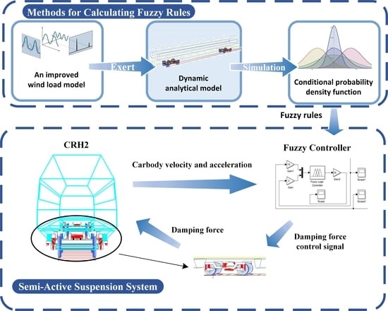
3.1.1. Simulation of Random Gust Wind

To calculate the non-stationary wind loads, we first simulated the random gust wind field. In this paper, the gust wind speed is simulated based on the wind speed power spectrum. The commonly used Davenport wind speed power spectrum is constructed based on the wind speed at the standard height, which is not entirely consistent with the actual operating height of the train. Therefore, this paper adopts the Kaimal spectrum provided by the international electrotechnical commission. The expression for the power spectrum is as follows:

$$S_u(z,f)={\displaystyle \frac{4L{\sigma }^2}{U\left(z\right){\left(1+6f_L\right)}^{5/3}}},f_L={\displaystyle \frac{fL}{U\left(z\right)}}$$

(4)

where S_u represents the single-sided spectrum of the lateral component, z denotes the height, σ and L represent the standard deviation and the turbulence integral scale, respectively, and f_L represents the reduced frequency. The values for the above parameters are referenced from the literature [5]. f is the frequency, and U(z) represents the mean wind speed at height z. Since wind speeds are typically measured at the standard height along the railway line, it is necessary to introduce a function for the variation of wind speed with height [17]:

$$U_Z={\displaystyle \frac{\lg z-\lg z_0}{\lg z_s-\lg z_0}}U(z_s)$$

(5)

where z₀ represents the height at which the wind speed decreases to zero, and z_s represents the standard height. Here, the Lanzhou–Xinjiang Railway is taken as an example for study [18]. The values are set as z₀ = 0.05 m, z_s = 10 m.

There is a certain correlation between wind speeds [19]. When a train passes through a crosswind area, the leading car, intermediate cars, and tail car are simultaneously disturbed by the turbulent wind field. Therefore, the influence of this correlation needs to be considered. In the gust wind field, this correlation is commonly expressed mathematically using the coherence function of gust wind. Since the length-to-height ratio of the train is relatively large, the wind speed measurement points on the train surface can be regarded as a one-dimensional distribution. Let the number of measurement points be n, and the spacing between measurement points be ∆. By substituting the commonly used coherence functions of Davenport and Shiotami, for any two measurement points v_j and v_m, the expressions for the two coherence functions are as follows:

Davenport coherence function:

$$co{h}_v(v_j,v_m)={\left. [\exp \left(-c_v{\displaystyle \frac{\Delta \cdot f}{U_z}}\right)\right]}^{\left|j-m\right|}$$

(6)

Shiotami coherence function:

$$co{h}_v(v_j,v_m)={\left. [\exp \left(-{\displaystyle \frac{\Delta }{L}}\right)\right]}^{\left|j-m\right|}$$

(7)

where c_v is the exponential decay coefficient, and L represents the turbulent integral scale.

Combining the two coherence functions, the expression for the random wind speed time history χ_u at the j-th simulation point is as follows [20].

$$\begin{array}{l}{\chi }_u(p\Delta t)=\mathrm{Re}\left\{{\displaystyle \sum _{m=1}^j{h}_{jm}(q\Delta t)\exp \left. [i\left(\frac{m}{n}\Delta \omega \right)p\Delta t\right]}\right\}\\ (j=1,2,\dots ,n), (p=0,1,\dots ,M\times n-1)\end{array}$$

(8)

where ∆t represents the sampling interval time, i = $\sqrt{-1}$, M = 2N, N is the number of sampling frequency points, and ∆ω is the frequency increment, where ∆ω = ω/N.

The Fast Fourier Transform (FFT) technique is introduced to calculate h_jm(p∆t), and its expression is as follows.

$$h_{jm}\left(q\Delta t\right)={\displaystyle \sum _{l=0}^{M-1}{B}_{jm}(l·\Delta \omega })\exp \left. [i\left(l\Delta \omega \right)\left(q\Delta t\right)\right]$$

(9)

where B_jm(l∆ω) is as follows:

$$\begin{array}{l}{B}_{jm}\left(l\Delta \omega \right)=\left\{\begin{array}{cc}\begin{array}{l}\sqrt{2\left(\Delta \omega \right)}{H}_{jm}\left(l\Delta \omega +{\displaystyle \frac{m\Delta \omega }{n}}\right)\exp \left(i{\phi }_{ml}\right),\end{array}& 0\le l<N\\ 0,& N\le l\le M-1\end{array}\right.\\ \begin{array}{ccc}& & \end{array}\left(l=0,1,2,\dots ,M-1\right)\end{array}$$

(10)

In the equation, φ_ml is the uniformly distributed random phase angle within [0, 2π].

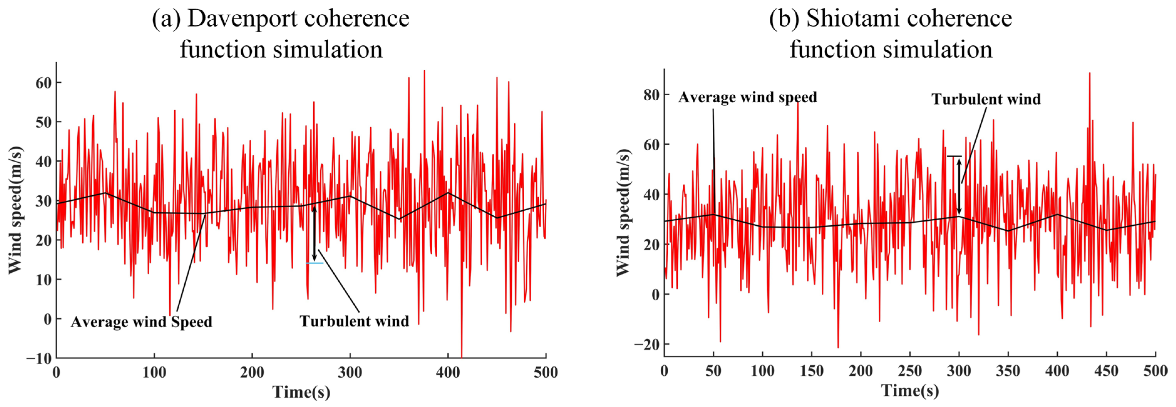
Based on the above formula, the simulated gust wind speed time history is shown in Figure 2. The mean wind speed data in Figure 2 are derived from the actual wind speed measurements collected along the Lanzhou–Xinjiang railway line.

Based on the actual wind speed measurement results, it can be found that the maximum instantaneous wind speed in this area does not exceed 60 m/s. Therefore, by comparing the simulated gust wind speed results in Figure 2, it can be seen that the wind speed time history calculation results based on the Davenport coherence function are more accurate.

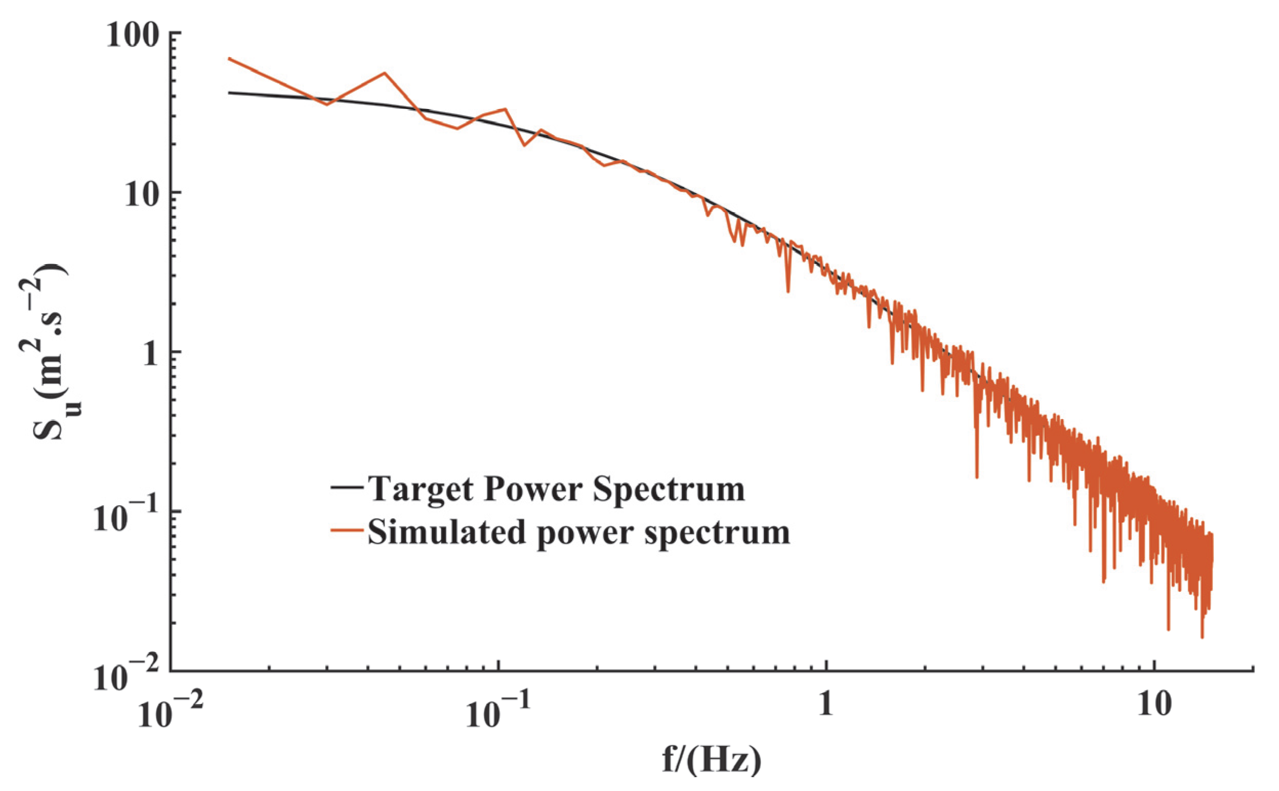
According to the gust wind time history calculation results in Figure 2, the simulated wind power spectrum is shown in Figure 3.

Based on the comparison of the wind speed power spectrum fitting degree in Figure 3, it is found that the wind speed simulation spectrum based on the Davenport coherence function matches the target wind speed power spectrum well, which proves the validity of the simulation results [21].

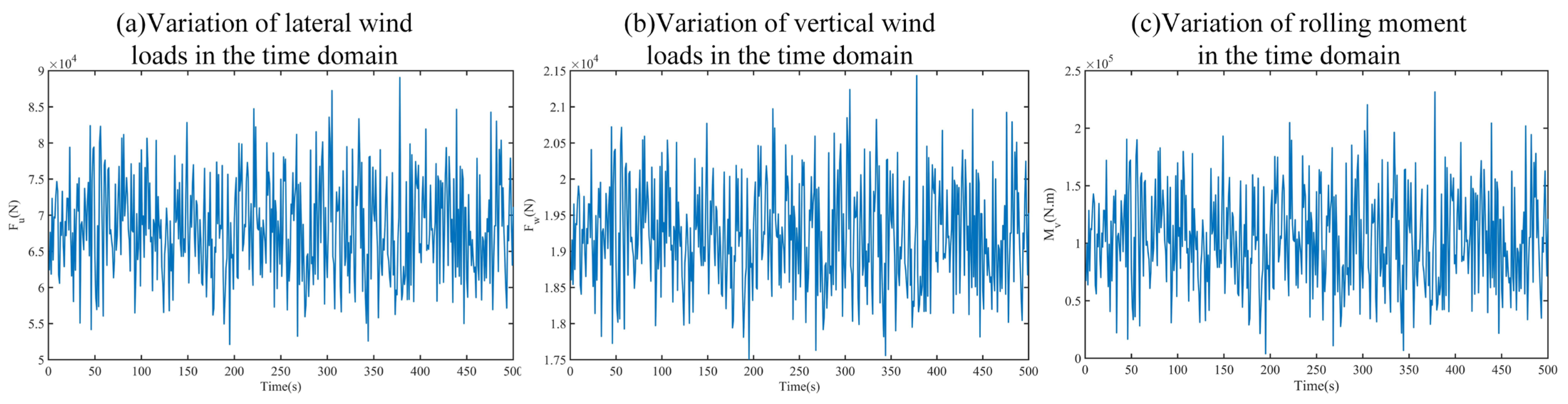
3.1.2. Calculation of Non-Stationary Wind Loads

Non-stationary wind loads mainly include the static wind force caused by the mean wind and the buffeting wind force caused by gusty wind. The static wind force on the surface of the train body is as follows [22].

$$F^{st}=\left\{\begin{array}{c}{F}_u^{st}={\displaystyle \frac{1}{2}}\rho A\left({\left(U_Z\cos \beta +V\right)}^2+{\left(U_Z\sin \beta \right)}^2\right)C_u(\psi )\\ F_w^{st}={\displaystyle \frac{1}{2}}\rho A\left({\left(U_Z\cos \beta +V\right)}^2+{\left(U_Z\sin \beta \right)}^2\right)C_w(\psi )\\ M_v^{st}={\displaystyle \frac{1}{2}}\rho A\left({\left(U_Z\cos \beta +V\right)}^2+{\left(U_Z\sin \beta \right)}^2\right)H{C}_{Mv}(\psi )\end{array}\right.$$

(11)

In the equation, the equivalent static wind force F^st acting on the train surface includes lateral force, vertical force, and rolling moment; u, w, and v represent the lateral, vertical, and longitudinal directions, respectively; ρ is the air density; A is the frontal area of the train body, V represents the train speed, β is the angle between the wind direction and the train’s direction of travel, H is the height of the train’s center of gravity above the subgrade, ψ is the yaw angle of the wind direction, and C(ψ) is the aerodynamic force coefficient.

The buffeting wind force is caused by gusty wind. The equivalent buffeting wind force at the simulated points on the surface of the train is as follows [22]:

$$F^{bf}=\left\{\begin{array}{c}{F}_u^{bf}=E\left. [2C_u(\psi ){\chi }_u+{C^{\prime }}_u(\psi ){\chi }_w\right]\hfill \\ F_w^{bf}=E\left. [2C_w(\psi ){\chi }_u+\left({C^{\prime }}_w(\psi )+C_w(\psi )\right){\chi }_w\right]\hfill \\ M_v^{bf}=E·H\left. [2C_{Mv}(\psi ){\chi }_u+{C^{\prime }}_{Mv}(\psi ){\chi }_w\right]\hfill \end{array}\right.$$

(12)

where E is as follows:

$$E={\displaystyle \frac{1}{2}}\rho A\sqrt{{\left(U_Z\cos \beta +V\right)}^2+{\left(U_Z\sin \beta \right)}^2}$$

(13)

In the equation, similar to the static wind force, the buffeting wind force also includes lateral force, vertical force, and rolling moment; χ_u and χ_w represent the lateral and vertical components of the gust wind, respectively. The calculation method for the vertical gust wind is the same as that for the lateral gust wind, but it needs to be combined with the power spectrum of the vertical wind speed.

Assuming the train operates at a speed of 160 km/h, β = 90°, and the wind direction’s principal angle relative to the horizontal plane is referenced from the literature [5]. The structural dimensions of the train are based on the CRH2 high-speed train. Therefore, the non-stationary wind loads acting on the train are shown in Figure 4.

3.2. Analysis of the Train Dynamic Response Results

This paper conducts dynamic simulations using SIMPACK. The train model is established based on the parameters of the CRH2 high-speed train. The main parameters are shown in

Table 1. Model parameters.

Parameter Name	Value	Unit
Secondary Suspension Longitudinal Stiffness	1.74	kN/m
Secondary Suspension Lateral Stiffness	1.74	kN/m
Secondary Suspension Vertical Stiffness	1.15	kN/m
Secondary Suspension Lateral Damping	29.4	kN·s/m
Secondary Suspension Vertical Damping	120	kN·s/m
Secondary Suspension Lateral Spacing	2000	mm
Wheelset Mass	1650	KG
Wheel Rolling Circle Diameter	860	mm
Wheelbase	2500	mm
Bogie Frame Mass	3200	KG
Bogie Frame Center of Gravity Height Above Rail Surface	632	mm
Car Body Mass	42,000	KG
Car Body Center of Gravity Height	1750	mm
Car Body Roll Longitudinal Moment of Inertia	102.384 × 103	kg·m2
Car Body Roll Lateral Moment of Inertia	1548.4 × 103	kg·m2
Car Body Roll Vertical Moment of Inertia	1335.1 × 103	kg·m2

. The whole-vehicle model considers six degrees of freedom for the car body and bogie frame, as well as four degrees of freedom for the wheelset in the vertical, lateral, rolling, and yaw directions, resulting in a total of 34 degrees of freedom for the model.

During the research process, the external excitation mainly considers the non-stationary wind load composed of static wind force and buffeting wind force. At this time, the dynamic model is as follows:

$$M\ddot{X}+C\dot{X}+KX=F^{st}+F^{df}$$

(14)

Assuming the wind speed at the standard height is 15 m/s, the train operating speed is 110 km/h, and the subgrade height is 3 m, the car body response results are shown in Figure 5.

Figure 5 shows the car body response results of the train under random excitation. According to the relevant literature [23], the threshold values for the car body lateral acceleration and vertical acceleration are Tau = 0.59 m/s² and Taw = 0.98 m/s², respectively. From Figure 5, it can be seen that the lateral vibration response of the car body significantly exceeds the threshold. Therefore, the suspension system mainly focuses on lateral control.

Based on the actual operating conditions of the Lanzhou–Xinjiang Railway, in order to more comprehensively analyze the response patterns of trains, six train operating speeds (50, 80, 110, 140, 170, 200 km/h) and six common wind speeds along the Lanzhou–Xinjiang Railway (0, 5, 10, 15, 20, 25 m/s) were comprehensively considered. Through the combination of the above parameters, a total of 36 common operating conditions on the Lanzhou–Xinjiang line were formed. Finally, based on the above 36 operating conditions, the response results of trains under different conditions were established, and the response patterns of trains under non-stationary wind loads were analyzed according to these results.

4. Fuzzy Controller Design

During the high-speed operation of the train, there will be intense relative motion between the suspension and various parts of the car body. This is especially true under the excitation of wind loads with strong randomness, where the vehicle parameters are highly susceptible to change. The adaptive regulation capability of the control system will be severely tested. Fuzzy control demonstrates stronger adaptability in dealing with systems that are highly complex, random, and nonlinear. Therefore, this paper adopts fuzzy control to enhance the dynamic performance of the train in a non-steady wind field.

4.1. Fuzzification and Defuzzification of the Inputs and Outputs

As can be seen from Figure 5, the lateral response of the car body is intense. Meanwhile, the suspension control strategy is based on the velocity and acceleration of the car body response. Therefore, this paper selects the lateral velocity vu and lateral acceleration au of the car body as the inputs for fuzzy control and chooses the magnetorheological damping force FMD required by the semi-active suspension system to suppress the car body response as the output of fuzzy control. The control system block diagram is shown in Figure 6.

Based on the analysis of the train’s response to non-steady wind loads in Section 2.2, and in combination with the suggestions from the literature [24], the ranges of the universes of discourse are finally determined as follows.

Input variable 1: The basic universe of discourse for v_u is [−0.1, 0.1] m/s, and the fuzzy set V_u for input variable 1 is defined as [−1.5, 1.5] m/s.

Input variable 2: The basic universe of discourse for a_u is [−1, 1] m/s², and the fuzzy set A_u for input variable 2 is defined as [−3, 3] m/s².

Output variable: The basic universe of discourse for F_MD is [−6000, 6000] N, and the fuzzy set F_C for the output variable is defined as [−3, 3] N.

The quantization factors for each input variable are as follows:

$$k_v=V_u/v_u=15$$

(15)

$$k_a=A_u/a_u=3$$

(16)

The scaling factor for the output variable is as follows:

$$k_f=F_{MD}/F_C=2000$$

(17)

During the operation of the train, the car body is subjected to random disturbances from non-steady wind loads, and the system’s dynamic response exhibits significant nonlinearity and uncertainty. To ensure that the fuzzy controller can effectively adapt to complex working conditions and reduce the interference of severe disturbances from external excitations, the input and output variables are simplified into seven fuzzy subsets for description, namely: Negative Big (NB), Negative Medium (NM), Negative Small (NS), Zero (ZO), Positive Small (PS), Positive Medium (PM), and Positive Big (PB). Figure 7 shows the membership function diagrams for each variable, where triangular membership functions are used for both inputs and outputs.

In fuzzy control, the output of fuzzy reasoning is the fuzzy set F_Cⁱ. However, in practical applications, the actuator of the suspension system needs to output a definite physical quantity. Therefore, it is necessary to derive the magnetorheological damping force that the suspension system needs to output based on the fuzzy set. This process is called defuzzification. The control system proposed adopts the centroid method for defuzzification, and its calculation formula is as follows [25]:

$$F_{MD}={\displaystyle \frac{{\displaystyle \sum _{i=1}^{p_F}{F}_C^i\mu (F_C^i)}}{{\displaystyle \sum _{i=1}^{p_F}\mu (F_C^i)}}}$$

(18)

where p_F represents the number of membership function distributions of the output variable, $F_C^i$ represents the fuzzy set, and μ($F_C^i$) represents the membership degree.

4.2. Fuzzy Control Rules

Based on the analysis of the train response patterns under the 36 types of non-steady wind load conditions mentioned in Section 2.2 and relevant experience [26], and in combination with the design principles of fuzzy controllers, the control rules for the fuzzy controller were established. The basic principles for designing the fuzzy controller are as follows: (1) when the direction of the car body’s lateral acceleration is the same as that of the velocity, the magnetorheological damper needs to generate a larger damping force to suppress the car body response; (2) when the direction of the car body’s lateral acceleration is opposite to that of the velocity, the magnetorheological damper needs to reduce the damping force to suppress the car body response and to prevent overshoot; and (3) when the car body’s lateral acceleration is small, the magnetorheological damper should select a smaller control quantity to improve the stability of the system.

The corresponding control rules are as follows: (1) if A_u = NB and V_u = PB, then FC = NS; (2) if A_u = ZO and V_u =ZO, then FC = PS; (3) if A_u = PB and V_u =NB, then FC = ZO. Based on these fundamental principles, the complete fuzzy control rules are inferred and shown in

Table 2. Control rules for the train semi-active suspension system.

FC		Vu
		NB	NM	NS	ZO	PS	PM	PB
Au	NB	NB	NB	NB	NM	NM	NS	NS
	NM	NB	NB	NB	NM	NM	NS	NS
	NS	NM	NM	NM	ZO	ZO	PS	PM
	ZO	NM	NM	NS	PS	PS	PM	PM
	PS	NM	NS	ZO	PS	PM	PM	PB
	PM	NS	ZO	PS	PM	PM	PB	PB
	PB	ZO	PS	PM	PM	PB	PB	PB

.

5. Experimental Verification

5.1. The Coupled Simulation Model of the Train and the Semi-Active Suspension System

The dynamic model of the train system is established based on SIMPACK, and the train control module is established based on MATLAB/SIMULINK. Finally, the coupled simulation model of the train and the semi-active suspension system is shown in Figure 8. The train model sends the car body response results to the control module, which then feeds back the corresponding control signals and transmits them to the magnetorheological damper of the train’s semi-active suspension system. As the actuator, the magnetorheological damper can output the corresponding damping force to optimize the dynamic performance of the train.

In Figure 8, the dynamic model of the train system is established based on Table 1, and the control module is established based on the fuzzy controller designed in Section 4. Based on this coupled simulation model, we have analyzed the train ride comfort index under different working conditions.

5.2. Analysis of Train Ride Comfort

When studying the dynamic characteristics of trains in high wind conditions, the first priority is to investigate the safety of train operation, followed by ride comfort. In practical engineering applications, railway operating departments ensure the safety of train operations by limiting the critical running speed of trains. Therefore, the method proposed in this paper only considers the issue of train ride comfort.

Train ride comfort is an important criterion for evaluating the dynamic performance of a train system. When the ride comfort of a train is low, the comfort of the ride decreases, and the wear and tear on various parts of the train are intensified. Here, the Sperling index is used to calculate the train’s ride comfort, and its mathematical expression is as follows [14]:

$$D=3.57{}^{10}\sqrt{{\displaystyle \frac{A^3}{f}}I(f)}$$

(19)

where D represents the ride comfort index, A represents the vibration acceleration, f represents the vibration frequency, and I(f) represents the vibration frequency correction coefficient, whose specific values are given in

Table 3. Values of I(f).

Vertical		Lateral
fw/Hz	I(fw)	fu/Hz	I(fu)
0.5 ≤ fw < 5.9	0.325 $f_w^2$	0.5 ≤ fu < 5.4	0.8 $f_u^2$
5.9 ≤ fw < 20.0	400/$f_w^2$	5.4 ≤ fu < 26.0	650/$f_u^2$
fw ≥ 20.0	1	fu ≥ 26.0	1

.

Based on the coupled simulation results in Section 4.1, the ride comfort index of the train car body is calculated as shown in Figure 9.

The corresponding standards for the Sperling index are shown in

Table 4. Ride comfort index levels for EMU.

Ride Comfort level	Ride Comfort Index D	Results Evaluation
I	D ≤ 2.5	Excellent
II	2.5 < D ≤ 2.75	Good
III	2.75 < D ≤ 3	Pass

[27]. As can be seen from Figure 9, with the increase of wind speed and train speed, the Sperling index gradually approaches the specified threshold, but all meet the best standard in the regulations. Among them, when the wind speed reaches 20 m/s and the train speed reaches 200 km/h, the lateral Sperling index is 46.4% higher than the optimal standard index, and the vertical Sperling index is 71.6% higher than the optimal standard index. According to the above results, it can be found that under the proposed control method, the train can obtain a better running quality.

Meanwhile, we have also compared the Sperling indices of active control, passive control, and the proposed method under the same operating conditions. As shown in

Table 5. Comparison of the lateral sperling index.

Train Speed	The Proposed Method	Active Control	Passive Control
50	1.140	1.138	1.751
100	1.197	1.190	1.742
150	1.238	1.263	1.779
200	1.338	1.356	1.823

and

Table 6. Comparison of the vertical sperling index.

Train Speed	The Proposed Method	Active Control	Passive Control
50	0.465	0.452	0.934
100	0.471	0.473	0.914
150	0.587	0.592	1.120
200	0.703	0.711	1.251

.

As can be observed from the table, the proposed method significantly outperforms passive control. When compared with active control, the proposed method does not exhibit a substantial advantage in terms of performance. However, considering the practical application of the proposed method, which offers lower costs and reduced energy consumption, it still holds distinct advantages.

6. Conclusions

The random strong wind environment along the railway line can severely deteriorate the dynamic performance of trains. To improve the ride comfort of trains in such a random strong wind environment, this paper proposes, for the first time, a train semi-active control method based on fuzzy rules for non-steady wind fields. This method can support semi-active control in a random wind field ranging from 0 to 25 m/s, ensuring high-quality train operation. To verify the effectiveness of the proposed method, we used real wind speed data from the Lanzhou–Xinjiang Line and a coupled simulation model of the train and semi-active suspension system based on SIMPACK and MATLAB/SIMULINK to analyze the train’s ride comfort. The simulation results prove that the proposed method significantly optimizes the train’s running quality. Specifically, when the wind speed reaches 20 m/s and the train speed reaches 200 km/h, the lateral Sperling index is 46.4% higher than the optimal standard index, and the vertical Sperling index is 71.6% higher than the optimal standard index.

In future research and practice, we will strive to promote the in-depth integration of wind speed prediction technology and train suspension control systems. By using wind speed prediction technology to optimize the adaptive control strategy of the suspension system in real time, we can address the time-lag issue of the semi-active suspension system and further enhance the train’s ride comfort in strong wind environments. Simultaneously, we will also collect wind speed data from more diverse railway lines and conduct simulations and experimental validations under a broader range of operating conditions to evaluate and optimize the generalization capability of the fuzzy controller.