Optimal Location for Electric Vehicle Fast Charging Station as a Dynamic Load for Frequency Control Using Particle Swarm Optimization Method

Abstract

There are significant emissions of greenhouse gases into the atmosphere from the transportation industry. As a result, the idea that electric vehicles (EVs) offer a revolutionary way to reduce greenhouse gas emissions and our reliance on rapidly depleting petroleum supplies has been put forward. EVs are becoming more common in many nations worldwide, and the rapid uptake of this technology is heavily reliant on the growth of charging stations. This is leading to a significant increase in their number on the road. This rise has created an opportunity for EVs to be integrated with the power system as a Demand Response (DR) resource in the form of an EV fast charging station (EVFCS). To allocate electric vehicle fast charging stations as a dynamic load for frequency control and on specific buses, this study included the optimal location for the EVFCS and the best controller selection to obtain the best outcomes as DR for various network disruptions. The optimal location for the EVFCS is determined by applying transient voltage drop and frequency nadir parameters to the Particle Swarm Optimization (PSO) location model as the first stage of this study. The second stage is to explore the optimal regulation of the dynamic EVFCS load using the PSO approach for the PID controller. PID controller settings are acquired to efficiently support power system stability in the event of disruptions. The suggested model addresses various types of system disturbances—generation reduction, load reduction, and line faults—when it comes to the Kundur Power System and the IEEE 39 bus system. The results show that Bus 1 then Bus 4 of the Kundur System and Bus 39 then Bus 1 in the IEEE 39 bus system are the best locations for dynamic EVFCS.

1. Introduction

The transportation industry is responsible for around 25% of CO₂ emissions and 55% of the world’s oil consumption. One of the most critical initiatives for directly reducing CO₂ emissions is the development of electric cars or EVs. The energy crisis, environmental problems, such as local air pollution, especially in cities, and global warming [1,2,3] are the primary forces for the development of EVs. One of the concerns surrounding EVs is their power demand and the impact they have on the electricity grid. According to a study by the National Renewable Energy Laboratory (NREL), the average power demand for an EV in the United States, with a driving range of 100 miles, is approximately 3.3 kW. However, the power demand varies based on driving conditions, and it could peak at 30 kW during fast acceleration, hill climbing, or high-speed driving [4].

EVs require frequent charging, and three primary methods are available: DC Fast Charging, Level 1 Charging, and Level 2 Charging. A regular 120-volt AC outlet is used for Level 1 Charging, which typically charges at a pace of 1 to 5 miles per hour (MPH). It is the slowest charging option and works best when performed overnight. A 240-volt AC outlet is used for Level 2 Charging, typically at a rate of 10 to 20 MPH. A wall-mounted charging unit or a charging station is needed for Level 2 Charging. The charging unit needs to be fitted by a licensed electrician and requires its own electrical circuit. DC Fast Charging uses a high-powered commercial charging station with a typical charging rate up to 55 to 90 MPH. Fast Charging requires a specialized plug, capable of transmitting high power to the EV. Fast Charging is often used for public charging stations, and it is the quickest charging method [4].

One of the key components of power systems that keeps the balance between power generation and consumption is load frequency control (LFC). Real-time control of the power system’s voltage and frequency is how this is accomplished. LFC greatly influences power systems’ stability and dependability. It contributes to the stable operation of the power system’s frequency and voltage in typical and unusual circumstances. Changes in load demand or system disturbances lead to the power system’s frequency and voltage oscillations. In order to reduce these impacts, numerous LFC methods are utilized [5]. LFC refers to the regulation of generators’ power output in response to changes in the load demand caused by variations in consumer use. The main goal of LFC is to maintain a balance between power supply and demand, ensuring a stable and reliable power grid with minimal deviations. It is feasible to modify the power output on the grid to satisfy fluctuating demands by regulating the EVs’ discharging rate or stopping the fast charging process. Consequently, the use of EVs in load frequency control (LFC) systems is a possibility [6]. Electric vehicle fast charging stations (EVFCSs) have the potential to act as an effective Demand Response (DR) mechanism for LFC. EVFCSs can play a vital role in DR for LFC. Charging EV batteries requires a considerable amount of power, and this demand can be managed effectively through DR techniques. EVFCSs can modulate their power output in response to changes in grid frequency and act as a dynamic load that can consume or release energy to the grid by regulating the charging rate of EVs [7].

The main contributions of this proposed work are

1.

Selecting the optimal location of EVFCS as an ancillary service for LFC using Particle Swarm Optimization (PSO) as a first stage;

2.

Modeling the dynamic behaviors of EVFCS using the Second-Generation Generic Model (SGGM) in PSSE by modifying the power flow data in the EV station as a negative generation;

3.

Modeling an optimal control of the dynamic EVFCS using the PSO method for PID controller’s parameters as a second stage.

2. Related Work

These days, load frequency control is a crucial component of contemporary power systems. It is employed in all sizes of producing facilities, from enormous fossil fuel and nuclear power plants to tiny hydropower plants. It is also utilized in renewable energy systems, including solar and wind power, where output variations can significantly affect the system’s stability. The use of EVs in LFC is being studied and investigated by numerous researchers due to its integration into electrical systems. Recently, many scholarly publications on load frequency control and electric vehicles have been published. Figure 1 and Figure 2 show the percentage of the average number of publications on the topic of LFC and EVs from 2016 to 2024, according to the IEEE Xplore site and MDPI database, respectively. Accordingly, this research topic has been one of the significant areas of research over the previous five years.

Figure 1. Number of publications in IEEE Xplore for load frequency control and electric vehicles (2016–2024).

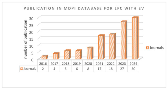
Figure 2. Number of publications in MDPI database for load frequency control and electric vehicles (2016–2024).

In [8], the use of EVs for LFC in restructured power systems has been discussed. This work suggested an enhanced fractional order (FO) controller for robust LFC, taking bilateral transactions into account, and an aggregate model of EV fleets. It selected the best FO controller values in several circumstances using the flower pollination algorithm. The effectiveness of the suggested control approach was confirmed by the simulations that were run. This study offered a chance to develop new grid management goods and services while highlighting the potential of EVs to engage in various ancillary activities in competitive electric markets.

In another study, an adaptive resilient LFC scheme with energy constraints was presented for smart grid subsystems that are subject to denial-of-service (DoS) attacks. This study’s initial section presented a robust triggering communication mechanism in which the uncertainty item brought on by DoS attacks was one of the triggering conditions. In order to lessen the load on communication and thwart denial-of-service attacks, the second section presented an adaptive resilient event-triggering LFC scheme in which the event-triggering parameter can be dynamically changed. Finally, using Lyapunov theory, a stability condition for proportional integral-based LFC systems was determined. Furthermore, case studies based on the various LFC power generation systems—including the one-, two-, and three-area models—were conducted. By comparing the proposed adaptive resilient LFC scheme with resilient event-triggering LFC systems and event-triggering LFC schemes in terms of defense effect and average triggering duration, the simulation results clearly revealed that the suggested adaptive resilient LFC scheme could lower the communication cost while resisting DoS attacks [9].

In smart grids (SGs), the work in [10] examined an event-triggered mechanism (ETM) for multiple frequency services of electric vehicles (EVs). A novel SG model featuring multiple EV agents and an ETM was unveiled. To lessen the strain on network capacity, ETM was implemented. EVs were used to reduce frequency oscillations in the system in both primary and secondary frequency services. The integration of SOC control, an ETM variable resulting from ETM control, and a time-varying delay in the state and control input vectors led to the derivation of a mathematical model for the system. Comprehensive SG simulations with three EV agents were conducted to verify the suggested management plan [10].

In [11], a hybrid power system was successfully planned as an isolated MG with the use of Vehicle-to-Grid (V2G) and the Tidal Power Unit (TPU). The main LFC controller proposed was a new fractional gradient descent (FGD) based on a single-input interval type-2 fuzzy logic controller (SIT2-FLC), where the LFC performance was improved by carefully adjusting the SIT2-FLC’s footprint of uncertainty (FOU) coefficient. To create the additional control action, a deep deterministic policy gradient (DDPG) with the actor-critic framework was also taken into consideration. Finally, a model-in-the-loop (MiL) simulation was run to evaluate the systemic applicability and viability of the recommended design approach.

An overview of the most recent studies on EV charging stations was provided in another study, which also emphasized some significant problems and difficulties with power architecture design, energy storage methods, microgrid control systems, and energy management optimization. Furthermore, the hierarchical control system, which provides decoupled control objectives in various tiers of microgrid systems for EV charging, is explicitly described. In-depth research was performed on common coordinated control methods and energy management plans intended to maximize the efficiency of EV charging stations [12,13].

By providing high virtual inertia and online controlling the charging level, the suggested controller can help inductive electric vehicle (EV) charging systems respond to grid frequency variations in an efficient manner. Utilizing streamlined digital circuits in [14], a novel IPT multi-power level controller was developed. The suggested multi-power level controller included the virtual inertia control/controller (VIC), which measures the grid frequency and modifies the IPT’s charge level online. As a result, the power transfer from the grid to the EV can be controlled in response to changes in grid frequency by using the suggested VIC IPT charger to manage the switching cycles. Simulated data were given to demonstrate how well the suggested VIC IPT power controller responds to variations in the power grid [14].

Within the industry, traditional single-loop controllers might not provide stable performance in the event of altered operating conditions [15]. As an alternative, two-loop cascade fuzzy structured controllers are most effective in nonlinear systems and can demonstrate notably strong performance in dynamic environments. Therefore, taking into account different physical constraints from a practical standpoint, a unique optimal cascade fuzzy-fractional order integral derivative with filter (CF-FOIDF) controller was used for 2-area thermal and hydrothermal PSs. Because of the physical limitations that require an energy storage system, electric vehicle (EV) batteries were used in this study to help power plants quickly arrest oscillations in the system frequency after load demands. The control areas of PSs included a consolidated model of EV fleets. The suggested approach proved to be reliable and effective in providing end customers with consistent, high-quality electrical power [15].

A sigma-modified adaptive control technique was introduced in a different work to improve the charging profile in an EV charging station with several objectives. For bi-directional EV charging, this algorithm additionally guaranteed a continuous charging profile with controller stability and durability. In order to provide better power quality operation even in the presence of grid distortions, the sigma-mod adaptive controller offered an iterative error convergence at each clock interval of supply voltage dynamics. Through maximum power point operation, a solar photovoltaic (PV) array and battery energy storage work together to support ancillary services and further improve the reliability of EV charging chances. For bi-directional EV charging, multivariable sliding mode control and rule-based phase-shift adaptation at various power transformation stages ensure faster convergence, reduced parameters uncertainty, and controller stability [16].

A controller known as a Static Synchronous Series Compensator (SSSC) was used to lessen disruptions in networks of interconnected systems. It is a device known as the Flexible AC Transmission System (FACTS), which efficiently lowers transmission line variations to guarantee a steady-state frequency. The objective of this work [17] was to optimize SSSC parameters within the MATLAB environment by applying the RAT optimization technique, with the goal of reducing frequency variations caused by unknown loads from EV charging stations.

An ideal dispatching control for the EV aggregator was created in a different study. The EV aggregator can give the system regulation capacity with the suggested control scheme while guaranteeing that each individual EV would have adequate SOC. By operating at a faster time- step, the suggested control made it possible for EV aggregators to make better use of EVs. MATLAB and Simulink simulations were run to assess the effectiveness and performance of the suggested dispatching controller [18].

In [19], in order to regulate the system frequency in a networked microgrid system, a secondary controller was created and put into use. Energy-storing units (ESUs), synchronous generators, and renewable energy resources (RESs) made up the suggested power system. Photovoltaic (PV) and wind turbine generator (WTG) units were examples of RESs. A battery and a flywheel made up the ESU. The implemented MA-PID controller delivers and is capable of controlling system frequency under a variety of load demand variations and renewable energy sources, according to the results of the validation comparisons.

In [20], the paper presents an extensive literature review and a critical evaluation of the current state of optimal multi-objective planning for DG installation in the power network, considering various objective functions and their associated constraints. This article examines the implementation of optimization methods for distributed generation planning in radial distribution networks from various power system performance perspectives; it explores the application of various types of DG, distribution models, DG parameters, and mathematical approaches; and it looks at the involvement of different countries in the specified DG positioning and sizing challenge.

From the literature review, the field is still open for study and improvement for electrical vehicle fast charging station location as a dynamic load for frequency control using more accurate optimization methods such as Particle Swarm. Additionally, the use of EVFCSs can produce additional flexibility and stability to the grid by compensation in supply–demand balancing during transit disturbances. The focus of this paper is to investigate the effectiveness of using EVFCSs as a dynamic load for LFC in power systems. This study comprised the optimal location of EVFCSs as a first stage. The output of the first stage will be included in the optimal controller selection to make it the best DR for different network disturbances as the second stage. The Particle Swarm Optimization (PSO) model is utilized to select the best siting of EVFCSs using transient voltage drop and frequency nadir parameters. Optimal control of the dynamic EVFCS load is considered as a second stage in this study using the PSO method as well for the PID controller. The parameters of the PID controller are obtained to effectively aid power system stability during disturbances. The proposed model is applied to the Kundur Power System and IEEE 39 bus system for three types of system disturbances: generation reduction, load reduction, and line faults.

3. Optimal Siting of EVFCS Model Using Particle Swarm Optimization Model

The complex nonlinear optimization problem has a known solution. They came up with the idea of using a particle swarm to optimize functions [21]. We assume an n-dimensional function’s global maximum, which is defined as Equations (1) and (2) (see Figure 3):

$$x_1^2+x_2^2=f_1$$

(1)

$$1+x_1\mathit{sin}4\pi x_2-x_2\mathit{sin}\left(4\pi x_1+\pi \right)=f_2$$

(2)

where $x_1$ and $x_2$ represent the given function variables set.

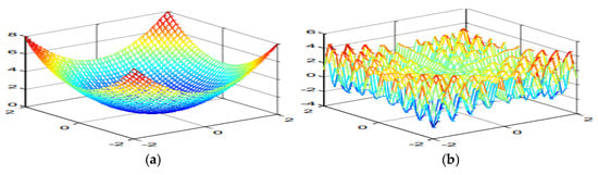
Figure 3. Functions $f_1$ and $f_2$ plots.

A swarm of particles is maintained via the Particle Swarm Optimization (PSO) algorithm, a multi-agent parallel search method. Each particle in the swarm represents a potential solution. Every particle travels through a multidimensional search space, modifying its position based on its own experiences as well as those of its neighbors. Assuming that $x_i^t$ represents the position vector of particle (i) in the multidimensional search space at a given time step (t), each particle’s position in the search space is updated by the following equation:

$$x_i^{t+1}=v_i^{t+1}+x_i^t with x_i^0~ U(X_{min},X_{max})$$

(3)

where $v_i^{t+1}$ is the particle’s velocity vector, which propels the optimization process and represents each particle’s collective experience knowledge as well as its own experience knowledge, and $U\left(X_{min},X_{max}\right)$ is the uniform distribution with respect to its minimum and maximum values.

As a result, in a PSO approach, every particle is started at random and assessed to determine fitness as well as the global best (the best value of every particle in the swarm) and personal best (the best value of every particle). Following that, a loop begins to identify the best answer. The loop updates each particle’s position based on its current velocity after updating each particle’s velocity first using the personal and global bests [22].

In our proposed siting model, the transient stability parameters in terms of voltage drop and rate of change of frequency (ROCOF) are considered. We modeled the problem as optimal power flow with objective function minimizing the voltage drop ($\Delta \mathit{V}$) and the rate of change of frequency (ROCOF) after a disturbance:

$$Min \left(\Delta V\right)= {\sum }_{i=1}^N\left|V_i^{+}-V_i^0\right|$$

(4)

where V_i⁺ and $V_i^0$ are the voltage at bus (i) after a system disturbance and before a disturbance resulting from power flow analysis, respectively.

$$Min \left(ROCOF\right)={\sum }_{i=1}^N{\displaystyle \frac{{\Delta P}_i^{imbalance}-{(X}_i\times P_{EV})}{P_{Load}}} \times {\displaystyle \frac{f_0}{2H}}$$

(5)

where f₀ is the nominal frequency and H is the equivalent system inertia that can be calculated using Equations (6) and (7):

$$H= {\displaystyle \frac{\frac{1}{2}J {\omega }^2}{S}}$$

(6)

$$H_{sync}= {\displaystyle \frac{\sum _{i=1}^N{H}_i {SG}_i}{\sum _{i=1}^N{SG}_i}}$$

(7)

where J is the total momentum of inertia of the system in (kgm²) and S is the rated power in (MVA) of the system synchronous generators.

In order to have one multi-objective function for optimal power flow, Equations (4) and (5) have been normalized through being divided by the maximum voltage drop in Equation (4), and the maximum rate of change of frequency can be acceptable in Equation (5). In our proposed work, both voltage drop and ROCOF have the same weights; however, this can be updated by using different weights of w₁, w₂; Equation (8).

$$Min \left(OF\right)=w_1 {\displaystyle \frac{\sum _{i=1}^N\left|V_i^{+}-V_i^0\right|}{{\Delta V}^{max}}}+w_2{\displaystyle \frac{\sum _{i=1}^N\frac{{\Delta P}_i^{imbalance}-{(X}_i\times P_{EV})}{P_{Load}} \times \frac{f_0}{2H}}{{ROCOF}^{max}}}$$

(8)

The generation–load balance constraint will be used to choose the impact of adding EVFCS in that bus after disturbance, as follows:

$${\sum }_{i=1}^N\left|{PG}_i^{+}-{PLoad}_i^{+}\right|\ge {(X}_i\times P_{EV})$$

(9)

where PG_i⁺ and PLoad_i⁺ are the generator output power and the load power required at bus (i) after a system disturbance, respectively. X_i is a flag variable taking “1” if EVFCS is installed at bus (i) and “0” otherwise. P_EV is EVFCS power rating in KW.

For selecting only one place for installing EVFCS, the following constraint has to be added:

$${\sum }_{i=1}^N{X}_i\le 1$$

(10)

The bus that has the value X_i equal to “1” is the best location for installing EVFCS with a minimum value of ΔV and ROCOF.

Accordingly, the optimal PID controller design using Particle Swarm Optimization model is described in the following section.

4. Optimal Design for PID Controller for EVFCS Using PSO Method

4.1. PID Control

Because PID control works so well, it is a widely used control approach in many different applications. Three fundamental concepts are used in this control technique, which is called proportional–integral–derivative (PID) control. It functions as a feedback control system. The PID controller determines the proper input signal to produce the desired system behavior by taking these terms into account. To achieve optimal performance, the parameters (P, I, and D) are adjusted according to the unique features of each control system [23]. The output of a PID controller is calculated as follows according to Equation (11) [24]:

$$u(t)=Kp\times e(t)+Ki\times \int e(t)dt+Kd\times de(t)/dt$$

(11)

where u(t) is the output signal of the controller, e(t) is the error signal, and Kp, Ki, and Kd are the proportional, integral, and derivative gains, respectively. ∫e(t)dt is the integral of the error over time. de(t)/dt is the derivative of the error with respect to time. The discrete form of the PID controller equation can be determined as Equation (12) [23]:

$$u\left(k\right)=Kp\times e\left(k\right)+Ki\times \Sigma e\left(n\right)+Kd\times \left(e\right(k)-e(k-1\left)\right)$$

(12)

where u(k) is the control signal at time k, e(k) is the error at time k, and Σe(n) represents the sum of errors from n = 0 to k − 1.

A PID controller’s parameters must be tuned in order to produce the desired performance. There are several approaches available for this aim, and each has pros and cons of its own. The Ziegler–Nichols approach, the Cohen–Coon method, the trial-and-error method and optimization techniques are some of the commonly employed strategies [22,25]. Several factors, including system complexity, resource availability, and required performance standards, play a role in the tuning method selection process. Although optimization techniques are very accurate, they are also typically more complicated. These methods apply mathematical optimization techniques to determine the optimal values of the PID parameters. In order to obtain better control performance and efficiency, the PID controller used by the EV station is optimized in this research using Particle Swarm Optimization (PSO).

4.2. PID PSO

Inspired by the social behavior of fish or birds in a flock, the optimization approach known as Particle Swarm Optimization (PSO) was created. Each particle in PSO begins at random in multidimensional space and has two properties: position and velocity. A swarm is believed to have a specific size [26,27]. After moving over a predetermined area, each particle keeps track of the optimal location in relation to the value of the goal function. PSO has been extensively employed as a clever technique for PID parameter optimization for LFC applications because of its consistent outcomes when compared to alternative approaches [28,29].

Particle Swarm Optimization (PSO) algorithm procedures are as follows (see Figure 4) [30,31]:

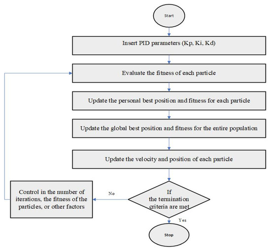
Figure 4. Flowchart of Particle Swarm Optimization (PSO) algorithm.

Initialize a population of particles, where each particle represents a set of PID parameters (K_p, K_i, K_d).

Evaluate the fitness of each particle by applying the objective function to its current position. The objective function is maximizing the damping ratio of the dominant mode in the system.

Update the personal best position and fitness for each particle based on its own best performance.

Update the global best position and fitness for the entire population. The global best position is the best position that any particle has found so far.

Update the velocity and position of each particle. The velocity of a particle is a measure of how much the particle moves in the next iteration. The position of a particle is updated by adding its velocity to its current position. The velocity and position of each particle are updated using Equations (13) and (14) [32]:

$${ v}_i\left(t+1\right)=w\times v_i\left(t\right)+c1 \ast rand\left(\right)\times \left(pbes{t}_i-x_i\left(t\right)\right)+c2 \ast rand\left(\right)\times (gbest-x_i(t\left)\right)$$

(13)

$$x_i(t+1)=x_i\left(t\right)+v_i(t+1)$$

(14)

where w is the inertia weight, which controls how much the particle’s velocity is influenced by its previous velocity; c1 and c2 are acceleration coefficients, which control how much the particle’s velocity is influenced by its personal best position and the global best position, respectively, where rand () generates a random number between 0 and 1.

1.

Check if the termination criteria are met. The termination criteria are a set of conditions that indicate when the algorithm should stop. The termination criteria can be based on the number of iterations, the fitness of the particles, or other factors.

2.

If the termination criteria are not met, go back to step 2. The algorithm repeats steps 2–6 until the termination criteria are met.

4.3. EV Station Modeling in PSS/E

It should be noted that the Second-Generation Generic Model (SGGM) is primarily applicable to steady-state positive sequence analysis [33] and has been officially approved for utilization in WECC studies. To provide a visual representation, Figure 5 depicts the schematic structure of the SGGM [34]. The PSSE software has a Second-Generation Generic Model (SGGM) that comprises three primary modules: the renewable energy generator/convertor module version A (REGC_A), the renewable energy electrical control module version C (REEC_C), and the renewable energy plant control module version A (REPC_A) [8]. These three modules are employed to model the dynamic characteristics of EV fast charging stations since they are typically used to emulate the energy storage system dynamic behavior in PSSE; the only difference is to modify the power flow data in the EV station as a negative generation. Hence, the dynamic modeling of the EV fast charging station is based on the dynamic modeling of the energy storage system used in PSSE.

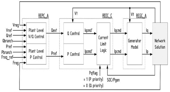
Figure 5. The schematic structure of the SGGM.

5. Experimental Setup and Results

The experimental setup starts with running the well-known OPF with minimum fuel cost. The output of OPF will be input for PSSE simulation that is used to study different disturbances: generation reduction, load reduction, and line faults. ΔV^max and ROCOF^max are the two outputs of PSSE. After that, we applied our proposed method (Stage 1) to select the optimal location of EVFCS. In this step, the OPF objective function is changed to be similar to Equation (8) with the consideration of w₁ equals w₂. The OPF will call PSSE in each iteration to measure the current transient voltage drop ΔV and the current transient rate of change of frequency ROCOF during disturbances if EVFCS is installed in the bus (i). The proposed PSO is applied with the proposed dynamic modeling of EVFCS using PSSE to select the best EVFCS location as a result of Stage 1. After this stage, the location of EVFCS is kept fixed, and the second stage is applied. The second stage uses PSO to select the best PID parameters that reduce transient voltage drop ΔV and transient rate of change of frequency ROCOF, similar to the procedures in Figure 4. Finally, the results of Stage 2 reveal the best K_P, K_I, and K_D parameters for the PID controller installed in EVFCS at the best location obtained from Stage 1.

5.1. Simulated Network

Figure 6 and Figure 7 show Kundur’s model and the IEEE 39 bus system. In Kundur’s model under typical working conditions, electricity flows from area 1 to area 2, and the network has four machines (G1 and G2 belong to area 1, G3 and G4 belong to area 2), with an overall generation capacity of 2819 MW. The network is designed with several buses and transmission lines connecting the loads to generators. The two areas are interconnected through a series of transmission lines with specific distances between buses: 25 km between Bus 1 and Bus 5, 10 km between Bus 5 and Bus 6, 110 km between Bus 6 and Bus 7, another 110 km between Bus 7 and Bus 8, and a further 110 km between Bus 8 and Bus 9. From Bus 9 to Bus 10, the distance is 10 km, followed by 25 km from Bus 10 to Bus 11 (Figure 6).

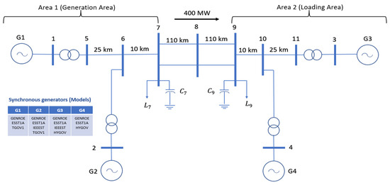
Figure 6. Kundur system model in PSSE.

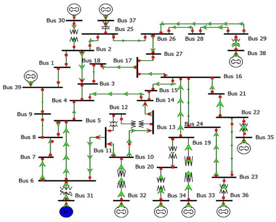
Figure 7. IEEE 39 model in PSSE.

In addition, the network includes reactive power elements at load area buses to manage voltage levels and stability. Capacitor C7 with a capacity of 200 MVAr and Load L7 with a capacity of 967 MW are present at Bus 7, while Capacitor C9 with a capacity of 350 MVAr and Load L9 with a capacity of 1767 MW are at Bus 9. The total active power of Kundur’s system is 2734 M. There is a power flow of 400 MW from area 1 to area 2, indicating the amount of transfer of power through the interconnection. This model is typically used to analyze the power flow, stability, and reliability of the interconnected power system.

In order to apply the proposed location model to a larger transmission network, the IEEE 39 test system was selected. It has 10 generator machines, 46 branches, and 19 loads. The overall generation capacity of the system is 6298 MW, where the total load connected is 6097 MW (Figure 7).

5.2. Case Studies

To evaluate the performance of the methodology proposed in this study, simulations were conducted using the PSSE software (version 36) for Kundur’s system as a case study, as seen in Figure 6. The PSSE model used in the simulations was obtained from the Illinois Center for a Smarter Electric Grid (ICSEG) at the University of Illinois at Urbana-Champaign; PSSE models. To analyze the simulation results and assess the effectiveness of using PID control with EV stations, and examine the simulation findings, an assessment was carried out with a focus on four specific buses in Kundur’s system. These buses (1, 3, 7, and 9) were chosen based on an observability analysis that means two points should be in the generation area and two points in the loading area. Hence, at least four buses are required to observe the dynamic response of the system stability in two areas. However, the IEEE 39 bus test system requires only two buses (38 and 39) since the interconnection of the system makes it considered as one area that includes generation and load. Three different disturbances are considered in this study: generation reduction (50 MW, 100 MW), load reduction (50 MW, 100 MW), and a line fault. Since there are lines between Bus 7, Bus 8, and Bus 9 connecting the two areas in Kundur’s system, the system response during a bus fault at Bus 8 was analyzed. However, the heavy line that connects Bus 19 and Bus 16 was selected for line fault in the IEEE 39 bus test system. Table 1 shows the power flow analysis of IEEE 39 before installing the EV charging stations.

Table 1. IEEE 39 power flow analysis without EV charging stations’ installation using PSSE software.

Bus Number	P-Load (MW)	Q-Load (MVAr)	P-Generation (MW)	Q-Generation (MVAr)
3	322	2.4	-	-
4	400	184	-	-
7	233.8	84	-	-
8	522	176	-	-
12	7.5	88	-	-
15	320	153	-	-
16	329.4	32.3	-	-
18	158	30	-	-
20	628	103	-	-
21	274	115	-	-
23	274.5	84.6	-	-
24	308.6	−92.2	-	-
25	224	47.2	-	-
26	139	17	-	-
27	281	75.5	-	-
28	206	27.6	-	-
29	283.5	26.9	-	-
30	-	-	250	132.94
31	9.2	4.6	547.33	−45.97
32	-	-	650	185.27
33	-	-	632	101.14
34	-	-	508	161.38
35	-	-	650	200.25
36	-	-	560	97.19
37	-	-	540	−7.79
38	-	-	830	18.12
39	1104	250	1000	73.60

The EV station size is chosen to be equal to 1% of the system generation that is around 30 MW and 65 MW in Kundur’s system and the IEEE 39 bus test system, respectively.

5.3. PSO Location Results of Optimal EV Station Location

The PSO location model was applied to Kundur’s system to evaluate the optimal locations of EVFCSs that minimize both transient voltage drop and frequency nadir parameters during generation reduction, load reduction and line fault disturbances. The PSO location model ranks the system buses from 1 to 11, where 1 is the best location and 11 is the worst location for EVFCS as DR for LFC. Table 2 shows the result of the PSO location model for Kundur’s system where Bus 1 then Bus 4 were the optimal locations with weights of 0.3332 and 0.4296, respectively. Bus 1 is the optimal location in the generation area, and Bus 4 is the optimal location in the load area. The worst places for installing EVFCS from the LFC point of view are Bus 8, Bus 7, and Bus 6 since these buses connect the generation area with the tie line.

Table 2. The best locations for dynamic EVFCSs in Kundur’s system.

	BUS-1	BUS-2	BUS-3	BUS-4	BUS-5	BUS-6	BUS-7	BUS-8	BUS-9	BUS-10	BUS-11
PSO Rank	#1	#7	#8	#2	#4	#9	#10	#11	#6	#3	#5
PSO weight	0.3332	0.8227	0.9330	0.4296	0.5440	1.1287	1.2999	2.0115	0.7020	0.4637	0.6592

For the IEEE 39 bus test system, the PSO location model was applied, and the result of optimal EVFCS locations as DR for LFC is shown in Table 3.

Table 3. The best locations for dynamic EVFCS in IEEE 39 bus system.

The Best Location	PSO Rank	PSO Weight
Bus 39	#1	0.008307
Bus 1	#2	0.020505
Bus 9	#3	0.020624
Bus 30	#4	0.027486
Bus 37	#5	0.035829

Bus 39 then Bus 1 were the optimal locations for EVFCSs as DR for LFC with PSO weights of 0.008307 and 0.020505, respectively. Since more power was flowing to buses near Bus 39 and Bus 1, these buses are more suitable for LFC, as the PSO location model showed in its result.

To validate the result of the best spot to install EVFCSs as DR for LFC, a sensitivity analysis is carried out. In this analysis, every potential location in Kundur’s system for the EV station is evaluated, and the optimum options are shown. The EV station is first located on a particular bus as part of the investigation procedure. The system, which is referred to as a Single-Input Single-Output (SISO) system, is then represented by a transfer function that is created. The ideal observation position provides the system’s output, and the active power reference of the EV station serves as its input. Equation (15) describes the power system’s identification with respect to the placement bus signals [35]:

$$G\left(s\right)={\displaystyle \frac{R_1}{s-{\lambda }_1}}+{\displaystyle \frac{R_2}{s-{\lambda }_2}}+\dots +{\displaystyle \frac{R_m}{s-{\lambda }_m}}$$

(15)

The eigenvalues of the system are denoted by ${\lambda }_i$, while the system residue, represented by $R_i$, is a measure of the interaction between mode observability and controllability. When ${\lambda }_i$ is unobservable or uncontrollable,${ R}_i=0$. In complex power systems, various equipment is typically associated with one or more modes within the system. Among these modes, inter-area oscillation modes are particularly noteworthy. They can be effectively observed through the controlled system $G\left(s\right)$ when there is a stronger level of mode observability and controllability compared to other modes [36]. These inter-area oscillation modes carry significant importance in the overall dynamics and stability analysis of complex power systems. The residues provide valuable insights into the effectiveness of control strategies and the ability to observe oscillation modes within the power system. By evaluating the residues, researchers can assess and validate the controllability and observability characteristics of different modes, allowing for the identification of critical modes that require attention and damping measures [37,38]. Table 4 presents the residue analysis of when the EV station is placed at each bus for Kundur’s system. It can be concluded that generation area buses have a higher residue magnitude, which means higher controllability. For example, among the generation area buses, the center of the generation (Bus 1) is the best placement of the EV, and the loading center of generation area (Bus 7) is the worst placement.

Table 4. EV bus placement sensitivity analysis based on residue magnitude.

EV Bus	Residue Analysis Data
	Res. Angle	Res. Mag	Os. Freq	Dam. Ratio
Bus 1	−105.8447	0.000983153	0.639647	8.5331082
Bus 2	−127.9539	0.000621572	0.649031	7.3502683
Bus 3	−123.9805	0.000512024	0.627557	7.1490643
Bus 4	−118.1057	0.000483824	0.622625	8.2147794
Bus 5	−121.2728	0.000848788	0.633606	8.3939793
Bus 6	−131.7225	0.000759179	0.647551	9.9286084
Bus 7	−142.8167	0.000542452	0.650582	10.175342
Bus 8	NA	NA	NA	NA
Bus 9	−119.29254	0.00057633	0.596478	11.770109
Bus 10	−122.4843	0.000388127	0.610599	7.511333
Bus 11	−125.1513	0.000595481	0.624548	9.1920959

This sensitivity analysis validates the outcomes from the PSO location model from a controllability and observability perspective.

5.4. PSO—PID Model Results

A typical PID controller and a base case scenario with no control input for each EV station placement bus were compared in the first comparison to examine the performance of utilizing a PID controller with the PSO model for EV stations. The frequency difference response comparison for the chosen four buses, Buses 1, 3, 7, and 9, with the EV station installed is shown in Figure 8a–d. The findings unequivocally show that in comparison to the other scenarios, the PID controller with PSO greatly enhances the dominant oscillation mode’s damping.

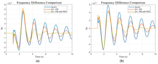
Figure 8. Frequency difference response between generation area and loading area when EV station placed (a) Bus 1, (b) Bus 3, (c) Bus 7, and (d) Bus 9.

Secondly, the performance results of the PID controller with PSO for different EV station placement buses are presented in Figure 9.

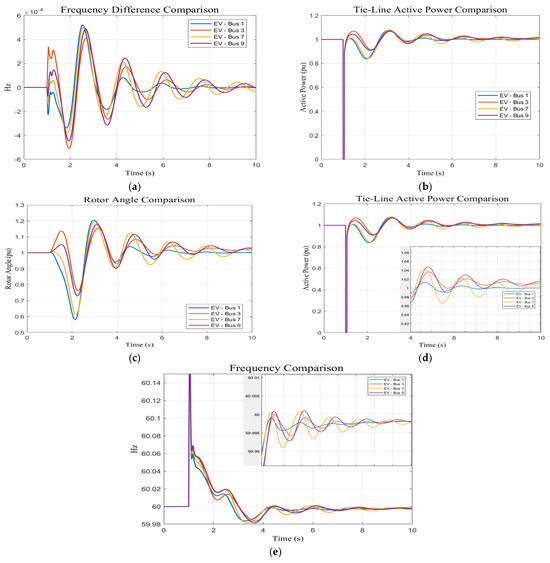
Figure 9. (a) Frequency difference response, (b) tie line active power response, (c) rotor angle response comparison, (d) tie line active power response, and (e) frequency response comparison when PID (PSO) is attached with the selected buses.

Figure 9 shows the frequency response, frequency difference, active power tie line, and rotor angle for each case. The analysis shows that by placing the EV station at Bus 1, the generation center of the generation area, it has the highest impact on enhancing system stability. On the other hand, Bus 7, the loading center of the generation area, has a relatively smaller impact. Lastly, Bus 9, the loading center of the loading area, has the least influence on system stability. In order to assess the power of optimizing PID parameters using the PSO-PID model, a comparison between the best bus placement with traditional PID and the worst bus placement with PID-PSO is presented in Figure 10 and Figure 11. It shows that Bus 1 of Kundur’s system and Bus 39 then Bus 1 in the IEEE 39 bus system are the best locations for dynamic EVFCSs (Table 2 and Table 3).

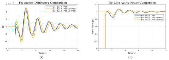
Figure 10. (a) Frequency difference response and (b) tie line active power response comparison between Bus 1 with traditional PID and Buses 7 and 9 with PID-PSO for Kundur’s system.

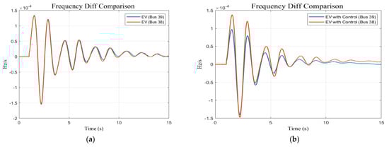
Figure 11. Frequency difference response between Bus 39 and Bus 38 (a) without control and (b) with control PID-PSO for the IEEE 39 test system.

6. Discussion

According to this study, the best way to improve the system stability of Kundur’s system is to locate the EV station at Bus 1, which is the generation center of the generation area. After that, Bus 4, the loading area’s generation center, shows a favorable influence, but Bus 7, the generation area’s loading center, has comparatively less impact. Finally, the loading center of the loading area, Bus 9, has the least impact on the stability of the system. The results demonstrated that the PID controller with PSO significantly increases the dominant oscillation mode’s damping when compared to the other cases. Generally, Bus 1 then Bus 4 of Kundur’s system and Bus 39 then Bus 1 in the IEEE 39 bus system are the best locations for dynamic EVFCSs. If the EVFCS is located in least bus controllability and observability, the PID parameters have to be optimized in order to enhance their capability using the PSO-PID model.

To validate our main findings of the proposed work, we compare the stability performance of the results of Kundur’s system with the methods in [39]. Three controlling methods were highlighted in [39]: nonlinear disturbance observer (NDO), nonlinear disturbance observer based on adaptive super twisting sliding mode control (ST-SMC), and PI-PSO with conventional control as well as our proposed PID-PSO. The comparison between these methods based on frequency deviation (Δf) is shown in Table 5.

Table 5. Comparison between different LFC techniques in Kundur’s system four machines.

LFC Method	f1 (±Hz)Δ	f2 (±Hz)Δ
EV-PID Control	0.4153	0.4072
NDO [39]	0.375	0.375
ST-SMC [39]	0.35	0.35
PI-PSO [39]	0.552	0.546
Proposed EV PID-PSO	0.2453	0.22303

It is clear from the above comparison that adding an EV charging station as a dynamic load for LFC enhances stability performance in terms of frequency deviation. EV-PID control overcame the performance of PI-PSO due to the capability of being dynamic when modeling EV station in this proposed work. When using PID-PSO with EV stations as dynamic load, the deferential covers the previous events, the integration covers the future events, and the proportional covers the amplitude needed. Hence, this proposed technique is the most suitable for the purpose of a dynamic load as LFC.

7. Conclusions

This study investigates the viability of employing EVFCSs as a dynamic load for LFC in power systems. The ideal placement of the EVFCS as well as the appropriate controller choice to make it the best DR for various network disruptions were included in this study. Using transient voltage drop and frequency nadir parameters, the Particle Swarm Optimization model is used to determine the optimal location for the EVFCS. The second stage in this study uses the optimal locations from the PSO location model in the PSO-PID controller model. The optimal PID parameters to control the dynamic EVFCS load are evaluated then applied to support efficient power system stability during disturbances. Three types of system disturbances were addressed by the suggested models, namely generation reduction, load reduction, and line faults.

Intelligent control techniques will be one of the main research directions for similar studies focusing on stability performance with the integration of LFC. EV charging stations show positive impacts on system dynamics and improving the controlling techniques to be more rapid, to be focused on in future work. The economic feasibility of using the EVFCS as LFC is another extension of this work to estimate how compensation can be offered to EV users for any possible damage or charging speed reduction. Lastly, this work can be extended by including the dynamic behavior of all loads instead of only EVs. When modeling the dynamic of all loads similar to Ref. [40], the assessment will be more realistic and practical.

References

- Li, Z.; Khajepour, A.; Song, J. A comprehensive review of the key technologies for pure electric vehicles. Energy 2019, 182, 824–839. [Google Scholar] [CrossRef]
- Amjad, M.; Ayaz, A.; Mubashir, H.; Tariq, U. A review of EVs charging: From the perspective of energy optimization, optimization approaches, and charging techniques. Transp. Res. Part D Transp. Environ. 2018, 62, 386–417. [Google Scholar] [CrossRef]
- Adil, M.; Mahmud, M.P.; Kouzani, A.Z.; Khoo, S. Energy trading among electric vehicles based on Stackelberg approaches: A review. Sustain. Cities Soc. 2021, 75, 103199. [Google Scholar] [CrossRef]
- Barman, P.; Dutta, L.; Bordoloi, S.; Kalita, A.; Buragohain, P.; Bharali, S.; Azzopardi, B. Renewable energy integration with electric vehicle technology: A review of the existing smart charging approaches. Renew. Sustain. Energy Rev. 2023, 183, 113518. [Google Scholar] [CrossRef]
- Khan, I.A.; Mokhlis, H.; Mansor, N.N.; Illias, H.A.; Awalin, L.J.; Wang, L. New trends and future directions in load frequency control and flexible power system: A comprehensive review. Alex. Eng. J. 2023, 71, 263–308. [Google Scholar] [CrossRef]
- Yoo, Y.; Al-Shawesh, Y.; Tchagang, A. Coordinated Control Strategy and Validation of Vehicle-to-Grid for Frequency Control. Energies 2021, 14, 2530. [Google Scholar] [CrossRef]
- Deb, N.; Singh, R.; Brooks, R.R.; Bai, K. A Review of Extremely Fast Charging Stations for Electric Vehicles. Energies 2021, 14, 7566. [Google Scholar] [CrossRef]
- Debbarma, S.; Dutta, A. Utilizing Electric Vehicles for LFC in Restructured Power Systems Using Fractional Order Controller. IEEE Trans. Smart Grid 2017, 8, 2554–2564. [Google Scholar] [CrossRef]
- Lu, K.D.; Zeng, G.Q.; Luo, X.; Weng, J.; Zhang, Y.; Li, M. An Adaptive Resilient Load Frequency Controller for Smart Grids with DoS Attacks. IEEE Trans. Veh. Technol. 2020, 69, 4689–4699. [Google Scholar] [CrossRef]
- Pham, T.N.; Oo, A.M.T.; Trinh, H. Event-Triggered Mechanism for Multiple Frequency Services of Electric Vehicles in Smart Grids. IEEE Trans. Power Syst. 2022, 37, 967–981. [Google Scholar] [CrossRef]
- Khooban, M.H.; Gheisarnejad, M. A Novel Deep Reinforcement Learning Controller Based Type-II Fuzzy System: Frequency Regulation in Microgrids. IEEE Trans. Emerg. Top. Comput. Intell. 2021, 5, 689–699. [Google Scholar] [CrossRef]
- Xie, Y.; Liao, P.; Liang, Z.; Zhou, D. State of Change-Related Hybrid Energy Storage System Integration in Fuzzy Sliding Mode Load Frequency Control Power System with Electric Vehicles. Machines 2025, 13, 57. [Google Scholar] [CrossRef]
- Nagendra, K.; Varun, K.; Pal, G.; Santosh, K.; Semwal, S.; Badoni, M.; Kumar, R. A Comprehensive Approach to Load Frequency Control in Hybrid Power Systems Incorporating Renewable and Conventional Sources with Electric Vehicles and Superconducting Magnetic Energy Storage. Energie 2024, 17, 5939. [Google Scholar] [CrossRef]
- Jafari, H.; Moghaddami, M.; Olowu, T.O.; Sarwat, A.I.; Mahmoudi, M. Virtual Inertia-Based Multipower Level Controller for Inductive Electric Vehicle Charging Systems. IEEE J. Emerg. Sel. Top. Power Electron. 2021, 9, 7369–7382. [Google Scholar] [CrossRef]
- Arya, Y. Effect of electric vehicles on load frequency control in interconnected thermal and hydrothermal power systems utilising CF-FOIDF controller. IET Gener. Transm. Distrib. 2020, 14, 2666–2675. [Google Scholar] [CrossRef]
- Mishra, D.; Singh, B.; Panigrahi, B.K. Sigma-Modified Power Control and Parametric Adaptation in a Grid-Integrated PV for EV Charging Architecture. IEEE Trans. Energy Convers. 2022, 37, 1965–1976. [Google Scholar] [CrossRef]
- Srinivas, C.; Shanmugapriya, S.; Babu, K.R.; Chaturvedula, U.K.; Santoshi, K.P. Control Strategy for Load Frequency Control in Power Systems with Electric Vehicle Charging Stations. In Proceedings of the 2023 3rd Asian Conference on Innovation in Technology, Pune, India, 25–27 August 2023; pp. 1–6. [Google Scholar]
- Cai, S.; Matsuhashi, R. Optimal dispatching control of EV aggregators for load frequency control with high efficiency of EV utilization. Appl. Energy 2022, 319, 119233. [Google Scholar] [CrossRef]
- Boopathi, D.; Jagatheesan, K.; Anand, B.; Samanta, S.; Dey, N. Frequency Regulation of Interlinked Microgrid System Using Mayfly Algorithm-Based PID Controller. Sustainability 2023, 15, 8829. [Google Scholar] [CrossRef]
- Kumar, M.; Soomro, A.M.; Uddin, W.; Kumar, L. Optimal Multi-Objective Placement and Sizing of Distributed Generation in Distribution System: A Comprehensive Review. Energies 2022, 15, 7850. [Google Scholar] [CrossRef]
- Gad, A.G. Particle Swarm Optimization Algorithm and Its Applications: A Systematic Review. Arch. Comput. Methods Eng. 2022, 29, 2531–2561. [Google Scholar] [CrossRef]
- Joseph, S.B.; Dada, E.G.; Abidemi, A.; Oyewola, D.O.; Khammas, B.M. Metaheuristic algorithms for PID controller parameters tuning: Review, approaches and open problems. Heliyon 2022, 8, e09399. [Google Scholar] [CrossRef] [PubMed]
- Borase, R.P.; Maghade, D.K.; Sondkar, S.Y.; Pawar, S.N. A review of PID control, tuning methods and applications. Int. J. Dyn. Control 2021, 9, 818–827. [Google Scholar] [CrossRef]
- Jin, X.; Chen, K.; Zhao, Y.; Ji, J.; Jing, P. Simulation of hydraulic transplanting robot control system based on fuzzy PID controller. Measurement 2020, 164, 108023. [Google Scholar] [CrossRef]
- Dogru, O. Reinforcement learning approach to autonomous PID tuning. Comput. Chem. Eng. 2022, 161, 107760. [Google Scholar] [CrossRef]
- Sengupta, S.; Basak, S.; Peters, R.A. Particle Swarm Optimization: A Survey of Historical and Recent Developments with Hybridization Perspectives. Mach. Learn. Knowl. Extr. 2019, 1, 157–191. [Google Scholar] [CrossRef]
- Freitas, D.; Lopes, L.G.; Morgado-Dias, F. Particle Swarm Optimisation: A Historical Review Up to the Current Developments. Entropy 2020, 22, 362. [Google Scholar] [CrossRef]
- Patel, N.C.; Debnath, M.K.; Sahu, B.K.; Dash, S.S.; Bayindir, R. Application of invasive weed optimization algorithm to optimally design multi-staged PID controller for LFC analysis. Changes 2019, 9, 470–479. [Google Scholar]
- Zeng, N.; Wang, Z.; Liu, W.; Zhang, H.; Hone, K.; Liu, X. A dynamic neighborhood-based switching particle swarm optimization algorithm. IEEE Trans. Cybern. 2020, 52, 9290–9301. [Google Scholar] [CrossRef]
- Guo, X.; Ji, M.; Zhao, Z.; Wen, D.; Zhang, W. Global path planning and multi-objective path control for unmanned surface vehicle based on modified particle swarm opti-mization (PSO) algorithm. Ocean Eng. 2020, 216, 107693. [Google Scholar] [CrossRef]
- Kohler, M.; Vellasco, M.M.; Tanscheit, R. PSO: A new particle swarm optimization algorithm for constrained problems. Appl. Soft Comput. 2019, 85, 105865. [Google Scholar] [CrossRef]
- Sousa-Ferreira, I.; Sousa, D. A review of velocity-type PSO variants. J. Algorithms Comput. Technol. 2017, 11, 23–30. [Google Scholar] [CrossRef]
- Wang, W.; Wang, J. Convex combination of two geometric-algebra least mean square algorithms and its performance analysis. Signal Process. 2022, 192, 108333. [Google Scholar] [CrossRef]
- Wan, Z.; Yu, B.; Li, T.Y.; Tang, J.; Zhu, Y.; Wang, Y.; Raychowdhury, A.; Liu, S. A survey of fpga-based robotic computing. IEEE Circuits Syst. Mag. 2021, 21, 48–74. [Google Scholar] [CrossRef]
- Wang, X.; He, Z.; Yang, J. Electric Vehicle Fast-Charging Station Unified Modeling and Stability Analysis in the dq Frame. Energies 2018, 11, 1195. [Google Scholar] [CrossRef]
- Camacho-Villalón, C.L.; Dorigo, M.; Stützle, T. PSO-X: A component-based framework for the automatic design of particle swarm optimization algorithms. IEEE Trans. Evol. Comput. 2021, 26, 402–416. [Google Scholar] [CrossRef]
- Fakhouri, H.N.; Hudaib, A.; Sleit, A. Multivector particle swarm optimization algorithm. Soft Comput. 2020, 24, 11695–11713. [Google Scholar] [CrossRef]
- Pozna, C.; Precup, R.E.; Horváth, E.; Petriu, E.M. Hybrid particle filter–particle swarm optimization algorithm and application to fuzzy controlled servo systems. IEEE Trans. Fuzzy Syst. 2022, 30, 4286–4297. [Google Scholar] [CrossRef]
- Dev, A.; Anand, S.; Sarkar, M.K. Nonlinear disturbance observer based adaptive super twisting sliding mode load frequency control for nonlinear interconnected power network. Asian J. Control 2021, 23, 2484–2494. [Google Scholar] [CrossRef]
- Saxena, N.K.; Kumar, A. Modelling for Composite Load Model Including Participation of Static and Dynamic Load. In Optimization of Power System Problems: Methods, Algorithms and MATLAB Codes; Springer International Publishing: Cham, Switzerland, 2020; pp. 1–48. [Google Scholar]
Disclaimer/Publisher’s Note: The statements, opinions and data contained in all publications are solely those of the individual author(s) and contributor(s) and not of MDPI and/or the editor(s). MDPI and/or the editor(s) disclaim responsibility for any injury to people or property resulting from any ideas, methods, instructions or products referred to in the content. |
© 2025 by the authors. Published by MDPI on behalf of the World Electric Vehicle Association. Licensee MDPI, Basel, Switzerland. This article is an open access article distributed under the terms and conditions of the Creative Commons Attribution (CC BY) license (https://creativecommons.org/licenses/by/4.0/).