Resource Optimization Method Based on Spatio-Temporal Modeling in a Complex Cluster Environment for Electric Vehicle Charging Scenarios

Abstract

In intelligent cluster systems, the spatio-temporal complexity of agent data collection and resource allocation, as well as the problems in collaborative organizations, present substantial challenges to efficient resource distribution. To address this, a novel self-organizing prediction method for spatio-temporal resource allocation is proposed. In the spatio-temporal modeling part, dilated convolution is applied for time modeling. Its dilation rate grows exponentially with the layer depth, allowing it to effectively capture the time trends of graph nodes and handle long time series data. For spatial modeling, an innovative dual-view dynamic graph convolutional network architecture is utilized to accurately explore the static and dynamic correlation information of the spatial layout of charging piles. Meanwhile, a composite self-organizing mechanism integrating a trust model is put forward. The trust model assists agents in choosing partners, and the Q-learning algorithm of the intelligent cluster realizes the independent evaluation of rewards and the optimization of relationship adaptation. In the experimental scenario of electric vehicle charging, considering charging piles as agents, under the home charging mode, the self-organizing charging scheduling can reduce the total load range by up to 90.37%. It effectively shifts the load demand from peak periods to valley periods, minimizes the total peak–valley load difference, and significantly improves the security and reliability of the microgrid, thus providing a practical solution for resource allocation in intelligent clusters.

1. Introduction

An intelligent cluster system refers to an autonomous intelligent agent system composed of a certain number of homogeneous or heterogeneous, single-function or multi-function intelligent agents. Supported by the sympathetic network, it can utilize sympathetic behaviors such as information exchange and feedback, incentive, and response to achieve autonomous decision-making of agent behaviors, behavior coordination among intelligent clusters, adaptation to the dynamic environment, and, finally, generate the emergence of capabilities to jointly complete specific tasks [1]. The most significant characteristics of such systems are emergence and evolvability. They can implement self-organization, self-adaptation, and reconfiguration mechanisms, and can achieve excellent autonomy, reactivity, proactivity, and sociality [2].

Intelligent cluster systems have the following characteristics in terms of individual perception and collaborative organizational architecture. In terms of individual perception, intelligent agents vary in their data collection capabilities, methods, and the scale of individuals they cover, resulting in uneven data quality in swarm intelligence perception. Moreover, there are complex spatio-temporal correlations in the resource allocation patterns of intelligent agents. This paper will propose a spatio-temporal dependence model. This model can dynamically adjust the resource allocation strategies of intelligent agents according to changes in time and space, which can improve the efficiency of resource utilization and reduce resource waste. In terms of collaborative organizational architecture, intelligent agents need to perceive and act in a dynamic environment while achieving a balance of individual interests and maximizing the group interests within the system. The collaborative organizational structure of the intelligent agent cluster is complex and has to face problems such as uncertainty in the game environment and incomplete decision-making information [3]. Therefore, we believe that the self-organization mechanism is a good choice to solve such problems. It coordinates global behaviors through local rules and improves the robustness and adaptability of the system.

In the relevant research work on intelligent cluster modeling, Niu et al. [4] mentioned the Random Configuration Network (RCN), which ensures the universal approximation property by randomly assigning weights and biases. Brust et al. [5] provided solutions for the combination between group behaviors and spatial topology. Wei et al. [6] comprehensively considered the changes in the energy consumption of agents and the geographical locations of nodes, and proposed a charging strategy for wireless sensor networks based on reinforcement learning. Cao et al. [7] used Deep Reinforcement Learning (DRL) modeling to obtain the paths of mobile chargers (MC). Xu et al. [8] optimized the total travel distance of mobile chargers during the monitoring period through heuristic algorithms. Wang et al. [9] proposed a distance- and energy-oriented charging scheduling algorithm to prevent nodes from being depleted. Han et al. [10] designed a mobile charging algorithm to provide energy replenishment for sensor nodes. Soni et al. [11] used reinforcement learning techniques to optimize charging paths in order to reduce charging costs.

In the above traditional intelligent cluster modeling, researchers usually focus on optimization in the spatial dimension and combine algorithms to plan a series of action sequences for intelligent agent objects. However, this modeling method often neglects the dynamic adjustment in the time dimension; that is, it fails to make full use of time data to optimize the allocation and scheduling of resources. Such an optimization strategy in a single dimension may lead to an unbalanced allocation of resources and low efficiency. Therefore, in order to improve the capabilities of intelligent cluster systems in aspects such as data collection and swarm intelligence perception, it is necessary to introduce a more comprehensive multi-dimensional modeling method in the time–space domain to achieve the dynamic optimization and intelligent scheduling of resources.

Spatio-temporal modeling can comprehensively analyze the data characteristics in both the time and space dimensions. Specifically, by capturing the laws of how data quality changes over time and space, spatio-temporal modeling can identify the periodicity of resource demands and the distribution of hotspots, thus making resource allocation strategies more precise and more adaptable [12]. For example, in the time dimension, the model can predict the peaks and troughs of resource demands in different time periods and achieve rational resource scheduling; in the space dimension, the model can reveal the geographical distribution characteristics of resource demands and guide resources to be inclined towards regions with concentrated demands. In addition, spatio-temporal modeling supports dynamic adjustment and can update resource allocation plans in real time as the environment changes, improving the efficiency of resource utilization and the effectiveness of agent task execution [13].

In the field of multi-agent collaboration, coalitions [14], teams [15], collaborative communities [16], etc., obtain the maximization of individual utilities or complete complex tasks by constructing collaborative organizations, seldom considering the issue of agents joining or leaving collaborative organizations at any time. Multi-agent reinforcement learning techniques have demonstrated excellent performance in games. However, in real-world environments, due to the influence of resource usage limitations and environmental uncertainties, it is difficult for agents to effectively coordinate the utilization of resources and maximize the overall benefits by constructing collaborative organizations [17].

However, intelligent clusters can adjust their structures through self-organization mechanisms to cope with changes in the environment and resources as well as the communication of decision-making information. Self-organization means that in the absence of any external control or influence in the system, the cooperative behaviors of individual entities form a certain pattern. The self-organization mechanism of intelligent clusters can handle massive, multi-dimensional, and complex structures in a dynamic environment. It can effectively abstract valuable features and potential laws in complex systems and describe the dynamic evolution process of the system, such as the addition of new nodes, the disappearance of some nodes, and changes in the connection strength between nodes. Each intelligent agent under the self-organization mechanism of intelligent clusters can adjust its own strategies according to the constantly changing situation and the information obtained through communication, such as cooperation among individuals and games with counterparts [18].

Zeng et al. [19] proposed a multi-agent collaboration framework based on the principle of structural information, which utilizes the optimal coding tree to achieve self-organizing collaboration. Liu et al. [20] put forward an agent organization method that enables multiple agents to interact in a task-based dynamic framework to achieve self-organizing collaboration. Hong et al. [21] proposed MetaGPT, which integrates the artificial workflow into the multi-agent collaboration based on LLM, facilitating the self-organizing cooperation of multiple agents. Chen et al. [22] proposed the AgentVerse framework, realizing that in collaboration, the group performance of multiple agents is better than the sum of the individual performances. Chen et al. [23] proposed a method that can adaptively generate and coordinate multiple differentiated agents to construct agent teams according to different tasks. However, although these studies have achieved remarkable progress in the field of multi-agent collaboration, they still have certain limitations in the trust model among agents and the selection of dynamic partners. To solve this problem, we propose an innovative method, that is, using a composite self-organizing Q-learning algorithm based on a trust model. This method enables agents to utilize their own experiences and the opinions of other agents when selecting partners, thereby improving the communication and coordination capabilities of the system and its adaptability to the dynamic environment, and achieving the rational allocation of resources.

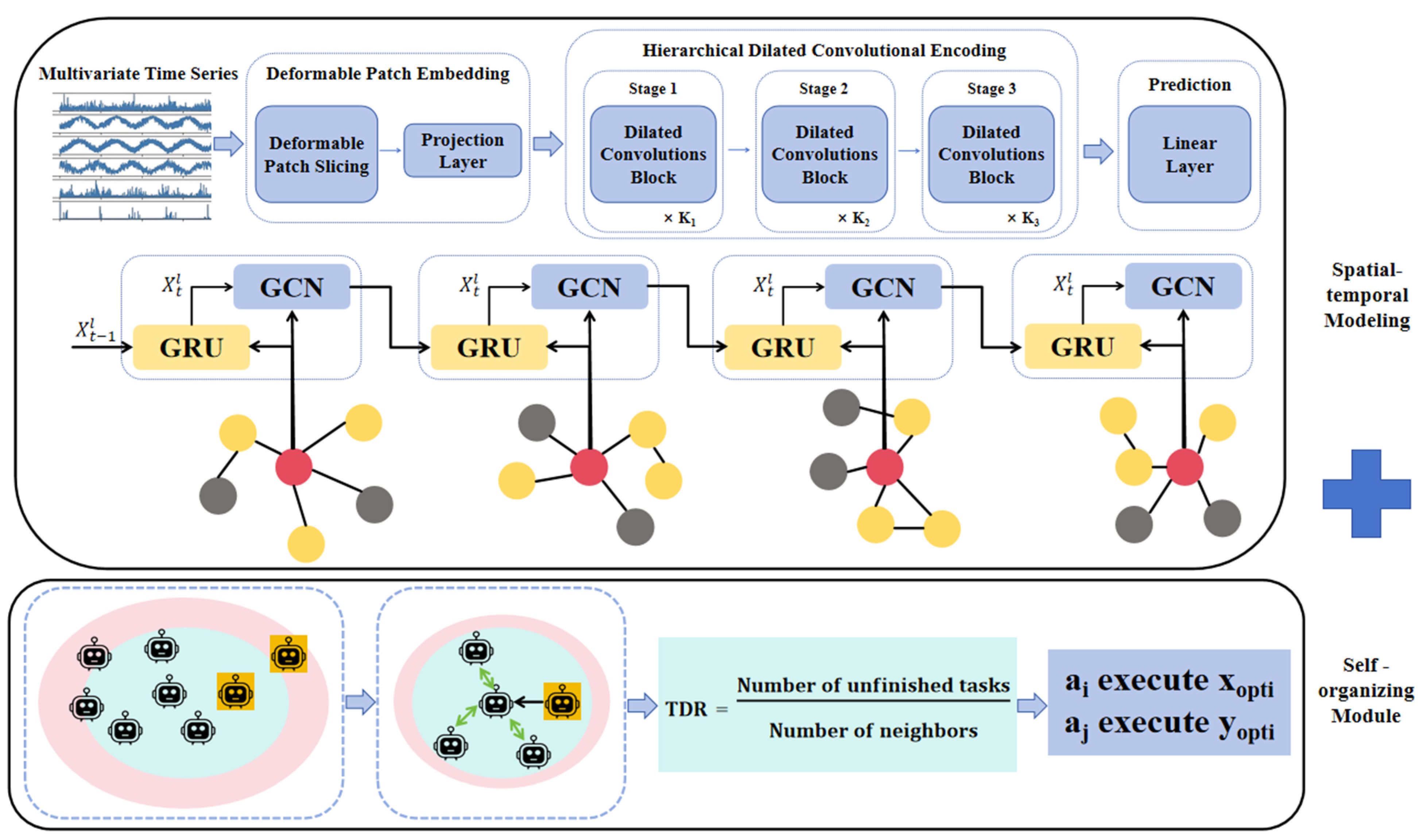
Based on this, the objective of this paper is to complete spatio-temporal modeling and accomplish complex resource allocation by utilizing the self-organization mechanism of intelligent clusters based on the trust model. The overall structure of the proposed approach is shown in Figure 1.

Our main contributions are as follows:

(1)

In time modeling, dilated convolution is adopted to capture the time trends of graph nodes. Its dilation rate grows exponentially with the depth of the layer, which enlarges the receptive field, enables effective processing of long time series data, alleviates the gradient explosion problem, and is conducive to parallel acceleration. In spatial modeling, a dual-view dynamic graph convolutional network architecture is innovatively proposed. The self-attention mechanism is utilized to calculate the intensity of spatial correlation among nodes, and a correlation matrix is introduced to mine the static and dynamic correlation information of the spatial layout of charging piles.

(2)

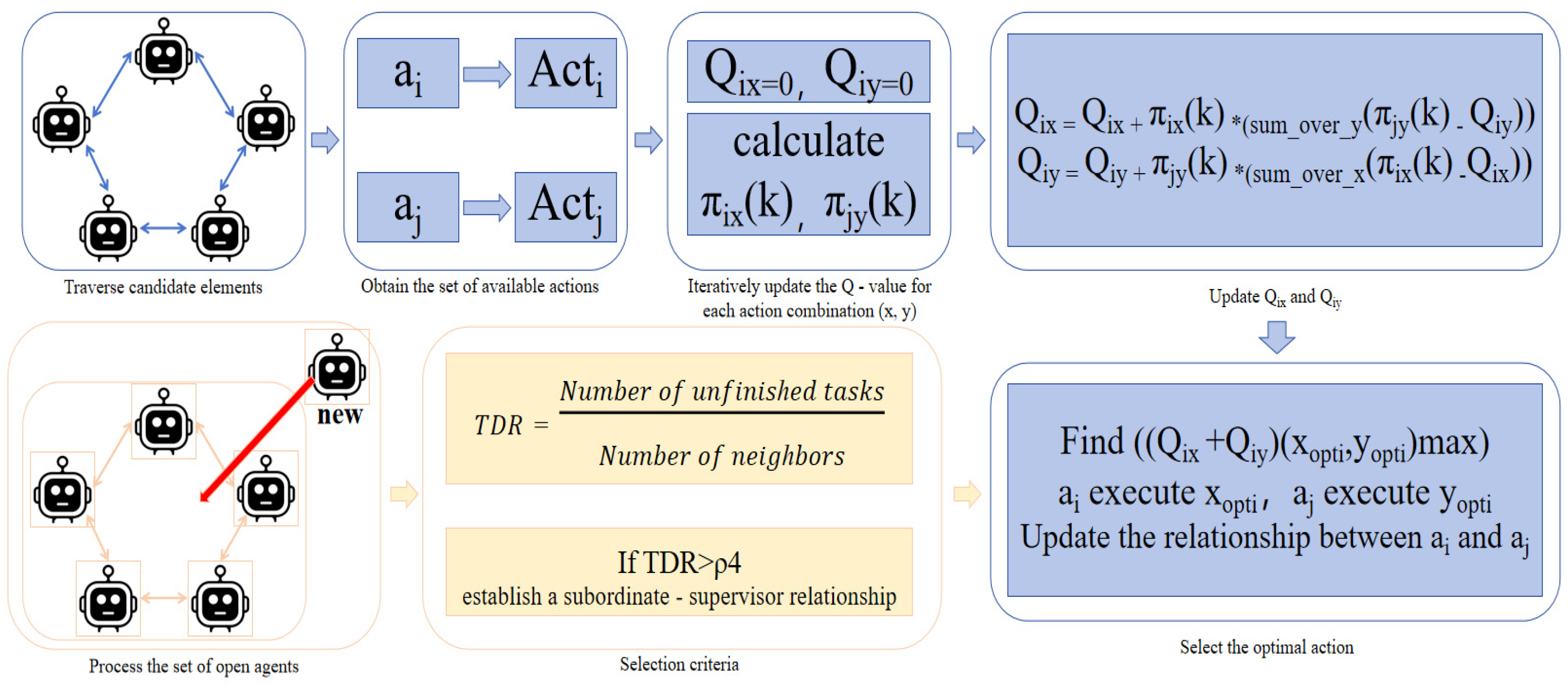
A composite self-organization mechanism is proposed. The trust model is integrated into the aspect of candidate selection, enabling agents to choose candidates by using not only their own experiences but also the opinions of other agents. An intelligent cluster Q-learning algorithm is developed, allowing agents to independently evaluate their rewards regarding the adaptation relationship. Compared with the relevant methods that currently only consider clear relationships, we also introduce weighted relationships into the self-organization mechanism to make it more suitable for dynamic environments.

(3)

By considering multiple EV charging piles as an intelligent cluster system and considering spatio-temporal data, EV mobility, and different charging modes, we conduct experiments with the EV charging demand prediction model. The results verify the effectiveness of the spatio-temporal self-organization prediction as it shifts the charging pile load from peak to valley, minimizing the peak–valley difference, enhancing microgrid security, and enabling resource optimization and intelligent scheduling. Moreover, compared with algorithms like MPC, DDQN, PPO, DDPG, and PSO in EV charging scheduling over five weeks based on occupancy and waiting time, our self-organization algorithm performs better. It has a 60% occupancy rate while others are lower, and a 0.20 h average waiting time shorter than others, demonstrating its superiority in optimizing charging resources and system efficiency.

2. Spatio-Temporal Modeling

2.1. Time Modeling Based on Dilated Convolution

In spatio-temporal modeling, an important task is to model the time correlation. Dilated convolution is adopted as the time convolution layer to capture the time trends of graph nodes. In particular, in the dilated convolution network, it is allowed to obtain an exponentially growing receptive field by increasing the depth of the network layer, thus effectively expanding the historical range for processing time series data. Specifically, the dilated convolution introduces a dilation rate on the basis of the causal convolution. By skipping some parts of the input, the filtering kernel can be applied to areas larger than the length of the filtering kernel itself. Moreover, the dilation rate grows exponentially with the layer depth, and therefore the receptive field also increases accordingly.

Suppose at node v_i, given a one-dimensional time series x ∈ R^H and a filtering kernel k ∈ R^K*, then the dilated convolution is defined as follows:

$$x_{dc}^{*}k[t]={\displaystyle \sum _{s=0}^{K^{*}}k}[s]x[t-d^{*}s]$$

(1)

Among them, *_dc is the dilated convolution operator, K^* is the size of the dilated convolution kernel, and d is the dilation factor. The value of d controls the skipping distance, that is, one input is selected for every d step.

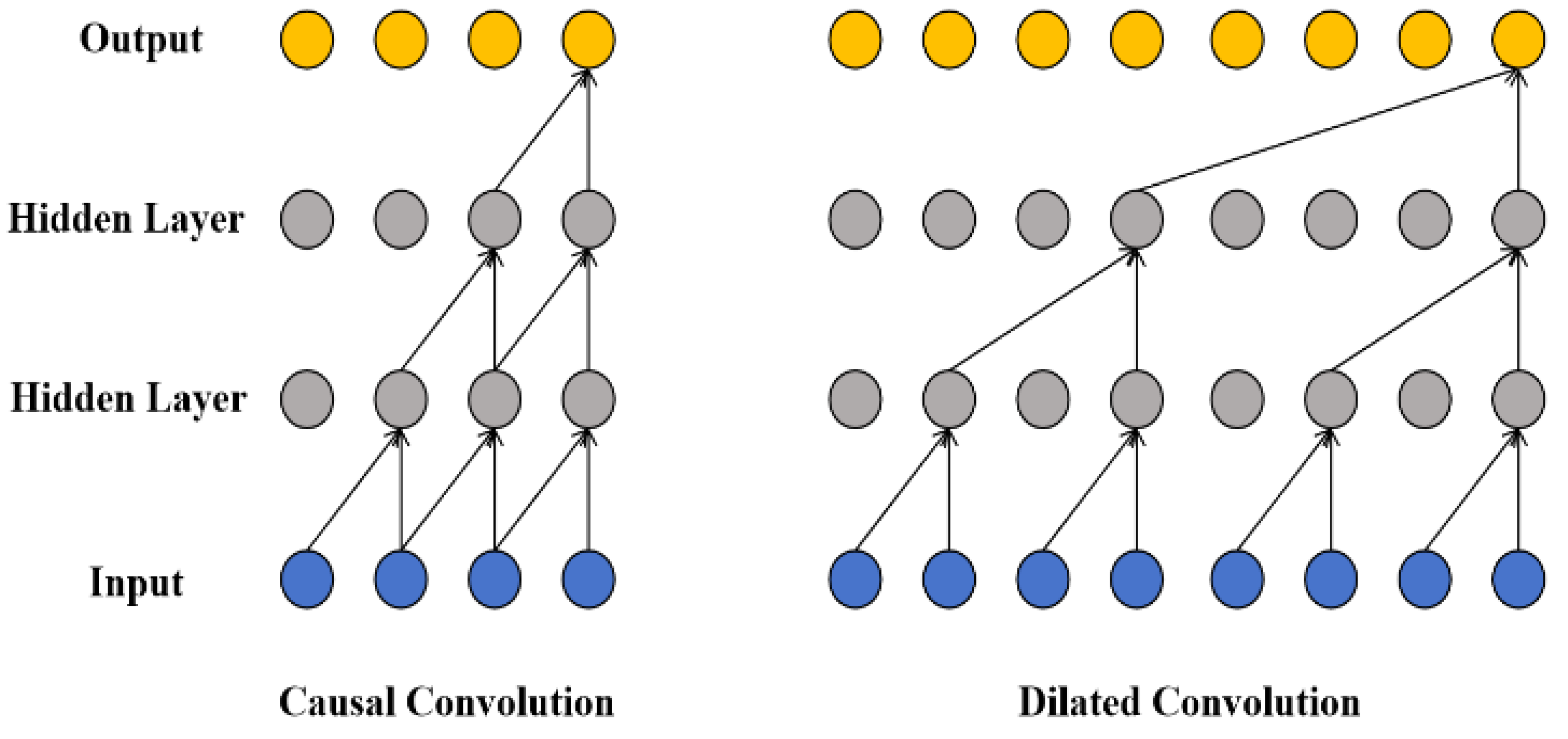
To describe the role of dilated convolution more clearly, we illustrate the causal convolution and the dilated convolution, as shown in Figure 2. In Figure 2, the receptive field of the convolution operation is increased by stacking multiple convolution layers. For the historical feature sequence of node vi in the given graph, with the same number of network layers, the receptive field of the causal convolution (as shown on the left in Figure 2) is significantly smaller than that of the dilated convolution (as shown on the right in Figure 2). Generally, in the dilated convolution layers, as the number of convolution layers increases, the dilation factor increases exponentially, and the receptive field of the model also increases exponentially. In Figure 2, the receptive field of the dilated convolution is expanded by 1 time, 2 times, and 4 times, respectively, at each layer. This enables the dilated convolution to capture the correlations among long sequence data by stacking network layers with a limited depth, thus effectively saving computing resources. Compared with the methods based on Recurrent Neural Network (RNN), it has obvious advantages. The dilated convolution can handle long time series data in a non-recursive manner. This non-recursive processing method is conducive to parallel acceleration. Meanwhile, the dilated convolution effectively alleviates the problem of gradient explosion.

The calculation of dilated convolution can be described by the following steps.

Define the convolution kernel and the dilation rate: Suppose the size of the convolution kernel is k × k, and the dilation rate is d. The dilation rate defines the spacing between elements in the convolution kernel; that is, d − 1 zeros are inserted between non-zero elements in the convolution kernel.

Calculate the size of the equivalent convolution kernel: The size k′ of the equivalent convolution kernel for the dilated convolution can be calculated by the following formula:

$$k^{\prime }=k+(k-1)\times (d-1)$$

(2)

Among them, k′ represents the size of the equivalent ordinary convolution kernel, k represents the size of the dilated convolution kernel, and d represents the dilation rate.

Calculation of the receptive field: For the receptive field RFi of the i-th layer and the size k′ of the equivalent convolution kernel, the recursive relationship of the receptive field of the next layer (deeper layer) is the following:

$$R{F}_{i+1} =R{F}_i +(k^{\prime }-1)\times S_i$$

(3)

Among them, Si represents the product of the strides of the i-th layer and all previous layers.

Convolution operation: In the actual convolution operation, the convolution kernel will slide over the input feature map. For each position, the non-zero elements in the convolution kernel perform a dot product operation with the corresponding elements on the feature map, and the results are summed up to obtain an element of the output feature map.

For EV resource scheduling, the time series data we deal with is closely related to the charging behaviors and arrival and departure times of vehicles, which are influenced by various factors such as user habits, traffic conditions, and grid load. Our innovation lies in customizing the parameters of dilated convolution, including the selection of dilation rates and kernel sizes, according to the characteristics of EV-related time series data. For example, we adjust the dilation rate based on the typical charging cycle patterns of different types of EVs, enabling the model to better capture the long-term trends in charging demands. This tailored approach allows us to accurately predict the future load of charging piles and optimize the resource allocation in real time. By doing so, we can not only improve the efficiency of EV charging but also enhance the stability of the power grid, which is a significant improvement compared to simply applying standard dilated convolution methods.

2.2. Spatial Modeling Based on Dynamic Graph Convolution

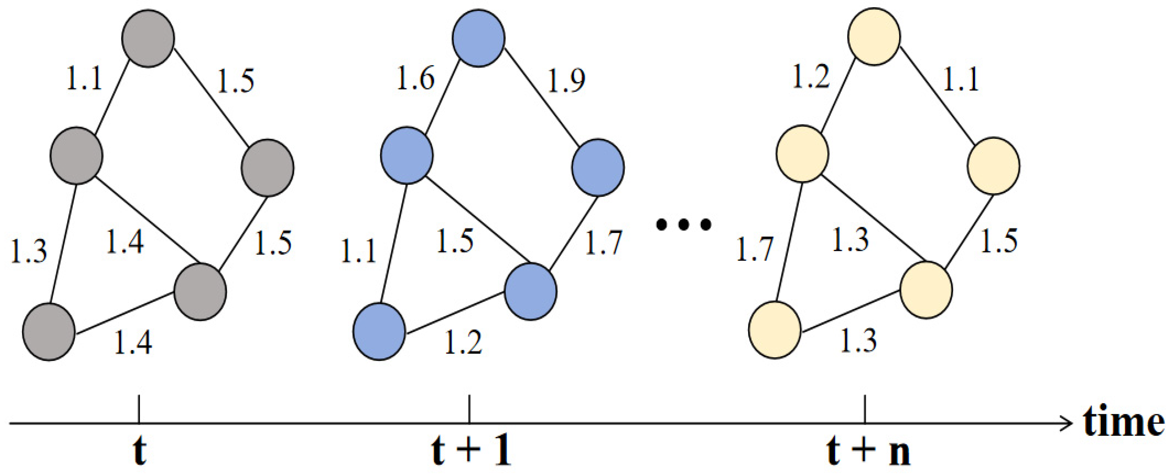
In the context of exploring the spatial layout of electric vehicle charging piles, since it can be abstracted into a graph structure composed of individual charging piles as nodes and the connection paths or the lines representing the potential influence ranges among them as edges, graph convolutional networks can be naturally applied to mine the pattern and feature information in the spatial layout of charging piles. On this basis, this paper innovatively proposes a dynamic graph convolutional network architecture from a dual perspective, which is committed to accurately learning the multiple and complex spatial correlations contained in the spatial distribution of charging piles, providing strong support for electric vehicle owners to charge quickly and for the efficient management of charging piles. Specifically, the original graph convolution learning process is shown as follows:

$$H_{l+1}=GCN(H_l)=\sigma (A{H}_{l}W)$$

(4)

Among them, H_l represents the input of the l-th graph convolutional layer, σ is the activation function, A is the adjacency matrix, and W is the learnable weight matrix. As shown in Figure 3, since the original graph convolutional model can only be used to learn the spatial correlation relationships in static graphs and cannot capture the dynamic spatial correlations among nodes in the actual road network, the original graph convolutional network cannot be directly applied to the learning of dynamic road networks.

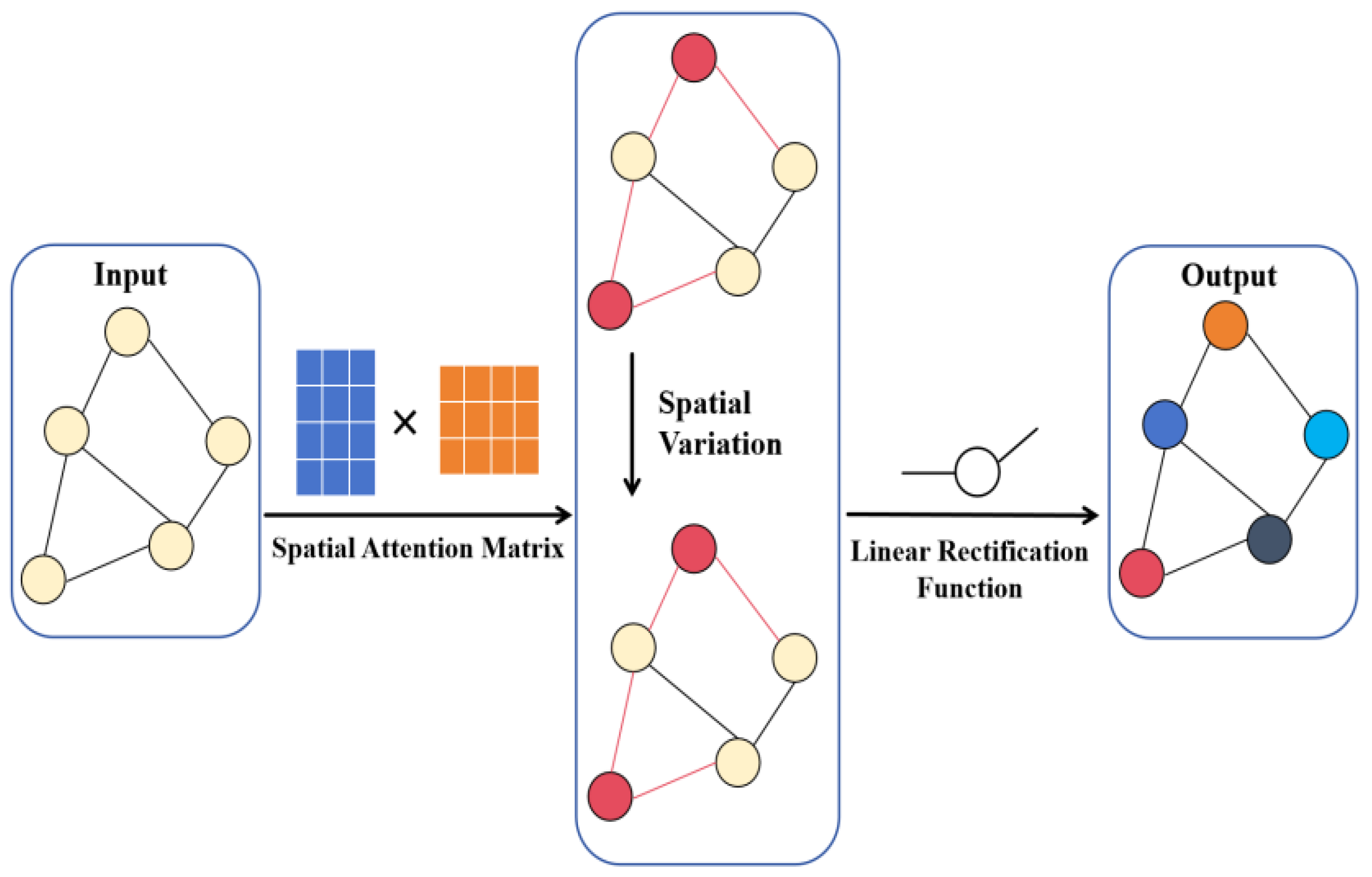
In order to capture the dynamic spatial correlations among nodes in the road network, this paper designs a dynamic graph convolution from a dual spatial perspective. It utilizes the self-attention mechanism to dynamically calculate the intensity of spatial correlations among nodes and adaptively adjust the connection relationships among nodes. Given the representations of nodes and the output Z_l of the multi-head attention of the time–local convolution, the calculation of the spatial attention correlation weight matrix is shown as follows:

$$S_{att}=max\left({\displaystyle \frac{Z_l{Z}_l^T}{\sqrt{d_{model}}}}\right)\in {ℝ}^{M\times M}$$

(5)

Among them, S_att(i,j) represents the intensity of the correlation between node i and node j. The larger the value of S_att is, the greater the intensity of the correlation between the nodes. The adjacency matrix A is adjusted through the spatial attention correlation weight matrix to obtain the output of the dynamic graph convolution module. The calculation formula of the dynamic graph convolution is shown as follows, and the construction steps of the dynamic graph convolution are shown in Figure 4. After performing the multi-head self-attention operation of time–local convolution on all road network nodes, the intermediate representation of the sequence Z_l^’ = (Z_l,t−m+1, Z_l,t−m+2, …, Z_l,t) is obtained, and with this as the input, the dynamic graph convolution calculation is carried out:

$$DGCN(Z_l)=\sigma ((A\odot S_{att})Z_{l}W)$$

(6)

Among them, ⊙ represents the Hadamard product. The spatial dynamic graph convolution directly uses the adjacency matrix A, only considering the single static structure of the traffic road network and ignoring the similar functional characteristics among nodes as well as the influence of dynamic traffic patterns. Therefore, the spatial structure matrix A^S and the dynamic correlation matrix A^D are introduced to capture the static spatial correlation and dynamic temporal similarity in traffic data, respectively. Based on the traffic graph matrices from a dual perspective, the spatial structure graph convolution module and the dynamic correlation graph convolution module are further constructed:

$$X_{l+1}^S=SDGCN(Z_l)=\sigma ((A^S\odot S_{att})Z_{l}W)$$

(7)

$$X_{l+1}^D=DDGCN(Z_l)=\sigma ((A^D\odot S_{att})Z_{l}W)$$

(8)

After the dynamic graph convolution from a dual spatial perspective, the operations of spatial structure graph convolution and dynamic correlation graph convolution are carried out, and the results of spatial structure graph convolution and dynamic correlation graph convolution are output. The spatial modeling based on dynamic graph convolution can capture the static spatial correlation relationships and the hidden temporal dynamic correlation relationships among the nodes of the road network, enabling the learned node representations to contain both static geographical spatial information and dynamic temporal semantic information, which can effectively mine the static spatial characteristics and dynamic temporal patterns in the spatial road network.

The spatial layout of charging piles is not just a static graph problem; it is intricately linked to real-time traffic flows, fluctuating charging demands, and the movement patterns of EVs. We have adapted the dynamic graph convolution to directly address these factors. By integrating real-time traffic data into the calculation of the spatial attention correlation weight matrix, the network can dynamically adjust to changing traffic conditions. For example, during peak traffic hours, the system can quickly identify charging piles in areas with high vehicle congestion and redistribute charging resources accordingly. The introduction of the spatial structure matrix and dynamic correlation matrix is specifically designed to capture the dual nature of EV charging scenarios: the static geographical layout of charging piles and the dynamic temporal variations in demand. This enables the model to predict not only where EVs are likely to seek charging but also when facilitating more efficient resource allocation. In contrast to standard graph convolution models, our approach does not just learn spatial relationships but actively optimizes the entire EV charging process, reducing waiting times for users and enhancing the overall utilization of charging infrastructure.

3. Composite Self-Organization Algorithm with Integrated Trust Model

3.1. Trust Model

Let T represent that the given agent considers the corresponding party to be trustworthy. $\theta =\{T,\neg T\}$ is the discrimination framework. The power set of $\theta$ is represented as $H^{\theta }=\{\varnothing ,\{T\},\{\neg T\},\{T\cap \neg T\},\theta \}$. There exists a general basic belief assignment, which is a function m:$H^{\theta }\to [0,1]$, where

$$\left\{\begin{array}{lll}m(\theta )=0\hfill & \hfill & \hfill \\ {\displaystyle \sum _{B{H}^{\theta }}m}(B)=1\hfill & \hfill & \hfill \end{array}\right.$$

(9)

$$m(\{T\})+m(\{\neg T\})+m(\{\theta \})+m(\{T\cap \neg T\})=1$$

The trust model is defined as a tuple.

$$T_j^i=\langle m_j^i(\{T\}),m_j^i(\{\neg T\}),m_j^i(\{\theta \}),m_j^i(\{T\cap \neg T\})\rangle ,$$

where i and j represent two different agents a_i and a_j. Each element in $T_j^i$ is described as follows:

• $m_j^i(\{T\})$ represents the degree to which agent a_i trusts agent a_j;
• $m_j^i(\{\neg T\})$ represents the degree to which agent a_i distrusts agent a_j;
• $m_j^i(\{\theta \})$ indicates the degree of uncertainty in agent a_i trustworthiness assessment of agent a_j. This case occurs when agent a_i lacks evidence about agent a_j. If agent a_i has no evidence at all, $m_j^i(\{\theta \})$ = 1; otherwise, $m_j^i(\{\theta \})$ < 1;
• $m_j^i(\{T\cap \neg T\})$ describes the degree of conflict in the trustworthiness assessment from agent a_i to agent a_j. An example of this situation is when agent a_i trusts agent a_j, but other agents providing feedback to a_i distrust agent a_j, causing agent a_i to be in a state of conflict.

Therefore, initially, the trust between any two agents is as follows: $T_j^i=\langle m_j^i(\{T\})=0,m_j^i(\{\neg T\})=0,m_j^i(\{\theta \})=1,m_j^i(\{T\cap \neg T\})=0\rangle$.

Trust is obtained through information exchange between agents. Suppose agent a_i is evaluating the trustworthiness of agent a_j, and agent a_j has allocated x resources to agent a_i. Agent a_i uses the concept of Quality of Service (QoS) to express its satisfaction with the services provided by agent a_j for each allocated resource task. Therefore, for x resources, there are x QoS values. QoS is within the range [0,1], and its calculation depends on the time taken to complete the resource allocation. For example, if agent a_j completes the resource allocation task for agent a_i on time, then the QoS for that resource is estimated as QoS = 1; otherwise, the QoS value will decrease over time.

3.2. Self-Organization Algorithm

The Algorithm 1 is designed to adapt the interactions between each pair of elements a_i and a_j (or related elements) based on their relationships within a given set of elements E. First, we determine the set of available actions for each element, which may depend on the current state between elements or the external environment. Next, we iterate over every possible action combination (x, y), where x is the action for a_i and y is the action for a_j (or vice versa). For each action combination, we initialize the accumulated utility functions Qix and Qiy to 0 and then update them by iterating over a predefined range of integers. In each iteration, we calculate π_ix(k) and π_jy(k), which represent the utility or probability of actions x and y at the specific iteration k, according to a given policy or model. To compute π_ix, we employ the Q-exploration method. If a certain condition is met (e.g., pji is less than k, where pji is a measure based on the current relationship), we update Qix and Qiy to reflect the expected impact of performing these actions on future states or relationships. After traversing all possible action combinations, we find the optimal action combination (x_opti, y_opti) that maximizes the total of Qix and Qiy, and let elements a_i and a_j (or the related elements) perform these actions accordingly. Subsequently, we update the relationship measure between the elements (e.g., μij) based on the executed actions, which may involve increasing or decreasing the strength of the relationship, depending on the effects of the actions and the system’s rules. In this way, the algorithm dynamically adapts to the relationships between elements and optimizes their interactions.

Algorithm 1: Demonstrates Our Q-learning Self-Organization Algorithm

Algorithm: RelationAdaptation(E)    For each a_i in E Candidates:    Act_i = get_available_actions(a_i)    Act_j = get_available_actions(a_j)    For each x in Act_i, y in Act_j:    Initialize Qix = 0, Qy = 0    For k = 0 to a predefined integer:    calculate π_ix(k) and π_jy(k)    if (pji < k):    Qix = Qix + π_ix(k) * (sum_over_y(π_jy(k) − Qiy))    Qiy = Qiy + π_jy(k) * (sum_over_x(π_ix(k) − Qix))    else:    End For    (x_opti, y_opti) = argmax_over_x_y(Qix + Qiy)    a_i takes action x_opti    a_j takes action y_opti    Update_relation_metric(a_i, a_j)    End For End Algorithm

After explaining the basic components of our self-organization mechanism, we now discuss how the mechanism handles an open set of agents. When a new agent a_j joins the network, it has no historical interactions with the existing agents in the network. Therefore, a_j cannot directly choose a candidate to form a relationship with. Generally, a_j prefers to connect to an existing agent a_i, especially one that has more unfinished resource allocation tasks, as it can gain rewards by completing those tasks, rather than connecting to agents with fewer unfinished tasks. At the same time, a_j dislikes connecting to an agent a_i that already maintains many neighbors, because the more neighbors a_i has, the fewer opportunities a_j will have to obtain information from a_i. Additionally, too many neighbors would put a heavy workload on a_i to maintain relationships with them. Therefore, the candidate selection for a_j is based on the ratio between the number of unfinished resource allocations and the number of neighbors (commonly referred to as the degree) for each existing agent, recorded as the TDR (Task-degree Ratio). If the TDR of a_i exceeds a predefined threshold ρ4, then a_j establishes a subordinate–supervisor relationship with a_i. In contrast, when an existing agent leaves, other agents can easily reorganize using our self-organization mechanism.

The Q-learning self-organization algorithm gradually approximates the optimal policy by iteratively updating the Q values without the need to construct a complex environment model. In each iteration, the immediate reward and the expected future reward are calculated based only on the current state and the chosen action, thereby reducing computational complexity. In terms of response time, a distributed decision-making architecture is employed, where each agent independently updates its Q values and makes decisions, enabling the system to respond quickly to environmental changes. Especially when dealing with large-scale intelligent cluster systems, this distributed decision-making mechanism can significantly reduce decision-making delays and improve the overall response speed of the system, as shown in the flow Figure 5 of the self-organizing algorithm.

4. Experiment

4.1. Self-Organizing Prediction Experiment on Spatio-Temporal Distribution

Due to the uncertainty and diversity of the charging demands and user behavior habits of electric vehicles in the future, the charging loads of large-scale electric vehicles will exhibit characteristics such as volatility, intermittence, and randomness in terms of time and space, which will lead to the shortage of power resources for charging piles. Therefore, accurately predicting the power demands of charging piles and reasonably allocating power resources have become the keys to improving charging efficiency and charging speed.

The main steps of the experiment in this paper are as follows. Firstly, consider the urgency of spatio-temporal resource allocation requirements, and determine the urgency of charging requirements through the Resource Urgency Index (RUI). Secondly, all charging piles dispatch electric vehicles according to different charging requirements instead of dispatching them as a whole. Finally, in order to prove the effectiveness of the proposed method in practical situations, two different electric vehicle charging methods are adopted for simulation, taking into account the uncertainty of electric vehicle charging behaviors. The results show that this method transfers the load demand from the peak period to the valley period through self-organizing the dispatching of electric vehicle charging, minimizes the total peak–valley load difference, and helps to improve the security and reliability of the microgrid.

During the process of charging resource allocation, the charging pile aggregator agent collects charging information to realize the charging dispatching of electric vehicles. When an electric vehicle is connected to the microgrid, the owner of the electric vehicle sets the charging information and sends it to the electric vehicle aggregator agent. This information includes the arrival time and departure time, the State of Charge (SOC) when the electric vehicle is connected to the microgrid, and the upper and lower limits of the SOC for the charging demand of the electric vehicle. Then, the arrival time and departure time of the electric vehicle are normalized into time slots. Then, the electric vehicle RUI is defined to distinguish whether the charging demand of the electric vehicle is urgent or not, and home charging modes are provided for electric vehicle owners. In the charging resource allocation model proposed in this paper, the charging state is a state variable used to reflect whether the electric vehicle is being charged in a certain time slot. The goal of the proposed self-organizing charging dispatching method is to minimize the peak-to-valley load difference in the microgrid.

The core optimization problem is to minimize the peak–valley load difference in the microgrid while ensuring that SOC requirements of electric vehicles are met. Let L_t denote the total load of the microgrid at time slot t, where t = 1, 2,…, 96. The peak–valley load difference ΔL is defined as the difference between the maximum load $L_{max}={\max }_t(L_t)$ and the minimum load $L_{min}={\min }_t(L_t)$ over all time slots.

The definition of RUI is based on SOC. The Resource Urgency Index for electric vehicle i, denoted as RUI_i, is defined as follows:

$$RU{I}_i={\displaystyle \frac{SO{C}_{min,i}-SO{C}_{i,t_{arrival,i}}}{SO{C}_{max,i}-SO{C}_{min,i}}}$$

(10)

SOC_min,i: Minimum State of Charge for vehicle i. This is the lowest level of charge that vehicle i can safely operate at or the threshold below which it is considered critically low on charge.

SOC_i,tarrival,i: State of Charge of vehicle i at the time of its arrival, denoted as tarrival,i. It indicates the amount of charge the vehicle has when it arrives at the charging station.

SOC_max,i: Maximum State of Charge for vehicle i. This is the highest level of charge that vehicle i’s battery can hold.

When RUI_i is close to 1, it indicates that the electric vehicle has an urgent charging requirement, as its current State of Charge is far from the minimum required level. Conversely, when RUI_i is close to 0, the charging requirement is less urgent. This index helps in differentiating the charging urgency of electric vehicles, which is crucial for the self-organizing charging dispatching process to effectively transfer load demand from peak to valley periods and achieve the optimization goal.

Considering the charging habits of electric vehicle owners, the conventional charging mode of electric vehicles is the home charging mode. Under this mode, electric vehicle owners start charging when they get home from work and finish charging when they are ready to go to work. The arrival time and departure time of electric vehicles follow a normal distribution.

4.2. Self-Organization Results and Comparative Analysis

During the dispatching process, the dispatching plan is usually executed in units of time periods to improve the execution efficiency. The dispatching time is divided into several time periods. In the proposed electric vehicle charging dispatching model, a day is discretized into 96 time slots, and each time slot has a length of 15 min.

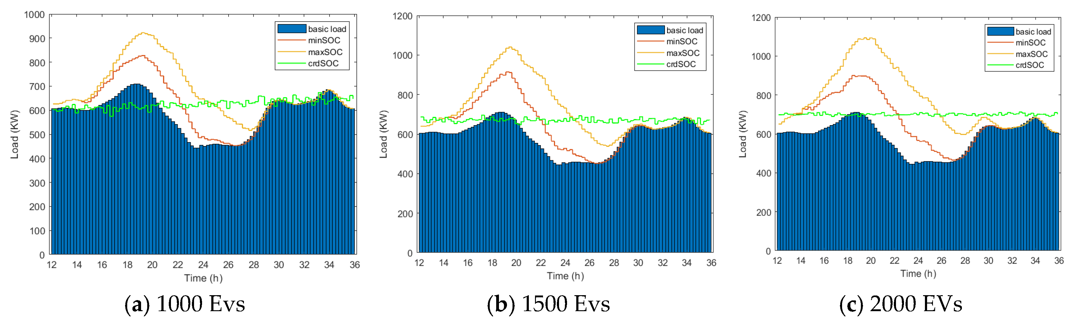
In the home charging mode, the simulation results of the charging pile charging dispatching under three different charging methods are shown in Figure 6. In each figure, three different charging dispatching scenarios are adopted. For the non-self-organizing charging dispatching plan, electric vehicles start charging from the arrival time slot and remain in the charging state until the departure time slot or until the time slot meets the owner’s maximum SOC requirement.

For electric vehicles with urgent charging requirements, some electric vehicles have too short a charging time, and the non-self-organizing charging strategy cannot ensure that the minimum SOC requirement of electric vehicles is met in such urgent situations. However, the self-organizing charging dispatching method can handle urgent charging situations.

For electric vehicles with slow charging requirements, the self-organizing environment ensures that when electric vehicles are disconnected from the microgrid, the SOC should be between the maximum and minimum values. Therefore, in the self-organizing situation, the total charging power of electric vehicles in the microgrid is lower than that of the non-self-organizing charging plan that meets the maximum SOC requirement and higher than that of the non-self-organizing charging plan that meets the minimum SOC requirement. As shown in Figure 6, the charging curve under the self-organizing mode is smoother than the charging curves under the two non-self-organizing modes.

Table 1. The impact of self-organizing charging methods on peak shaving and valley filling for home charging.

Number of EV		1000	1500	2000
Change in peak value	UC (max SOC)	−21.86%	−31.87%	−36.77%
	UC (min SOC)	−15.69%	−23.97%	−28.56%
Change in valley value	UC (max SOC)	+11.33%	+11.09%	+10.52%
	UC (min SOC)	+30.25%	+31.76%	+32.51%
Change in range	UC (max SOC)	−75.86%	−84.72%	−90.37%
	UC (min SOC)	−77.21%	−83.26%	−89.66%
Change in variance	UC (max SOC)	−92.12%	−95.24%	−98.71%
	UC (min SOC)	−92.91%	−95.42%	−97.91%

compares the impact of the self-organizing charging mode on peak shaving and valley filling in home charging.

Compared with the two non-self-organizing charging dispatching methods, the self-organizing charging dispatching method can reduce the peak value, range, and variance of the total load. In addition, in order to compare the effects of the self-organizing charging dispatching method under different circumstances, we will compare the self-organizing charging dispatching method and the non-self-organizing charging dispatching method from three aspects.

Compared with the non-self-organizing charging dispatching method that meets the maximum SOC requirement, for 1000, 1500, and 2000 electric vehicles, the peak values of the self-organizing charging dispatching method are reduced by 21.86%, 31.87%, and 36.77%, respectively. Moreover, compared with the non-self-organizing charging dispatching method that meets the minimum SOC requirement, the self-organizing charging dispatching method can reduce the peak values by 15.69%, 23.97%, and 28.56%, respectively.

The adoption of the self-organizing charging dispatching method can reduce the total load ranges of the non-self-organizing charging dispatching that meets the maximum SOC requirement by 75.86%, 84.72%, and 90.37%, respectively. Similarly, the ranges of the non-self-organizing charging dispatching that meets the minimum SOC requirement can be shortened by 77.21%, 83.26%, and 89.66%, respectively.

Unlike the non-self-organizing charging dispatching method that meets the maximum State of Charge requirement, when the self-organizing charging dispatching method is adopted, under three different numbers of electric vehicles, the variances of the total load are reduced by 92.12%, 95.24%, and 98.71%, respectively. Meanwhile, the variances of the non-self-organizing charging dispatching method that meets the minimum SOC requirement can be reduced by 92.91%, 95.42%, and 97.91%, respectively.

4.3. Comparison of Similar Algorithms

In the field of electric vehicle charging scheduling, the performance of algorithms plays a crucial role in optimizing the utilization of charging resources and improving the overall efficiency of the charging system. This section will conduct a comprehensive comparison between the self-organizing charging scheduling algorithm and five other commonly used algorithms, namely MPC, DDQN, PPO, DDPG, and PSO, based on two key performance indicators: occupancy rate and average waiting time. The comparison period is five consecutive weeks, in order to examine the performance of these algorithms from a long-term and stable perspective.

Comparison of occupancy rates

The occupancy rate is an important indicator reflecting the utilization efficiency of charging facilities. A higher occupancy rate means that charging resources are utilized more effectively, which helps to maximize the return on investment in charging infrastructure.

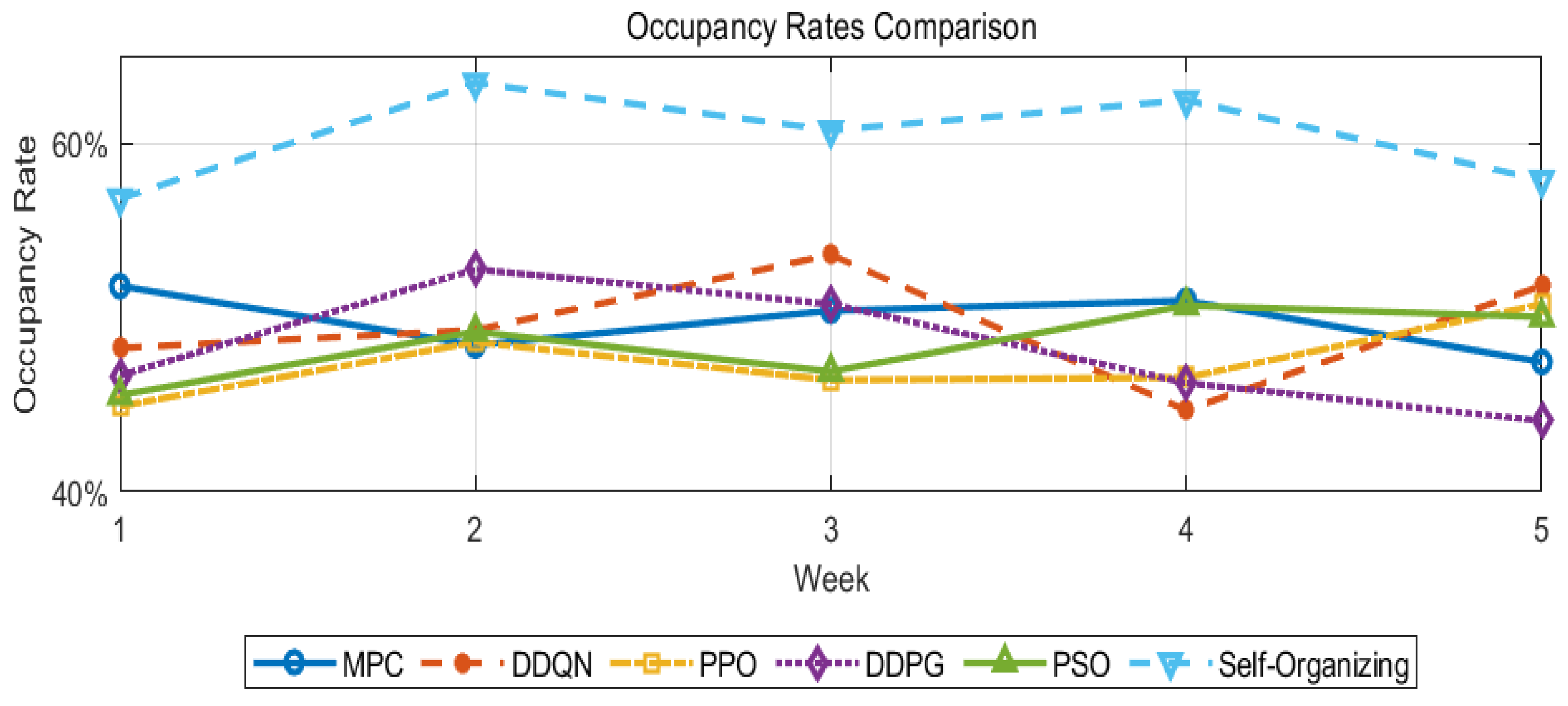
During the five-week comparison period, the self-organizing algorithm demonstrated excellent performance in terms of the occupancy rate. As shown in Figure 7, the occupancy rate of the self-organizing algorithm remained stable at around 60%. This stable and relatively high occupancy rate benefits from the self-regulating and self-optimizing characteristics of the self-organizing algorithm. It can dynamically coordinate the charging plans of electric vehicles based on various factors such as the arrival and departure times of vehicles, SOC requirements, and the real-time load of the microgrid.

In sharp contrast, the other five algorithms performed relatively poorly in terms of the occupancy rate.

MPC is an algorithm that uses a receding-horizon optimization approach. It randomly allocates charging time slots to EVs. In the graph, its average occupancy rate lingers around 50%. Its allocation method fails to adequately account for vehicle charging needs and resource availability, leading to suboptimal charging facility utilization.

DDQN, an improvement over traditional DQN, aims to reduce over-estimation bias. It prioritizes serving specific EV types, like high-priority user vehicles or those with urgent charging needs. However, as shown in the data, its average occupancy rate is merely about 49%. While it is considered a priority, it lacks a holistic coordination mechanism for all vehicles, causing non-prioritized vehicles to underutilize charging resources during off-peak hours.

PPO is designed to improve the sample efficiency of policy gradient methods. In the context of EV charging scheduling, it does not perform optimally in terms of occupancy rate. Its average occupancy rate is relatively low, as it does not seem to adapt well to the dynamic nature of EV charging demands, perhaps due to its focus on policy optimization rather than real-time demand-driven resource allocation.

DDPG is an actor-critic algorithm for continuous action spaces. In the occupancy rate comparison, it performs poorly, with an average occupancy rate that does not reach the levels of the self-organizing algorithm. It likely struggles to handle the complex, multi-factor environment of EV charging scheduling, failing to efficiently allocate resources to maximize occupancy.

PSO is inspired by the social behavior of bird flocking or fish schooling. In the case of EV charging, its average occupancy rate is not high. It may become trapped in local optima while searching for the best charging schedule, resulting in inefficient use of charging resources and a lower occupancy rate.

Comparison of average waiting times

The average waiting time is another key indicator that directly affects the charging experience of electric vehicle users. A shorter average waiting time means that electric vehicle owners do not have to wait long for their vehicles to be charged, improving the convenience of using electric vehicles.

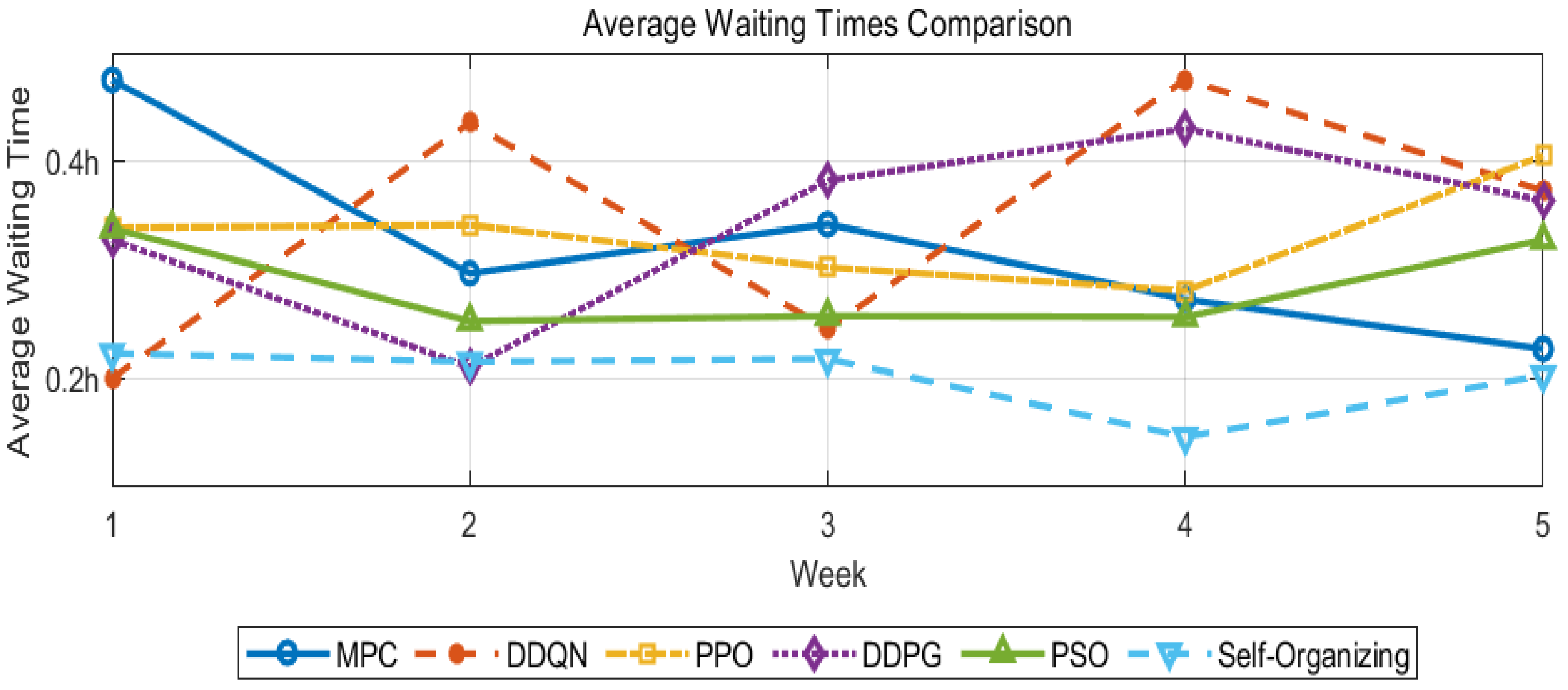
The self-organizing algorithm performs outstandingly in reducing the average waiting time. As shown in Figure 8, within five weeks, the average waiting time of the self-organizing algorithm has been stable at around 0.20 h. This benefits from the algorithm’s ability to predict and optimize the charging process in advance. By analyzing historical charging data and real-time vehicle information, the self-organizing algorithm can efficiently arrange the charging sequence and time, minimizing the vehicle waiting time to the greatest extent.

In contrast, the average waiting times of the other five algorithms are relatively long.

In electric vehicle charging scheduling, the average waiting time of MPC is about 0.35 h, and it has the problem of low efficiency in handling dynamic demand. The average waiting time of DDQN is approximately 0.32 h. Uneven vehicle service leads to a long overall waiting time. PPO has an average waiting time of around 0.35 h, and its FCFS-like characteristics cause scheduling inefficiency. DDPG has an average waiting time of roughly 0.38 h, and suboptimal scheduling decisions result in unreasonable waiting times. For PSO, the average waiting time is about 0.29 h, and its scheduling method disrupts charging while failing to optimize the waiting time effectively.

In conclusion, through the comparison of occupancy rates and average waiting times over five consecutive weeks, it is evident that the self-organizing algorithm outperforms the other five algorithms, namely MPC, DDQN, PPO, DDPG, and PSO, in terms of performance. The self-organizing algorithm can achieve both a high occupancy rate and a short average waiting time, mainly due to its adaptive intelligent scheduling mechanism. It can comprehensively consider various factors in the charging process, such as the arrival and departure times of vehicles, State-of-Charge requirements, and the real-time load of the microgrid, and make optimal decisions, thereby improving the utilization efficiency of charging resources and the charging experience of electric vehicle users.

4.4. Ablation Experiment of the Trust Model

In order to comprehensively evaluate the influence of the trust model in the composite self-organization algorithm on the performance of the overall system, an ablation experiment was carried out. The experiment compared the full model with the trust model and a baseline model without the trust model.

The experimental environment was consistent with the previous electric vehicle charging scenario experiments. The charging behaviors of electric vehicles followed the home charging mode, with arrival and departure times following a normal distribution. The charging process considered factors such as SOC of electric vehicles and RUI.

For the full model with the trust model, the trust model was integrated into the candidate selection process of the self-organization algorithm as described in Section 3.1. Agents would choose partners based on both their own experiences and the opinions of other agents, which were determined by the trust values calculated in the trust model.

The baseline model without the trust model removed the trust-based candidate selection mechanism. In the self-organization algorithm of the baseline model, agents selected partners only based on their own available actions and a simple rule-based method, without considering the trust relationship among agents.

Three key performance metrics were selected for comparison: peak–valley load difference, average waiting time, and occupancy rate. These metrics were crucial for evaluating the effectiveness of the charging scheduling algorithm and the performance of the overall system.

As shown in

Table 2. Comparison of performance metrics between the full model and the baseline model.

Performance Metrics	Full Model with Trust Model	Baseline Model Without Trust Model
Peak–Valley Load Difference (Reduction Percentage)	90.37% (for 2000 EVs)	72.19%
Average Waiting Time (h)	0.20	0.30
Occupancy Rate	60%	50%

, in terms of the peak–valley load difference, the full model with the trust model achieved a significantly greater reduction. The trust model helped agents make more rational cooperation decisions, which, in turn, optimized the charging scheduling and effectively balanced the load between peak and valley periods.

Regarding the average waiting time, the full model with the trust model had a shorter average waiting time. The trust-based partner selection mechanism enabled better coordination among agents, ensuring that electric vehicles could be charged more efficiently and reducing the overall waiting time.

For the occupancy rate, the full model with the trust model also outperformed the baseline model. The trust model promoted more effective resource allocation, allowing charging facilities to be utilized more fully and thus increasing the occupancy rate.

In conclusion, through this ablation experiment, it can be clearly seen that the trust model in the composite self-organization algorithm plays a crucial role in optimizing system performance. It effectively improves the charging scheduling, reduces the peak–valley load difference, shortens the average waiting time, and increases the occupancy rate, providing strong support for the efficient operation of the electric vehicle charging system.

5. Summary and Prospect

This paper focuses on the spatio-temporal resource allocation problem in intelligent cluster systems and proposes innovative solutions with remarkable achievements. In spatio-temporal modeling, the time modeling using dilated convolution and the spatial modeling with dual-perspective dynamic graph convolution provide a solid support for data processing. The combination of the trust model and the self-organizing algorithm in the composite self-organizing mechanism effectively enhances resource allocation efficiency and system adaptability. Through experiments in the electric vehicle charging scenario, the proposed method demonstrates excellent performance in optimizing charging dispatching, balancing peak and valley loads, and ensuring the stable operation of the microgrid. Notably, a comprehensive comparison experiment was conducted, which further validated the superiority of our method over other commonly used algorithms.

However, there is room for improvement. Despite incorporating stochastic behavior, our simulation assumes near-perfect info and comms, lacking models for agent dropout, delays, and failures, with no noisy/partial-info results. In future work, we will explore more complex scenarios like traffic and logistics, explicitly acknowledge this limitation in the discussion/conclusion, and aim to run an extra experiment with perturbed/missing data for robustness. Optimizing performance, scalability, and efficiency, and improving resource allocation and utilization remain our goals.