An Improved Finite-Set Predictive Control for Permanent Magnet Synchronous Motors Based on a Neutral-Point-Clamped Three-Level Inverter

Abstract

Numerous voltage vectors exist in a neutral-point-clamped (NPC) three-level inverter. Traditional three-level model predictive control incurs a heavy online computational burden. This paper proposes a model predictive torque control strategy for NPC three-level inverters with permanent magnet synchronous motor systems. First, the relationship among the stator flux linkage vector position, the torque–flux linkage increment, and the stator flux linkage variation is analyzed. Then, the candidate voltage vector sector is determined, and the candidate voltage vectors are selected from it. Meanwhile, the direction of the load current flowing to the neutral point and the voltage difference between the upper and lower capacitors are evaluated. As a result, redundant small vectors are effectively selected, reducing the number of candidate voltage vectors to six and avoiding the computation of all possible vectors. The experimental results from an NPC three-level inverter–permanent magnet synchronous motor system verify that this strategy significantly reduces the computational complexity and provides excellent dynamic and steady-state performance.

1. Introduction

PMSMs are characterized by a simple structure, high power density, high efficiency, and a high torque-to-inertia ratio. They are widely used in high-precision machine tools, traction drives, and elevator systems [1,2,3,4]. When the same DC power supply is used at the same frequency, three-level inverters exhibit lower voltage stress, higher output voltage quality, and lower switching losses than conventional two-level inverters [5]. Consequently, PMSM systems fed by neutral-point-clamped (NPC) three-level inverters are widely applied in high-voltage and high-power motor drive applications [6,7,8,9,10].

Vector control (VC) can achieve dynamic characteristics and control precision comparable to those of DC motors, but it suffers from drawbacks such as complex coordinate transformations and a heavy reliance on motor parameters [11]. The direct torque control (DTC) strategy [12] selects voltage vectors for control through hysteresis comparisons of the torque and flux linkage, which results in significant torque ripple and suboptimal control performance. Model predictive control (MPC) [13] is another high-performance motor control strategy following VC and DTC. MPC relies on the system’s mathematical model to predict future output states, optimizes control actions based on a cost function, and thereby enhances control flexibility. Finite control set MPC (FCS-MPC) leverages the discrete nature of inverters by performing predictive calculations only on the finite set of voltage vectors output by the inverter. This simplifies the algorithm and makes it more practical. The application of MPC to motor drive systems has thus become a current research focus [14,15,16].

Model predictive torque control (MPTC) [17] integrates the basic voltage vectors generated by the inverter with control objectives, handles system constraints, and achieves precise torque regulation. When MPTC is applied to a motor speed regulation system driven by an NPC three-level inverter, the increased number of voltage vectors enables better fulfillment of control requirements such as torque gradation and flux linkage regulation. This results in reduced torque ripple and smoother speed performance. However, the larger set of candidate vectors significantly increases the computational burden during vector selection, leading to degraded dynamic performance. In FCS strategies, research aimed at reducing the number of candidate vectors, decreasing the computational load, and enhancing system dynamic performance has been conducted to alleviate the computational burden of MPC algorithms [18,19]. In Ref. [18], a branch-and-bound algorithm was adopted to prune suboptimal switching sequences, thereby improving the computational efficiency of predictive torque control. In Ref. [19], a modified sphere decoding algorithm was employed to enhance system performance. Reference [15] addresses the least squares problem for linear systems, reducing the computational complexity and load. In references [20,21], the number of possible switching sequences is minimized to alleviate the computational burden of PTC algorithms. Numerous published strategies for reducing the computational load and simplifying predictive control algorithms include sector partitioning strategies [22], the selection of adjacent voltage vector candidate sets [23], modified switching algorithms [24], dual-vector-based approaches [25], graphical algorithms [26], efficient FPGA implementations [27], and deadbeat (DB) optimization concepts [28].

In predictive control, the design of the cost function is critical. The weighting coefficients are defined as the proportions that the constraints for each control objective occupy in the cost function of model predictive control. The tuning of weighting coefficients significantly impacts the overall control performance of the system. However, this tuning process is highly complex and lacks strict mathematical guidelines. Eliminating weighting coefficients has thus become a research focus. In [29], various control objectives are converted using the deadbeat. The dimensions of torque and flux linkage are transformed into voltage vectors. Optimal control is then performed. In [30], torque variations and flux linkage variations are equivalently transformed into stator flux linkage. Voltage vectors are selected based on the torque variation and the angular position of the stator flux linkage. The selected vectors are then equivalently converted into stator flux linkage for cost-function optimization. This method cannot precisely represent the requirement for torque variation. In [31], the torque slope is defined as an expression with respect to the bus voltage. A graph is established to illustrate the relationship between the torque slope and the change in the voltage phase angle between consecutive time instants. A candidate sector of voltage vectors is constructed based on the previous voltage vector and the torque variation. However, flux linkage constraints are not imposed, and speed fluctuations are observed. Inverters are inherently subject to neutral-point voltage imbalance issues [32]. A neutral-point voltage control term may be added to the evaluation function. This term is used to satisfy the operating requirements of NPC three-level inverters. In reference [33], the vector switching sequence is adjusted, and redundant small vectors are inserted into the switching sequence to resolve the neutral-point voltage issue. These solutions are implemented at the modulation strategy level and are relatively complex to implement in motor control.

To address the aforementioned issues, a finite-set predictive torque control based on stator flux linkage observation is proposed. A spatial flux linkage sector is established, and the stator flux linkage position at the previous time step is observed. An appropriate candidate vector is then selected using torque and flux linkage hysteresis loops. This method effectively reduces computational complexity while reasonably constraining the torque and flux linkage requirements. The flow direction of the neutral-point current and the voltage difference between the upper and lower capacitors are utilized to select a small vector that balances the neutral-point potential. This approach not only reduces computational complexity but also eliminates the need for tuning the weight coefficient associated with the neutral-point voltage term in the cost function.

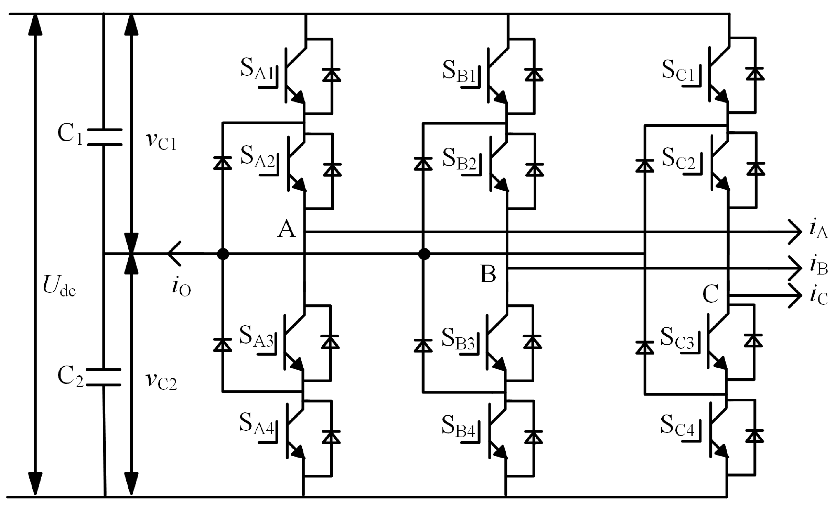
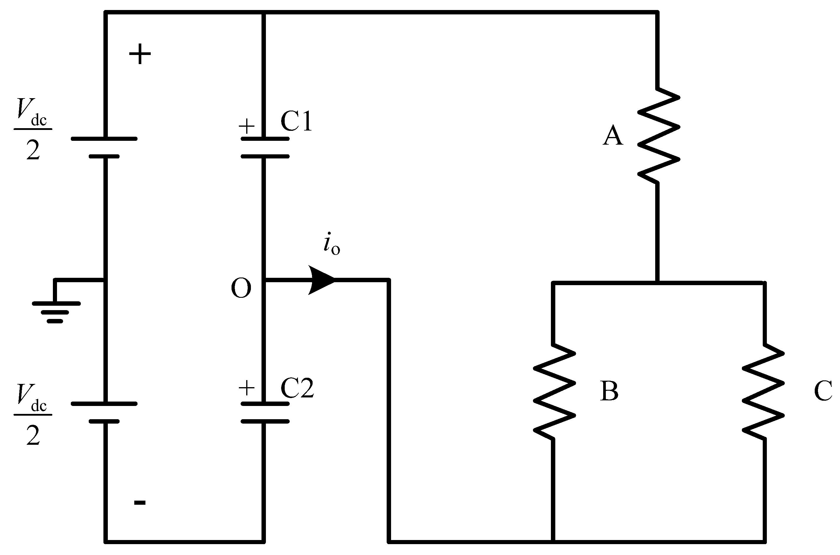
2. NPC Three-Level Inverter Structure

The NPC three-level inverter consists of 2 DC-side capacitors, 12 power switches, and 18 power diodes, as shown in Figure 1. The four power switches on each phase leg of the inverter control the switching between three voltage levels: P, O, and N. When S_x1 and S_x2 are on, it is the P state, and the output is U_dc/2; when S_x2 and S_x3 are on, it is the O state, and the output is 0; when S_x3 and S_x4 are on, it is the N state, and the output is −U_dc/2. S_n denotes the corresponding switch state for each phase, where S_n ∈ {1, 0, −1}, n ∈ {A, B, C}. S_A, S_B, and S_C represent the switching states of the three phases of the inverter. The relationship between S_A, S_B, and S_C and the switch states S_x1–S_x4 for each phase is represented as follows:

$$\left\{\begin{array}{l}{S}_{\mathrm{A}}=S_{\mathrm{A}1}+S_{\mathrm{A}2}-1\\ S_{\mathrm{B}}=S_{\mathrm{B}1}+S_{\mathrm{B}2}-1\\ S_{\mathrm{C}}=S_{\mathrm{C}1}+S_{\mathrm{C}2}-1\end{array}\right.$$

(1)

The three-phase bridge leg can generate 27 vectors, as shown in Figure 2. Based on the magnitude of the vectors, the voltage vectors can be classified into four categories: large vectors, medium vectors, small vectors, and zero vectors. The magnitude of the small vectors is U_dc/3, the magnitude of the medium vectors is √3U_dc/3, and the magnitude of the large vectors is 2U_dc/3.

3. Predictive Control Algorithm for PMSM

The mathematical model of the surface-mounted permanent magnet synchronous motor is established and discretized. The voltage, flux linkage, and electromagnetic torque equations of the PMSM are obtained, as shown in Equations (2)–(4):

$$\left\{\begin{array}{l}{u}_{\mathrm{d}}=R_{\mathrm{s}}{i}_{\mathrm{d}}+L_{\mathrm{d}}{\displaystyle \frac{\mathrm{d}{i}_{\mathrm{d}}}{\mathrm{d}t}}-{\omega }_{\mathrm{e}}{L}_{\mathrm{q}}{i}_{\mathrm{q}}\\ u_{\mathrm{q}}=R_{\mathrm{s}}{i}_{\mathrm{q}}+L_{\mathrm{q}}{\displaystyle \frac{\mathrm{d}{i}_{\mathrm{q}}}{\mathrm{d}t}}+{\omega }_{\mathrm{e}}(L_{\mathrm{d}}{i}_{\mathrm{d}}+{\psi }_{\mathrm{f}})\end{array}\right.$$

(2)

$$\left\{\begin{array}{l}{\psi }_{\mathrm{d}}=L_{\mathrm{d}}{i}_{\mathrm{d}}+{\psi }_{\mathrm{f}}\\ {\psi }_{\mathrm{q}}=L_{\mathrm{q}}{i}_{\mathrm{q}}\end{array}\right.$$

(3)

$$T_{\mathrm{e}}={\displaystyle \frac{3}{2}}{p}_{\mathrm{n}}({\psi }_{\mathrm{d}}{i}_{\mathrm{q}}-{\psi }_{\mathrm{q}}{i}_{\mathrm{d}})$$

(4)

where u_d, u_q, i_d, i_q, ψ_d, ψ_d, and ψ_q represent the components of the stator voltage vector u_s, the stator current vector is i_s, and the stator flux linkage vector ψ_s is along the d and q axes; T_e is the electromagnetic torque; ψ_f is the permanent magnet flux linkage; θ_r is the electrical angle of the flux linkage vector; ω_e = dθ_r/dt is the electrical angular speed of the rotor; R_s is the stator resistance; L_d and L_q are the direct and quadrature axis inductances; T_s is the control period; and p_n is the number of pole pairs of the motor [11,12].

For the stator current along the d-axis and q-axis at the next time step, i_d^k+1 and i_q^k+1 are predicted by discretizing Equations (2) and (3) using the first-order Euler method:

$$\left\{\begin{array}{l}{i}_{\mathrm{d}}^{k+1}={\displaystyle \frac{\left(u_{\mathrm{d}}^k-R_{\mathrm{s}}{i}_{\mathrm{d}}^k+L_{\mathrm{q}}{\omega }_{\mathrm{e}}{i}_{\mathrm{q}}^k\right)T_{\mathrm{s}}}{L_{\mathrm{d}}}}+i_{\mathrm{d}}^k\\ i_{\mathrm{q}}^{k+1}={\displaystyle \frac{\left(u_{\mathrm{q}}^k-R_{\mathrm{s}}{i}_{\mathrm{q}}^k-L_{\mathrm{d}}{\omega }_{\mathrm{e}}{i}_{\mathrm{d}}^k-{\omega }_{\mathrm{e}}{\psi }_{\mathrm{f}}\right)T_{\mathrm{s}}}{L_{\mathrm{q}}}}+i_{\mathrm{q}}^k\end{array}\right.$$

(5)

where u_d^k and u_q^k are the components of the motor’s voltage vector along the d-axis and q-axis at time k, and ω_e is the rotational speed at the current sampling period kT_s. Since the mechanical constant of the motor is much larger than the electrical constant, it is assumed that the speed does not change over the entire control period, i.e., ω_e^k+1 = ω_e^k.

Based on the predicted current values i_d^k+1 and i_q^k+1, for the stator flux linkage components ψ_d^k+1 and ψ_d^k+1, ψ_q^k+1 along the d-axis and q-axis at the end of the control period can be predicted using the following equation:

$$\left\{\begin{array}{l}{{\psi }_{\mathrm{d}}}^{k+1}=L_{\mathrm{d}}{i_{\mathrm{d}}}^{k+1}+{\psi }_{\mathrm{f}}\\ {{\psi }_{\mathrm{q}}}^{k+1}=L_{\mathrm{q}}{i_{\mathrm{q}}}^{k+1}\end{array}\right.$$

(6)

The electromagnetic torque at time k + 1, predicted based on Equations (4) and (5), can be expressed as follows:

$$T_{\mathrm{e}}^{k+1}={\displaystyle \frac{3}{2}}p({\psi }_{\mathrm{d}}^{k+1}{i}_{\mathrm{q}}^{k+1}-{\psi }_{\mathrm{q}}^{k+1}{i}_{\mathrm{d}}^{k+1})$$

(7)

Since the neutral point of the DC side of the NPC three-level inverter is directly connected to the load, charging and discharging between the load and the DCside capacitors cause a shift in the neutral point voltage. The neutral-point voltage offset v_O = (v_C1 − v_C2)/2 is defined, and the relationship between the neutral-point voltage offset v_O and the neutralpoint current i_O is given by the following:

$$v_{\mathrm{O}}=-{\displaystyle \frac{1}{2C}}{\displaystyle \int i_{\mathrm{O}}\mathrm{d}t}$$

(8)

where C represents the capacitance of the DC-side support capacitors. The neutral point current i_O is related to the switching states of the switches in the three-phase bridge arms and the three-phase currents. The specific expression is as follows:

$$i_{\mathrm{O}}=(1-\left|S_{\mathrm{A}}\right|)i_{\mathrm{A}}+(1-\left|S_{\mathrm{B}}\right|)i_{\mathrm{B}}+(1-\left|S_{\mathrm{C}}\right|)i_{\mathrm{C}}$$

(9)

The neutral point voltage at time k + 1 can be predicted using the above equation as follows:

$$v_{\mathrm{O}}^{k+1}=v_{\mathrm{O}}^k+{\displaystyle \frac{T_{\mathrm{s}}}{2C}}{\displaystyle \sum _{j=\mathrm{A},\mathrm{B},\mathrm{C}}\left(\left|S_j^k\right|i_j\right)}$$

(10)

The strategy of predictive control utilizes the voltage vectors generated by the inverter to impose constraints on the control objectives. In the control system, the electromagnetic torque, stator flux linkage, and neutral-point voltage of the NPC inverter are selected as the control objectives. A cost function is designed to optimize the control objectives. It aims to find the optimal voltage vector. This vector ensures that all control objectives reach their reference values.

Due to the one-step control delay in digital control systems, the voltage vector chosen at the kT_s sampling time does not take effect on the inverter until the (k + 1)T_s sampling time. Therefore, the state at (k + 1)T_s is used as the initial value for the model prediction, which yields the optimal voltage vector corresponding to the (k + 2)T_s sampling time. By adding the neutral-point voltage term to the cost function, the expression is obtained as follows:

$$\begin{array}{l}g={\lambda }_{\psi }\left|{\left|{\psi }_{\mathrm{s}}\right|}^{\mathrm{ref}}-{\left|{\psi }_{\mathrm{s}}\right|}^{k+2}\right|\\ +{\lambda }_{\mathrm{T}}\left|T_{\mathrm{e}}^{\mathrm{ref}}-T_{\mathrm{e}}^{k+2}\right|+{\lambda }_v\left|{v_o}^{k+1}\right|\end{array}$$

(11)

where λ_T, λ_ψ, and λ_v are the weighting coefficients for the torque, current, and neutral-point voltage, respectively.

Based on the above analysis, the control process for the traditional predictive control algorithm of the PMSM based on the NPC three-level inverter can be obtained as follows:

(1)

The three-phase current i_a, i_b, i_c, ω_e, and θ_e and the neutralpoint voltage v_o information of the PMSM are obtained at one moment.

(2)

Sampling and calculation delay compensation are performed. The collected data from the first step are used to obtain i_d^k+1, i_q^k+1, and v_o^k+1 at time (k + 1)T_s using Equations (5) and (10), which will serve as the initial values for the next prediction step.

(3)

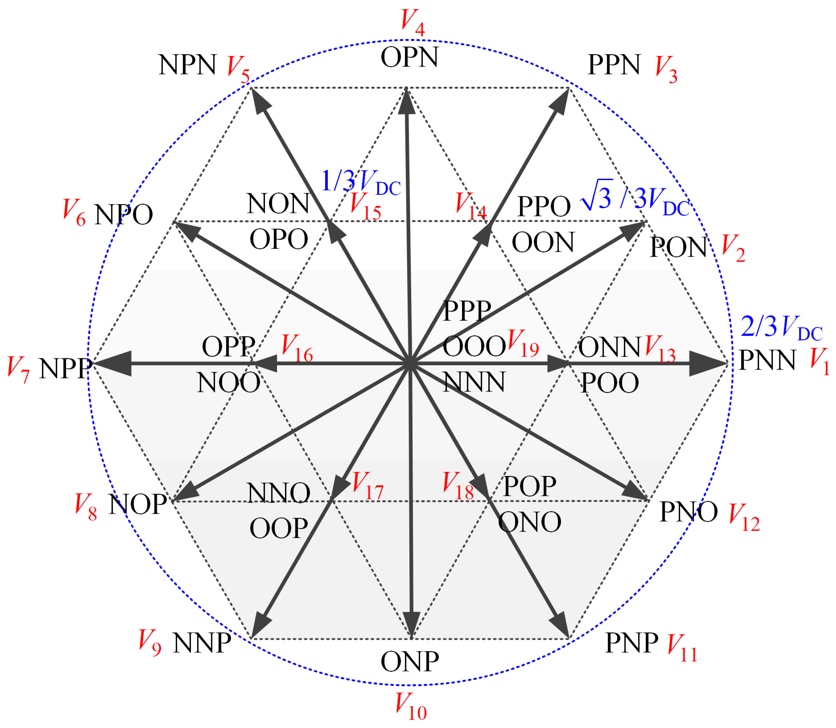
The sector of the voltage vector from the previous control cycle is determined. The 16 voltage vectors from the 2 adjacent regions are selected as the candidate vector set. These candidate vectors are then substituted into Equations (5)–(7) and (10) to obtain T_eN^k+2, ψ_sN^k+2, and v_ON^k+2 at the (k + 2)T_s time step, where N is the voltage vector index.

(4)

Based on Equation (11), the cost function for each candidate voltage vector in the finite control set is calculated. The voltage vector corresponding to the minimum value of the cost function is then selected and applied to the inverter.

4. Improved Predictive Control

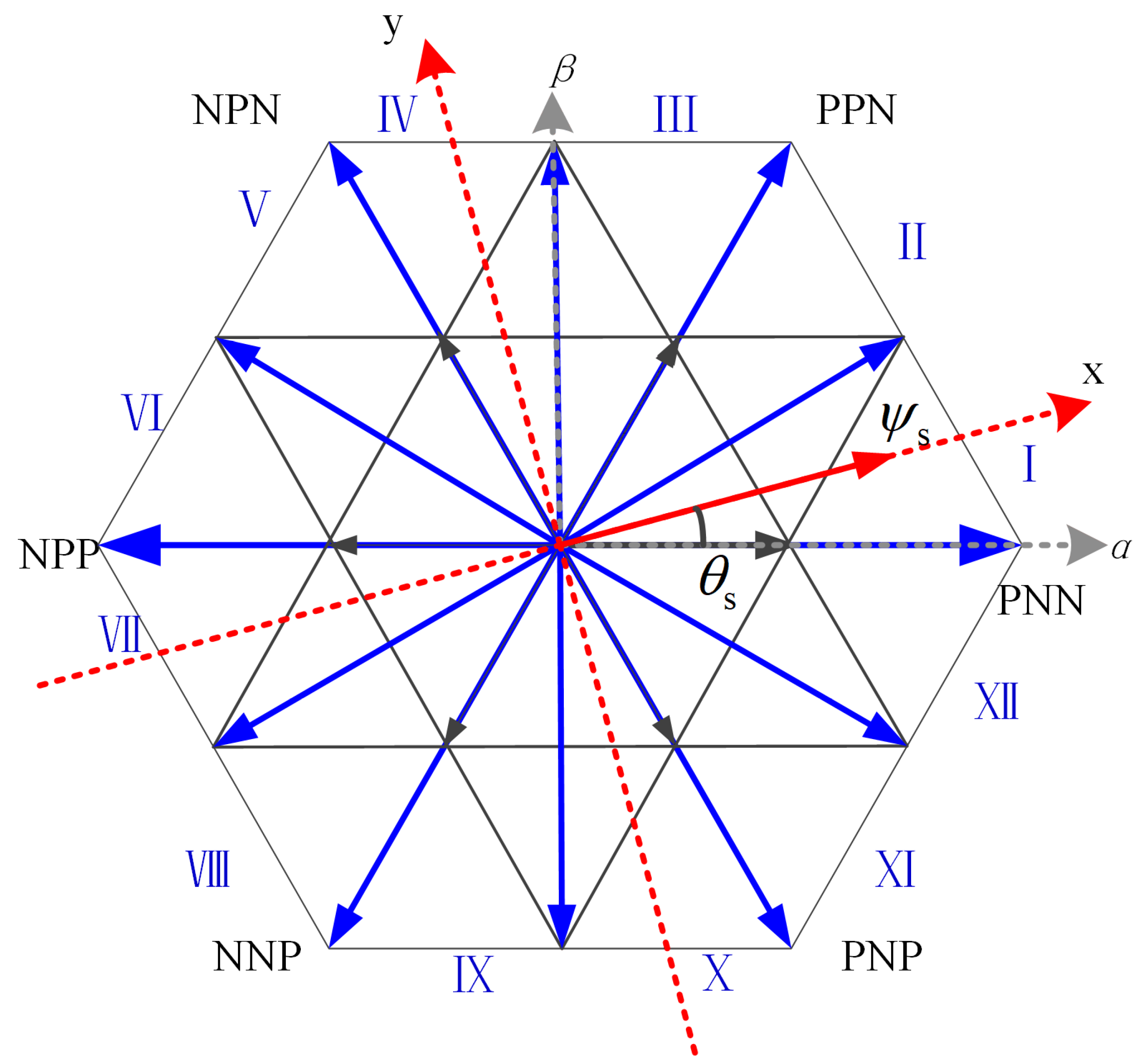
4.1. Vector Sector Selection Strategy

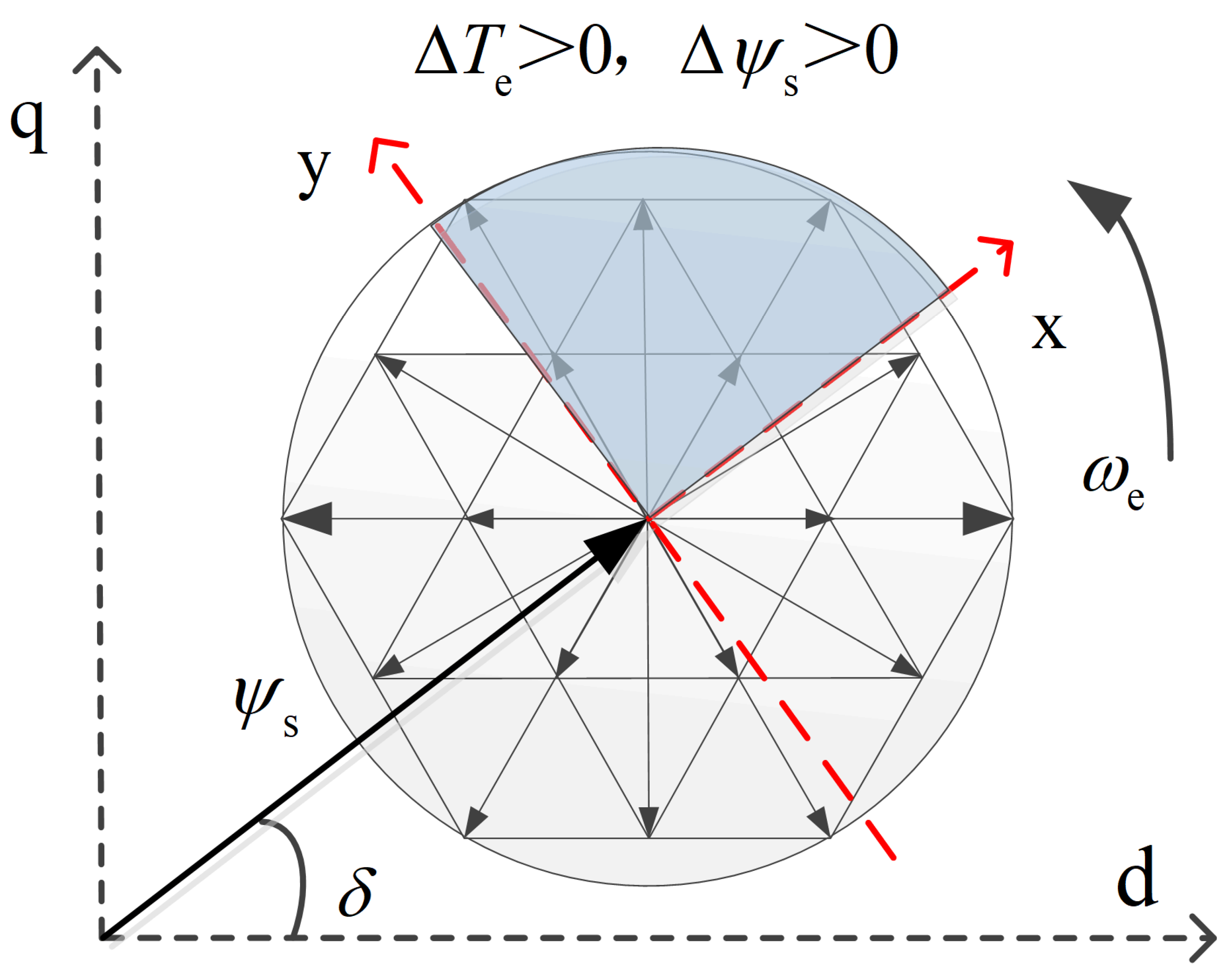
A coordinate system based on the stator flux linkage, referred to as the xy coordinate system, is established. The stator voltage vector equation in the ABC coordinate system is transformed into the xy coordinate system. The transformation relationship is given by the following:

$$\begin{array}{l}{u}_{\mathrm{sx}}=u_{\mathrm{s}}{\mathrm{e}}^{-\mathrm{j}{\theta }_{\mathrm{s}}}\\ i_{\mathrm{sx}}=i_{\mathrm{s}}{\mathrm{e}}^{-\mathrm{j}{\theta }_{\mathrm{s}}}\\ {\psi }_{\mathrm{sx}}={\psi }_{\mathrm{s}}{\mathrm{e}}^{-\mathrm{j}{\theta }_{\mathrm{s}}}\end{array}$$

(12)

$$\begin{array}{l}{\theta }_{\mathrm{s}}={\theta }_{\mathrm{e}}+\delta \\ \delta =\arctan {\displaystyle \frac{{\psi }_{\mathrm{q}}}{{\psi }_{\mathrm{d}}}}\end{array}$$

(13)

where u_s = [u_d, u_q], i_s = [i_d, i_q], and ψ_s = [ψ_d, ψ_q]; θ_e represents the electrical angle of the motor; and δ represents the load angle.

Taking the A-axis as the reference and using π/6 as the interval, the space vector plane is divided into 12 flux linkage sectors in the counterclockwise direction. These sectors are sequentially numbered as Sector I to Sector XII, as shown in Figure 3. The sector where the flux linkage lies is determined by the stator flux linkage angle θ_s. The stator voltage vector equation can be rewritten as follows:

$$\begin{array}{l}{u}_{\mathrm{sx}}=R_{\mathrm{s}}{i}_{\mathrm{sx}}+{\displaystyle \frac{\mathrm{d}{\psi }_{\mathrm{sx}}}{\mathrm{dt}}}\\ u_{\mathrm{sy}}=R_{\mathrm{s}}{i}_{\mathrm{sy}}+{\displaystyle \frac{\mathrm{d}{\psi }_{\mathrm{sy}}}{\mathrm{dt}}}\end{array}$$

(14)

where u_sx and u_sy are the components of the stator voltage in the xy coordinate system, i_sx and i_sy are the components of the stator current in the xy coordinate system, and ψ_sx and ψ_sy are the components of the stator flux linkage in the xy coordinate system.

Neglecting the stator resistance effect and using the motor’s mathematical model with the feedforward Euler method, the stator flux linkage ψ_s^k+1 can be expressed as follows:

$${{\psi }_{\mathrm{s}}}^{k+1}={\psi }_{\mathrm{s}}^k+T_{\mathrm{s}}{u}_{\mathrm{sx}}^k$$

(15)

where ψ_s^k+1 and ψ_s^k represent the stator flux linkage at times k and k + 1, respectively. By differentiating the stator flux linkage and electromagnetic torque with respect to time, the following equation can be obtained:

$$\left\{\begin{array}{c}{\displaystyle \frac{\mathrm{d}{\psi }_{\mathrm{s}}}{\mathrm{d}t}}=u_{\mathrm{sx}}\\ {\displaystyle \frac{\mathrm{d}{T}_{\mathrm{e}}}{\mathrm{d}t}}={\displaystyle \frac{1.5p{\psi }_{\mathrm{s}}{\psi }_{\mathrm{f}}\cos \delta }{L_{\mathrm{s}}}}·{\displaystyle \frac{\mathrm{d}\delta }{\mathrm{d}t}}\end{array}\right.$$

(16)

$$\left\{\begin{array}{l}\Delta {\psi }_{\mathrm{s}}=T_{\mathrm{s}}{u_{\mathrm{sx}}}^k\\ \Delta T_{\mathrm{e}}={\displaystyle \frac{1.5p{\psi }_{\mathrm{f}}\cos \delta }{L_{\mathrm{s}}}}{\psi }_{\mathrm{s}}\left({{\theta }_{\mathrm{s}}}^{k+1}-{{\theta }_{\mathrm{r}}}^{k+1}-{{\theta }_{\mathrm{s}}}^k+{{\theta }_{\mathrm{r}}}^k\right)\end{array}\right.$$

(17)

Within a unit control period T_s, the selected basic voltage vector is applied to the motor, ensuring that the load angle δ remains constant. The following equation can be obtained:

$${{\theta }_{\mathrm{s}}}^{k+1}-{{\theta }_{\mathrm{r}}}^{k+1}-{{\theta }_{\mathrm{s}}}^k+{{\theta }_{\mathrm{r}}}^k=\Delta {\theta }_{\mathrm{s}}$$

(18)

where ∆θ_s denotes the angular variation of the stator flux linkage from time k to time k + 1. The increment of the y-axis component of the stator flux linkage during one control period can be denoted by ∆ψ_sy = ψ_ssin∆θ_s ≈ ψ_s∆θ_s, ψ_s∆θ_s = u_sy. Thus, the variations in the torque and flux linkage, as well as the flux linkage and torque at time k + 1, can be expressed by Equation (19) and a schematic diagram of the torque and flux linkage increments is obtained, as shown in Figure 4.

$$\left\{\begin{array}{l}{\psi }_{\mathrm{s}}^{k+1}={\psi }_{\mathrm{s}}^k+T_{\mathrm{s}}{u_{\mathrm{sx}}}^k\\ T_{\mathrm{e}}^{k+1}=T_{\mathrm{e}}^k+{\displaystyle \frac{1.5p{\psi }_{\mathrm{f}}\cos \delta }{L_{\mathrm{s}}}}{u}_{\mathrm{sy}}\end{array}\right.$$

(19)

Therefore, it can be seen that the variation in torque is determined by u_sx; the variation in flux linkage is determined by u_sy.

From Equation (3), the magnitude of ψ_s^k can be calculated. θ_s determines where the flux linkage sector is located. The computed electromagnetic torque T_e^k+1 and stator flux linkage ψ_s^k+1 are compared with the reference values for electromagnetic torque T_e^ref and stator flux linkage T_e^ref and are, respectively, input into the torque and flux linkage hysteresis loops. The reference torque T_e^ref is obtained from the speed outer loop. The changes in torque and flux linkage can be classified into four cases:

(a)

∆T_e > 0, ∆ψ_s > 0;

(b)

∆T_e > 0, ∆ψ_s < 0;

(c)

∆T_e < 0, ∆ψ_s < 0;

(d)

∆T_e < 0, ∆ψ_s > 0.

After this, the space vector plane is divided into four voltage vector sectors, using the stator flux linkage and its perpendicular direction as boundaries. The sectors are sequentially numbered counterclockwise, starting from the flux linkage position. The voltage vectors within the four sectors sequentially satisfy the above four cases. Figure 5 is a schematic diagram of the candidate voltage vectors contained in ∆T_e > 0, ∆ψ_s > 0.

In this way, the 27 candidate basic voltage vectors are reduced to 8, which are defined as voltage vector set 1. This step reduces the number of candidate voltage vectors and decreases the computational burden.

4.2. Elimination of the Neutral-Point Voltage Weighting Factor

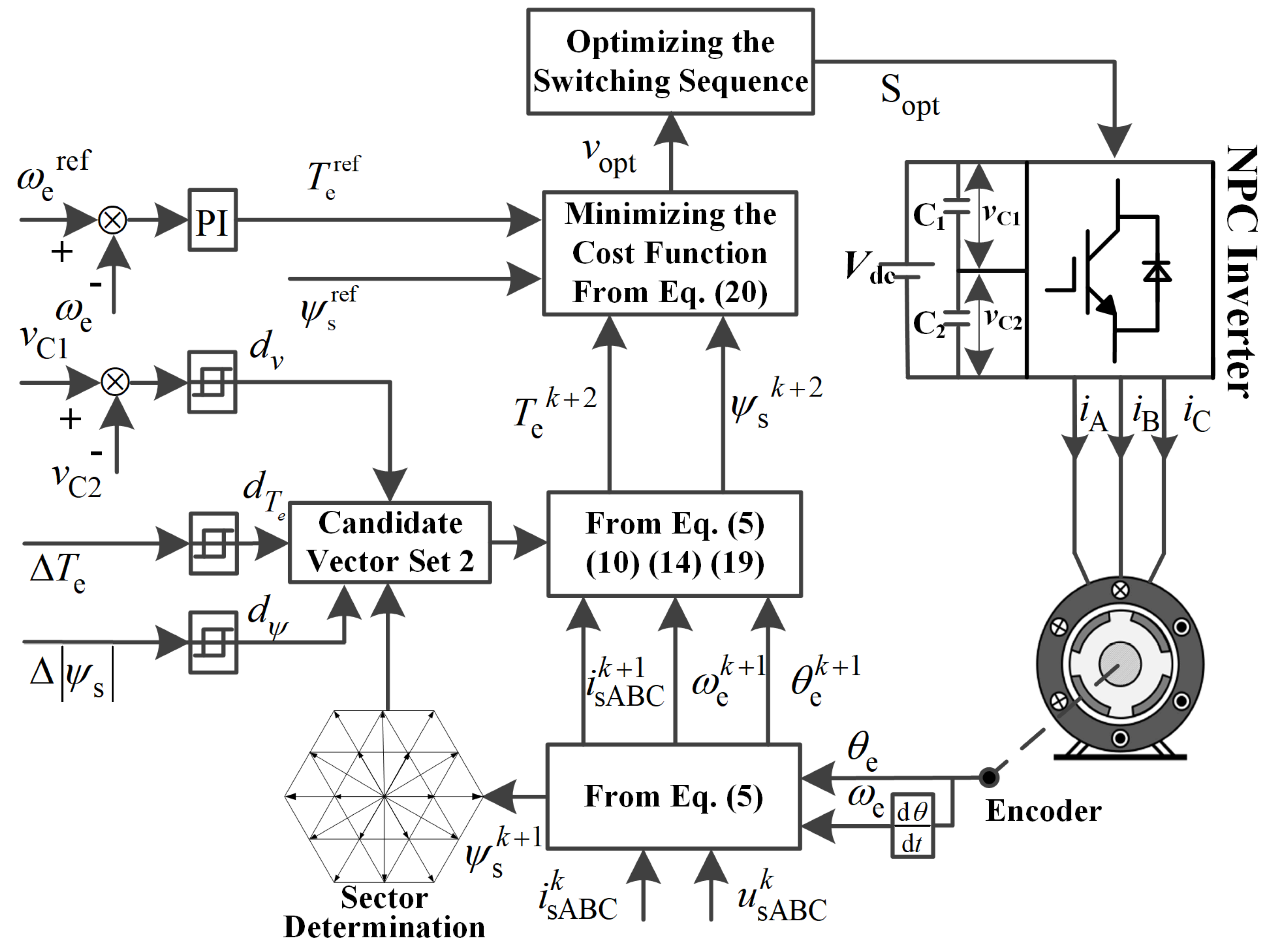
A three-phase AC current generates a rotating stator magnetic field in the motor air gap. The interaction between the stator magnetic field and the permanent magnet field produces electromagnetic torque, driving the rotor’s permanent magnets to rotate. The three-phase stator current exhibits different amplitude relationships in different magnetic field sectors, as shown in

Table 1. Current information contained within the sectors.

Section	iA	iB	iC	Section	iA	iB	iC
I	>0	<0	<0	VII	>0	>0	>0
II	>0	>0	<0	VIII	<0	<0	>0
III	>0	>0	<0	IX	<0	<0	>0
IV	>0	>0	<0	X	>0	<0	>0
V	<0	>0	<0	XI	>0	<0	>0
VI	<0	>0	>0	XII	>0	<0	<0

.

If the inverter sends out a small vector, i_O will flow into or out of the neutral point. For example, for the small vector POO, the corresponding current loop is shown in Figure 6. The neutral-point current i_O is opposite to i_A. If i_A flows in the same direction as the specified positive direction, i.e., toward the load side, the upper capacitor C₁ discharges and the lower capacitor C₂ charges. Conversely, if the direction is reversed, C₁ charges and C₂ discharges. For the other switching state of this small vector, ONN, the neutral-point current is the same as i_A. The effect on the charging and discharging of the capacitors is opposite to the analysis performed during the POO state. Therefore, based on the neutral-point voltage difference and the polarity of the current flowing into the neutral point, the small vectors that cause offset are filtered out using hysteresis. The resulting table can be obtained. As a result, candidate vector set 1 selected in step 5 is reduced from eight vectors to six, further simplifying candidate vector set 1.

The cost function is constructed based on the stator flux linkage, electromagnetic torque, and neutral-point voltage, while optimization is performed to achieve multi-objective optimal control. By further constraining candidate vector set 1 through

Table 2. Small vector redundancy state selection table.

	$\Delta \mathit{u}>0$		$\Delta \mathit{u}<0$
Switching state	$i_{\mathrm{A}}\ge 0$	$i_{\mathrm{A}}<0$	$i_{\mathrm{A}}\ge 0$	$i_{\mathrm{A}}<0$
POO, ONN	ONN	POO	POO	ONN
OPP, NOO	OPP	NOO	NOO	OPP
Switching state	$i_{\mathrm{B}}\ge 0$	$i_{\mathrm{B}}<0$	$i_{\mathrm{B}}\ge 0$	$i_{\mathrm{B}}<0$
OPO, NON	NON	OPO	OPO	NON
POP, ONO	POP	ONO	ONO	POP
Switching state	$i_{\mathrm{C}}\ge 0$	$i_{\mathrm{C}}<0$	$i_{\mathrm{C}}\ge 0$	$i_{\mathrm{C}}<0$
OOP, NNO	NNO	OOP	OPP	NNO
PPO, OON	PPO	OON	OON	PPO

, a new candidate vector set is obtained, which is defined as candidate vector set 2. The small vectors, which can balance the neutral-point voltage, allow the removal of the neutral-point voltage term from the cost function, thus solving the complex issue of tuning the weight coefficients. The cost function can be simplified as follows:

$$g={\lambda }_{\mathsf{\psi }}\left|{\left|{\psi }_s\right|}^{*}-{\left|{\psi }_s\right|}^{k+2}\right|+{\lambda }_{\mathrm{T}}\left|T_{\mathrm{e}}^{*}-T_{\mathrm{e}}^{k+2}\right|$$

(20)

At this point, only the stator flux linkage and electromagnetic torque need to be optimized to achieve optimal control for these two objectives. Fast predictive torque control is implemented, the minimum value of the cost function is calculated, and the basic voltage vector corresponding to this minimum value is the optimal voltage vector.

The weighting coefficient λ_T for the torque is set to 1, and the weighting coefficient λ_ψ for the flux linkage is set to 230. The weighting coefficients for the torque and flux linkage are selected through repeated simulations and experiments to achieve better control performance. This results in the control block diagram shown in Figure 7.

The proposed model predictive control process is as follows:

(1)

Information about the three-phase currents i_A, i_B, i_C, ω_e, and θ_e and the neutral-point voltage v_O of the PMSM at time (k)T_s is obtained.

(2)

Sampling and calculation delay compensation are performed. The data collected in the first step are used, and Equation (5) is applied to obtain i_d^k+1 and i_q^k+1 at time (k + 1)T_s, which are then used as the initial values for the next prediction step.

(3)

The electrical angular speed and its reference value are input into the speed outer loop, which results in the reference torque T_e^ref. The voltage difference between the upper and lower capacitors is input into the neutral-point voltage hysteresis comparator, resulting in ∆v_O. The predicted torque value T_e^k+1 and the reference torque value T_e^ref are input into the torque hysteresis comparator, resulting in ∆T_e. The predicted flux linkage value ψ_s^k+1 and the reference flux linkage value ψ_s ^ref are input into the flux linkage hysteresis comparator to determine the torque–flux linkage hysteresis, resulting in ∆|ψ_s|.

(4)

The values ∆v_O, ∆T_e, and ∆|ψ_s| from the previous steps are input into the candidate voltage vector selection mechanism, resulting in candidate voltage vector set 2. Each candidate voltage vector set 2 contains six basic voltage vectors. By substituting the six basic voltage vectors, along with i_d^k+1, i_q^k+1, w_e^k+1, and θ_e^k+1, into Equations (5), (14), (19), and (10), T_eN^k+2, T_eN^k+2, ψ_sN^k+2, and v_ON^k+2 at time (k + 2)T_s are obtained, where N represents the voltage vector index.

(5)

Based on Equation (20), the cost function corresponding to each candidate voltage vector in candidate vector set 2 is calculated. The voltage vector corresponding to the minimum value of the cost function is selected and applied to the inverter.

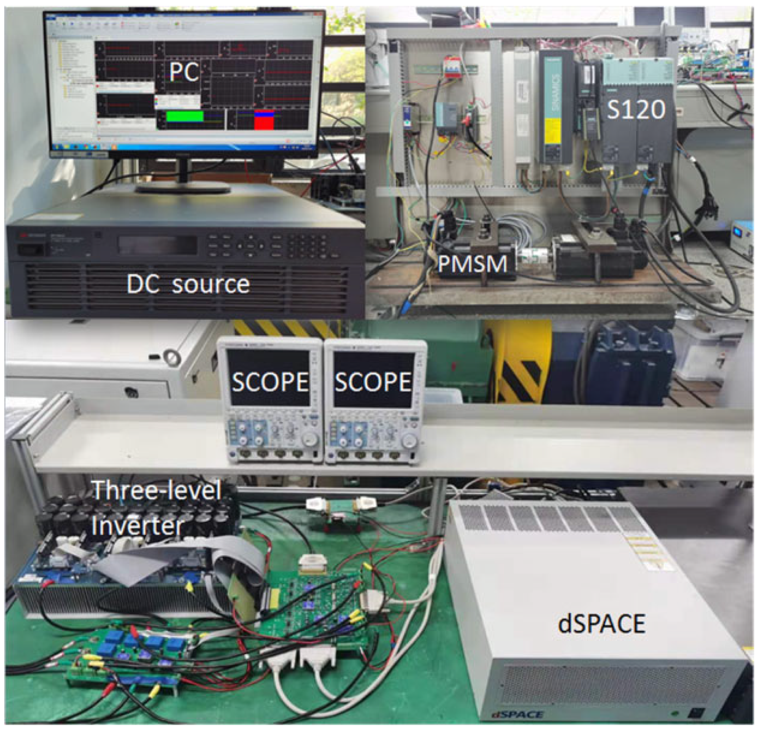
5. Experimental Analysis and Validation

To verify the feasibility and effectiveness of the proposed improved MPTC algorithm, an experimental system powered by an NPC three-level inverter and a PMSM is built, as shown in Figure 8. In this system, the dSPACE^® DS1007 rapid development model (Shanghai, China) is used as the controller, and the SIEMENS^® S120 (Beijing, China) is used as the inverter driven dynamometer. The parameters of the PMSM are shown in

Table 3. Motor parameters.

Parameters	Symbol	Value	Unit
Number of poles	p	2	poles
Permanent magnet flux linkage	ψf	0.45	Wb
Stator resistance	Rs	0.635	Ω
d/q-axis inductance	Ld/Lq	4.25	mH
Rated speed	nr	1500	r/min
Rated torque	TN	10	N·m
Rated voltage	VN	220	V
Sampling frequency	Ts	10	kHz

, where the proportional gain of the speed loop PI controller is 0.2 and the integral gain is 6.7.

The experimental phenomena of the three model predictive control methods are analyzed and compared. The traditional model predictive control is referred to as MPTC1. The control method, with a neutral point voltage term in the cost function, is referred to as MPTC2. The control method that removes the neutral point voltage term from the cost function by employing neutral point voltage hysteresis is referred to as MPTC3.

5.1. Comparative Analysis of the Steady-State Performance

When the motor operates at a speed of n_r = 500 r/min and a load of 10 Nm, the upper and lower capacitor voltages U_po and U_no, electrical angular speed w_e, electromagnetic torque T_e, and the stator current waveform of phase i_A are as shown in Figure 9. Figure 9a shows the waveforms under MPTC1 (λ_T = 1, λ_ψ = 230, λ_v = 0.01). Figure 9b shows the waveforms under MPTC2 (λ_T = 1, λ_ψ = 230, λ_v = 0.01). Figure 9c shows the waveforms under MPTC3 (λ_T = 1, λ_ψ = 230, λ_v = 0.01). The torque hysteresis width T_e_bw is set to 0.01 T_n, the flux linkage hysteresis width ψ_bw is set to 0.015ψ_f, and the neutral point voltage hysteresis width V_O_bw is set to 1 V.

When the motor operates under low speed and low load conditions, as shown in Figure 9, it can be observed that MPTC2, compared to MPTC1, reduces the number of candidate vectors, and the stator current waveform is optimized. As shown in

Table 4. Comparison of the output performance of the three strategies.

Strategy	nr (r/min)	TL (N·m)	ITHD	Uripple (V)
MPTC1	500	10	27.40%	7.1
MPTC1	1500	15	32.53%	6.5
MPTC2	500	10	21.79%	6.1
MPTC2	1500	15	16.15%	5.5
MPTC3	500	10	20.63%	6.6
MPTC3	1500	15	16.67%	6.6

, under the condition of motor speed n_r = 500 r/min and load torque T_L = 10 N·m, the THD of the current waveform under MPTC1~3 strategies are 27.40%, 21.79%, and 20.63%, respectively. Under the condition of motor speed n_r = 1500 r/min and load torque T_L = 15 N·m, the THD of the current waveform under MPTC1~3 strategies are 32.53%, 16.15%, and 16.07%, respectively. The strategy proposed in this paper reduces the output current THD under different operating conditions. Where U_ripple is the difference between the upper and lower capacitor voltages, the setting of the torque hysteresis width suppresses torque fluctuations, and the neutral point voltage also tends to balance. MPTC3, compared to MPTC2, removes the neutral point voltage term from the cost function, leaving only the torque and flux linkage terms. Therefore, it better satisfies the requirements for torque and speed. It can be seen that torque fluctuations and speed fluctuations are smaller, and the neutral-point voltage is balanced through neutral point voltage hysteresis.

The above experimental phenomena indicate that, while enhancing the system’s dynamic performance, the stability of the system can also be maintained.

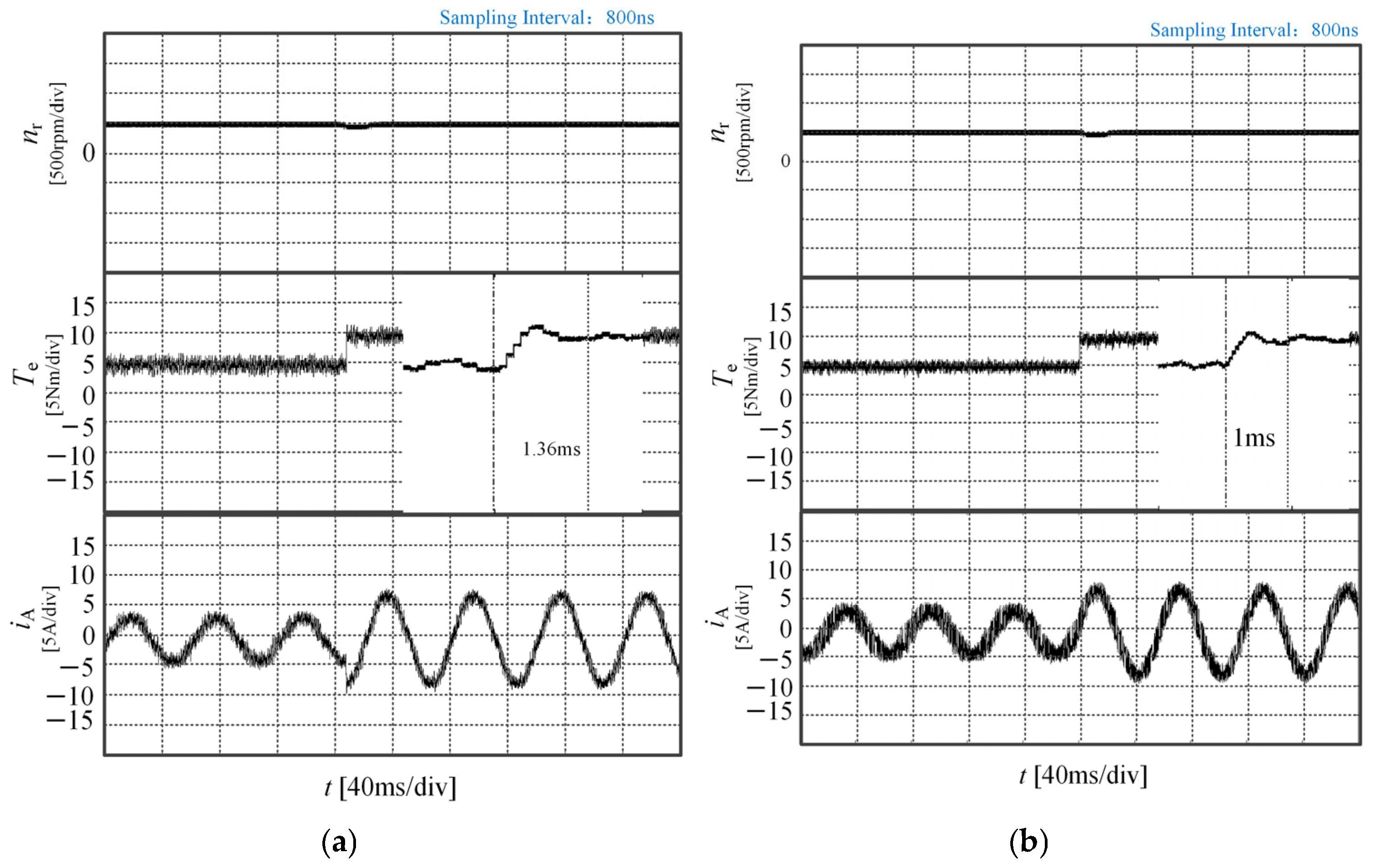
5.2. Comparative Analysis of Dynamic Performance

To test the system’s fast dynamic response performance, a sudden load is applied at a specific time, and its dynamic tracking performance is observed.

When the motor operates at 500 r/min and the torque is 5 Nm, a sudden load is applied to increase the torque to 10 Nm. Figure 10a,b shows the waveforms of the electrical angular speed w_e, electromagnetic torque T_e, and stator current i_A of phase A under the MPTC1 and MPTC3 control methods, respectively. It can be observed that with the MPTC1 control method, the time required for the torque to change from 5 Nm to 10 Nm is 1.36 ms, while with the MPTC3 control method, it only takes 1 ms. The current transition is also more continuous and approaches a sine wave. The reduction in the number of candidate vectors clearly demonstrates better dynamic performance, and the speed can be well maintained at 500 r/min.

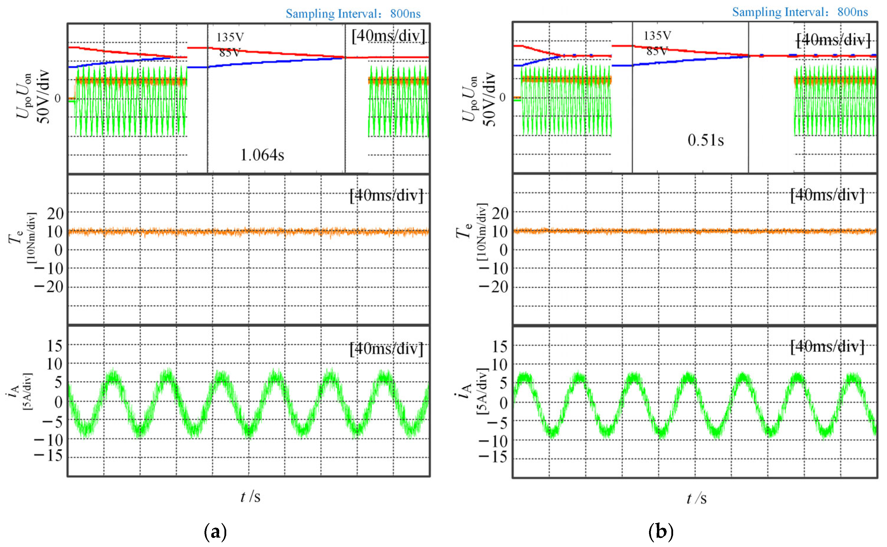
5.3. Neutral-Point Voltage Balancing Capability

When the upper and lower capacitor voltages become unbalanced, they can be balanced by the MPTC3 control algorithm, ensuring that the neutral-point voltage remains stable. In Figure 11, the DC bus U_DC is 220 V, with the upper capacitor voltage at 135 V and the lower capacitor voltage at 85 V. The difference between the upper and lower capacitor voltages is 50 V. The motor operates at a speed of n_r = 500 r/min under a load of 10 Nm. Figure 11a shows the neutral-point voltage balancing capability under the MPTC2 control algorithm. The time required to restore balance from the unbalanced state is 1.064 s. Figure 11b displays the MPTC3 control algorithm. The time needed to restore balance is 0.51 s. As shown in

Table 5. The capacitor recovery balance time under different operating conditions.

Strategy	nr (r/min)	TL (N·m)	tbalance (s)
MPTC2	500	10	1.064
MPTC2	1000	5	4.62
MPTC3	500	10	0.51
MPTC3	1000	5	4.61

, at n_r = 500 r/min and T_L = 10 N·m, the capacitor voltage recovery time for MPTC3 is reduced by 52% compared to MPTC2. At n_r = 1000 r/min and T_L = 5 N·m, the capacitor voltage recovery times are almost the same. In MPTC2, capacitor balancing is achieved through the cost function, whereas in MPTC3, it is achieved through the hysteresis control loop. The capacitor voltage balance is a term in the cost function, and its balancing capability is related to its weight coefficient. As the capacitor voltage approaches balance, this term’s contribution to the cost function decreases, affecting its ability to balance the midpoint voltage. MPTC3 uses the hysteresis control loop to balance the midpoint voltage, effectively suppressing midpoint voltage fluctuations in any given cycle, resulting in a stronger balancing capability than MPTC2. However, compared to low modulation cases (n_r = 500 r/min), in high modulation cases (n_r = 1000 r/min), the longer duration of large vector actions, which do not produce a midpoint current, leads to similar capacitor voltage recovery times for both strategies. In either of these cases, the motor output torque is always stabilized.

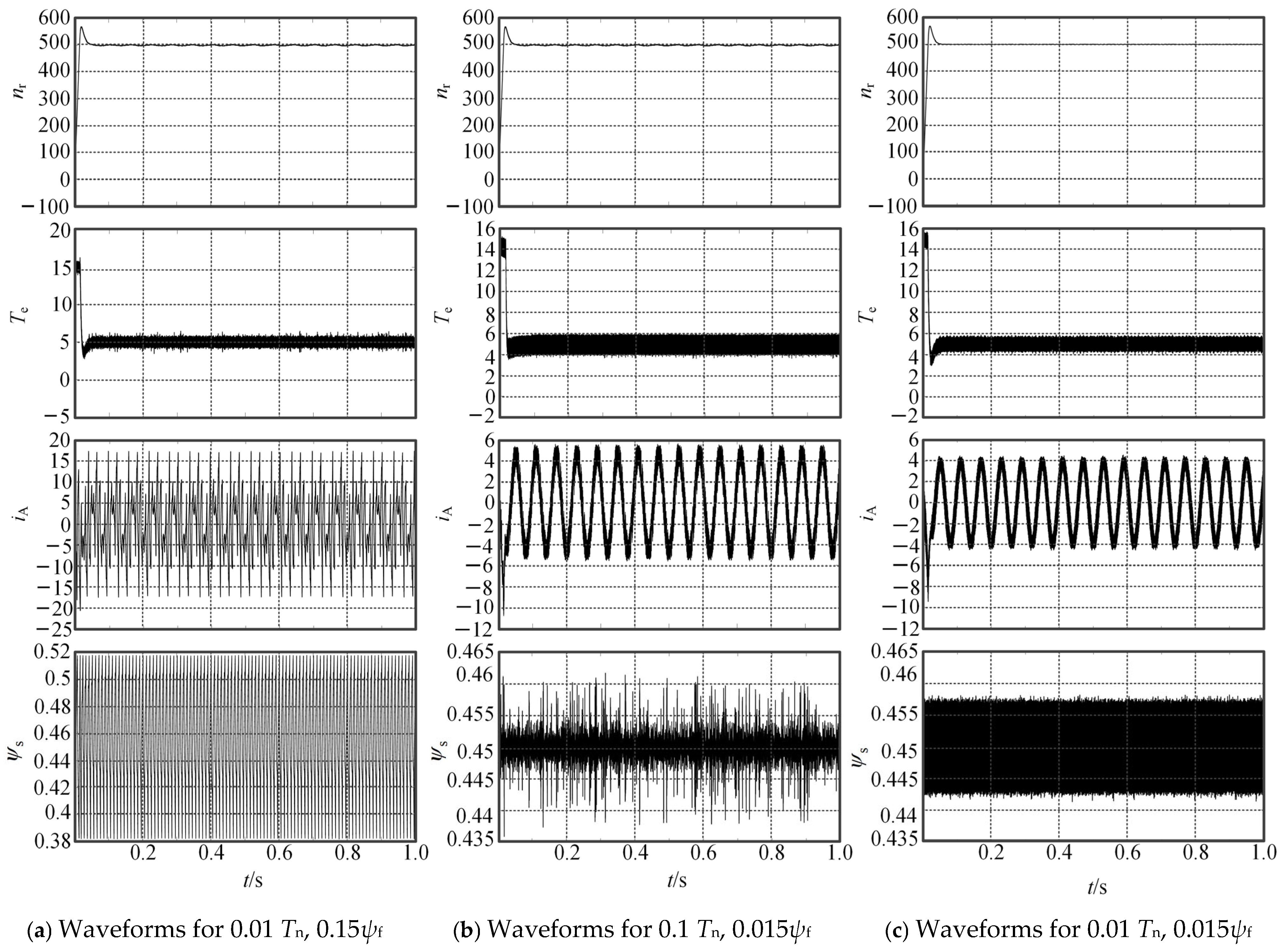
5.4. The Sensitivity Analysis of Hysteresis Thresholds

A simulation was added to better explain the strategy presented in this paper. Figure 12 shows the effect of different hysteresis widths on the system’s speed, torque, phase A current, and flux linkage under the conditions of n_r = 500 r/min and T_L = 5 Nm. Figure 12a–c represents the cases where the torque hysteresis width and flux linkage hysteresis width are set to 0.01 T_n and 0.15ψ_f, 0.1 T_n and 0.015ψ_f, and 0.01 T_n and 0.015ψ_f, respectively, where T_n is the rated torque of the motor and ψ_f is the flux linkage of the motor’s permanent magnet.

With a torque hysteresis of 0.01 T_n, torque tracking is smooth with minor fluctuations (~2 N·m), but current waveforms show large spikes. Increasing it to 0.1 T_n improves the current quality but worsens torque tracking. When flux hysteresis is 0.15ψ_f, the flux and speed fluctuate noticeably, whereas 0.015ψ_f enables accurate flux tracking. These results show that hysteresis widths significantly affect the control objectives and system stability. Therefore, 0.01 T_n and 0.015ψ_f are chosen for the improved model predictive torque control to ensure optimal performance.

6. Conclusions

A three-level MPTC finite-set predictive method and a neutral point voltage balancing strategy are investigated in this paper. A new three-level finite-set predictive control method, considering neutral point voltage balancing for PMSM, is proposed. The mathematical model of the PMSM is first analyzed. Then, the motor torque, flux linkage, and neutral point voltage are each predicted using the predictive model, and a cost function is constructed. Furthermore, the flux linkage position and the flux linkage hysteresis output state are used to effectively select vectors. By introducing neutral point voltage hysteresis, redundant small vectors with neutral point voltage balancing capability are selected. Thus, the need for additional neutral point voltage weighting coefficient tuning is avoided, and neutral point voltage fluctuations are effectively suppressed.

References

1. Choi, H.H.; Vu, T.T.; Jung, J.W. Digital Implementation of an Adaptive Speed Regulator for a PMSM. IEEE Trans. Power Electron. 2011, 26, 3–8. [Google Scholar] [CrossRef]
2. Liu, H.; Zhu, Z.Q.; Mohamed, E.; Fu, Y.; Qi, X. Flux-Weakening Control of Nonsalient Pole PMSM Having Large Winding Inductance, Accounting for Resistive Voltage Drop and Inverter Nonlinearities. IEEE Trans. Power Electron. 2012, 27, 942–952. [Google Scholar] [CrossRef]
3. Cho, Y.; Lee, K.; Song, J.; Lee, Y.I. Torque-ripple minimization and fast dynamic scheme for torque predictive control of permanent-magnet synchronous motors. IEEE Trans. Power Electron. 2015, 30, 2182–2190. [Google Scholar] [CrossRef]
4. Mourabit, Y.E.; Derouich, A.; Abdelaziz, E.G.; Ouanjli, N.E.; Othmane, Z. Dtc-svm control for permanent magnet synchronous generator based variable speed wind turbine. Int. J. Power Electron. Drive Syst. 2017, 8, 1732–17432. [Google Scholar] [CrossRef]
5. Mukherjee, S.; Giri, S.K.; Banerjee, S. A Flexible Discontinuous Modulation Scheme With Hybrid Capacitor Voltage Balancing Strategy for Three-Level NPC Traction Inverter. IEEE Trans. Ind. Electron. 2019, 66, 3333–3343. [Google Scholar]
6. Mohammed, E.M.; Badre, B.; Najib, E.O.; Abdelilah, H.; Houda, E.A.; Btissam, M.; Said, M. Predictive Torque and Direct Torque Controls for Doubly Fed Induction Motor: A Comparative Study. In Proceedings of the International Conference on Digital Technologies and Applications, Fez, Morocco, 28 January 2022. [Google Scholar]
7. El Daoudi, S.; Lazrak, L.; El Ouanjli, N. New Contributions for Speed Observation of Asynchronous Motor Fed by Multilevel Inverter. Aust. J. Electr. Electron. Eng. 2023, 20, 279–290. [Google Scholar]
8. Choundhury, A.; Pillay, P.; Williamson, S.S. Comparative analysis between two-level and three-level DC/AC electric vehicle traction inverters using a novel DC-link voltage balancing algorithm. IEEE J. Emerg. Sel. Top. Power Electron. 2014, 2, 529–540. [Google Scholar]
9. Teichmann, R.; Bernet, S. A comparison of three-level converters versus two-level converters for low-voltage drives traction and utility applications. IEEE Trans. Ind. Appl. 2005, 41, 855–865. [Google Scholar]
10. Schweizer, M.; Friedli, T.; Kolar, J.W. Comparative evaluation of advanced three-phase three-level inverter/converter topologies against two-level systems. IEEE Trans. Ind. Electron. 2013, 60, 5515–5527. [Google Scholar] [CrossRef]
11. Zhang, X.; Hou, B. Double Vectors Model Predictive Torque Control Without Weighting Factor Based on Voltage Tracking Error. IEEE Trans. Power Electron. 2018, 33, 2368–2380. [Google Scholar] [CrossRef]
12. Mohan, D.; Zhang, X.; Foo, G.H.B. A Simple Duty Cycle Control Strategy to Reduce Torque Ripples and Improve Low-Speed Performance of a Three-Level Inverter Fed DTC IPMSM Drive. IEEE Trans. Ind. Electron. 2017, 64, 2709–2721. [Google Scholar] [CrossRef]
13. Fuentes, E.; Cesar, A.; Silva Kennel, R.M. MPC Implementation of a Quasi-Time-Optimal Speed Control for a PMSM Drive, With Inner Modulated-FS-MPC Torque Control. IEEE Trans. Ind. Electron. 2016, 63, 3897–3905. [Google Scholar] [CrossRef]
14. Kakosimos, P.; Abu-Rub, H. Deadbeat Predictive Control for PMSM Drives With 3-L NPC Inverter Accounting for Saturation Effects. IEEE J. Emerg. Sel. Top. Power Electron. 2018, 6, 1671–1680. [Google Scholar] [CrossRef]
15. Wang, Q.; Yu, H.; Li, C.; Lang, X. A Low-Complexity Optimal Switching Time-Modulated Model-Predictive Control for PMSM With Three-Level NPC Converter. IEEE Trans. Transp. Electrif. 2020, 6, 1188–1198. [Google Scholar] [CrossRef]
16. Garcia, G.A.; Keshmiri, S.S.; Stastny, T. Robust and Adaptive Nonlinear Model Predictive Controller for Unsteady and Highly Nonlinear Unmanned Aircraft. IEEE Trans. Control Syst. Technol. 2015, 23, 1620–1627. [Google Scholar] [CrossRef]
17. Gao, J.; Gong, C.; Li, W.; Liu, J. Novel Compensation Strategy for Calculation Delay of Finite Control Set Model Predictive Current Control in PMSM. IEEE Trans. Ind. Electron. 2020, 67, 5816–5819. [Google Scholar] [CrossRef]
18. Geyer, T. Computationally efficient model predictive direct torque control. IEEE Trans. Power Electron. 2011, 26, 2804–2816. [Google Scholar] [CrossRef]
19. Geyer, T.; Quevedo, D.E. Quevedo Multistep finite control set model predictive control for power electronics. IEEE Trans. Power Electron. 2014, 29, 6836–6846. [Google Scholar] [CrossRef]
20. Wang, F.; Zhang, Z.; Kennel, R.; Rodriguez, J. Model predictive torque control with an extended prediction horizon for electrical drive systems. Int. J. Control 2015, 88, 1379–1388. [Google Scholar] [CrossRef]
21. Habibullah, M.; Lu, D.C.; Rahman, M.F. A simplified finite-state predictive direct torque control for induction motor drive. IEEE Trans. Ind. Electron. 2016, 63, 3964–3975. [Google Scholar] [CrossRef]
22. Xia, C.; Liu, T.; Song, Z. A simplified finite-control-set model-predictive control for power converters. IEEE Trans. Ind. Inform. 2014, 10, 991–1002. [Google Scholar]
23. Cortes, P.; Wilson, A.; Kouro, S. Model predictive control of multilevel cascaded h-bridge inverters. IEEE Trans. Ind. Electron. 2010, 57, 2691–2699. [Google Scholar] [CrossRef]
24. Iqbal, A.; Abu-Rub, H.; Ahmed, S.K.M. Model predictive current control of a three-level five-phase NPC VSI using simplified computational approach. In Proceedings of the 2014 IEEE Applied Power Electronics Conference and Exposition (APEC), Fort Worth, TX, USA, 16–20 March 2014. [Google Scholar]
25. Zhang, Y.; Xie, W.; Li, Z.; Zhang, Y. Low-complexity model predictive power control: Double-vector-based approach. IEEE Trans. Ind. Electron. 2014, 61, 5871–5880. [Google Scholar] [CrossRef]
26. Hu, J.; Zhu, J.; Lei, G.; Platt, G.; Dorrell, D.G. Multi-objective model-predictive control for high-power converters. IEEE Trans. Energy Convers. 2013, 28, 652–663. [Google Scholar]
27. Vyncke, T.J.; Thielemans, S.; Melkebeek, J.A. Finite-set model-based predictive control for flying-capacitor converters: Cost function design and efficient FPGA implementation. IEEE Trans. Ind. Inform. 2013, 9, 1113–1121. [Google Scholar] [CrossRef]
28. Zhang, Z.; Kennel, R. Novel ripple reduced direct model predictive control of three-level NPC active front end with reduced computational effort. In Proceedings of the 2015 IEEE International Symposium on Predictive Control of Electrical Drives and Power Electronics(precede), Valparaiso, Chile, 5–6 October 2015. [Google Scholar]
29. Peng, S.; Zhang, G.; Zhou, Z.; Gu, X.; Xia, C. MPTC of NP-clamped three-level inverter-fed permanent-magnet synchronous motor system for NP potential imbalance suppression. IET Electr. Power Appl. 2020, 14, 658–667. [Google Scholar] [CrossRef]
30. Mora, A.; Donoso, F.; Urrutia, M.; Angulo, A.; Cárdenas, R. Predictive Control Strategy for an Induction Machine fed by a 3L-NPC Converter with Fixed Switching Frequency and Improved Tracking Error. In Proceedings of the 2018 IEEE 27th International Symposium on Industrial Electronics (ISIE), Cairns, QLD, Australia, 13–15 June 2018. [Google Scholar]
31. Khalilzadeh, M.; Vaez-Zadeh, S. Computation Efficiency and Robustness Improvement of Predictive Control for PMS Motors. IEEE J. Emerg. Sel. Top. Power Electron. 2020, 8, 2645–2654. [Google Scholar] [CrossRef]
32. Lewicki, A.; Krzeminski, Z.; Abu-Rub, H. Space-vector pulse-width modulation for three-level NPC converter with the neutral point voltage control. IEEE Trans. Ind. Electron. 2011, 58, 5076–5086. [Google Scholar] [CrossRef]
33. Li, C.; Yang, T.; Kulsangcharoen, P.; Calzo, G.L.; Bozhko, S.; Gerada, C. A Modified Neutral Point Balancing Space Vector Modulation for Three-Level Neutral Point Clamped Converters in High-Speed Drives. IEEE Trans. Ind. Electron. 2019, 66, 910–921. [Google Scholar] [CrossRef]
Figure 1. NPC three-level inverter topology.
Wevj 16 00254 g001
Figure 2. Spatial vector diagram.
Wevj 16 00254 g002
Figure 3. Schematic diagram of flux linkage sector division.
Wevj 16 00254 g003
Figure 4. Schematic diagram of the torque and flux linkage increments.
Wevj 16 00254 g004
Figure 5. Schematic diagram of voltage vector selection.
Wevj 16 00254 g005
Figure 6. Small vector POO-state diagram.
Wevj 16 00254 g006
Figure 7. System control block diagram.
Wevj 16 00254 g007
Figure 8. Physical diagram of the system.
Wevj 16 00254 g008
Figure 9. Waveforms under steady-state conditions. (a) MPTC1, (b) MPTC2, (c) MPTC3. (The sampling interval (800 ns) refers to the oscilloscope’s sampling interval).
Wevj 16 00254 g009
Figure 10. Dynamic performance. (a) MPTC1, (b) MPTC3.
Wevj 16 00254 g010
Figure 11. Neutral point voltage balancing capability. (a) MPTC2, (b) MPTC3.
Wevj 16 00254 g011
Figure 12. Simulation waveforms for different hysteresis widths.
Wevj 16 00254 g012