Design and Analysis of an MPC-PID-Based Double-Loop Trajectory Tracking Algorithm for Intelligent Sweeping Vehicles

Abstract

To enhance the precision and real-time performance of trajectory tracking control in differential-steering intelligent sweeping robots and to improve the adaptability of the control algorithm to errors caused by sensor noise, tire slip, and skid, an MPC-PID (Model Predictive Control–Proportional-Integral-Derivative) dual closed-loop control strategy was proposed. This strategy integrates a Kalman filter-based state estimator and a sliding compensation module. Based on the kinematic model of the intelligent sweeping robot, a model predictive controller (MPC) was designed to regulate the vehicle’s pose, while a PID controller was used to adjust the longitudinal speed, forming a dual closed-loop control algorithm. A Kalman filter was employed for state estimation, and a sliding compensation module was introduced to mitigate wheel slip and lateral drift, thereby improving the stability of the control system. Simulation results demonstrated that, compared to traditional MPC control, the maximum lateral deviation, maximum heading angle deviation, and speed response time were reduced by 50.83%, 53.65%, and 7.10%, respectively, during sweeping operations. In normal driving conditions, these parameters were improved by 41.58%, 45.54%, and 24.17%, respectively. Experimental validation on an intelligent sweeper platform demonstrates that the proposed algorithm achieves a 16.48% reduction in maximum lateral deviation and 9.52% faster speed response time compared to traditional MPC, effectively validating its enhanced tracking effectiveness in intelligent cleaning operations.

1. Introduction

Intelligent robotic vehicles have been widely applied in the agricultural [1], industrial [2,3], and urban environmental cleaning sectors. Particularly, intelligent cleaning vehicles deployed in campuses, factories, and public spaces can significantly improve operational efficiency and reduce labor costs through autonomous path planning and task execution [4]. As a core technology for enabling intelligent operations, trajectory tracking control [5] is often affected by multiple factors in terms of precision and response speed. During turning maneuvers, wheel–ground relative sliding occurs due to the difference in path lengths between inner and outer wheels, leading to vehicle slippage and wheel spin. These phenomena significantly increase trajectory tracking deviations [6]. Additionally, during vehicle operation, sensor systems are susceptible to environmental interference and inherent errors arising from data transmission processes, which degrade the system’s control accuracy. Therefore, it is imperative to develop trajectory tracking control strategies with fast response speed and high precision to address these challenges.

In the field of trajectory tracking, scholars and experts worldwide have developed various controllers, such as fuzzy control [7], sliding mode control [8], PID control [9], Model Predictive Control (MPC) [10], and Linear Quadratic Regulator (LQR) control [11]. Wang et al. [12] proposed a backstepping control algorithm based on a planar disturbance observer to solve the problem of achieving longitudinal, lateral, and yaw joint trajectory tracking of autonomous driving vehicles under conditions of nonlinear coupling and motion disturbance, thereby avoiding the modeling errors introduced by linearization. Wang et al. [13] proposed a Flatness Model Predictive Control (FMPC) algorithm that uses the flatness condition of the controlled object to accurately convert the original nonlinear system into the Brunovsky standard form, thereby avoiding the modeling error caused by continuous linearization and reducing the computational burden of real-time MPC. Differential flatness provides a rigorous theoretical basis and helps to decompose complex nonlinear dynamic systems into simpler and more decoupled subsystems. Yuan et al. [14] proposed a robust controller with adaptive slip disturbance compensation based on differential flatness. Differential flatness provides a rigorous theoretical foundation that helps decompose complex nonlinear dynamic systems into simpler, more decoupled subsystems. Tang et al. [15] proposed a Robust Model Predictive Control (RMPC) strategy by constructing a min-max formulation robustness optimization function, which enhances both tracking accuracy and adaptability. Meng et al. [16] proposed a hybrid prediction strategy combining short- and long-horizon models, significantly improving path-tracking performance while balancing control accuracy and computational efficiency. Viana et al. [17] developed a nonlinear MPC approach incorporating longitudinal velocity auxiliary constraints using mixed-integer quadratic programming, achieving enhanced tracking precision. Their experimental validation demonstrated high effectiveness in formation positioning, trajectory tracking, and obstacle avoidance in complex environments. Additionally, Li et al. [18] proposed a nonlinear MPC method to improve longitudinal and lateral stability under extreme driving conditions. Numerous researchers have dedicated efforts to exploring trajectory tracking control methods for intelligent cleaning vehicles, with a focus on addressing challenges such as environmental disturbances and multi-speed adaptability. Yao et al. [19] addressed the unknown parameter control problem in unmanned intelligent cleaning vehicle systems by reformulating the trajectory tracking control as a pre-aiming deviation angle tracking control issue. They proposed an improved Model-Free Adaptive Control (MFAC)-based trajectory tracking scheme to enhance robustness under parameter uncertainties. Li et al. [20] designed a hybrid controller that switches between sliding mode control (SMC) at low speeds and model predictive control (MPC) at high speeds. This approach significantly improved the tracking accuracy of intelligent cleaning vehicles across varying operational speeds. Jeong et al. [21] developed an MPC-based trajectory tracking algorithm with rollover prevention for intelligent cleaning vehicles. By optimizing articulated angles and velocities based on a kinematic model, their method not only enhanced tracking precision but also ensured safety against lateral instability.

Traditional control methods, such as fuzzy control and sliding mode control (SMC), may suffer from insufficient precision, high computational complexity, and response delays when handling external disturbances and system uncertainties. In contrast, Model Predictive Control (MPC) effectively addresses multivariable coupling in systems and explicitly incorporates constraints during optimization, thereby enhancing its adaptability in complex environments. However, MPC requires significant computational resources, which limits its real-time performance. In highly dynamic scenarios, this may lead to response lag. To mitigate the high computational complexity and real-time limitations of MPC, PID control leverages its rapid dynamic response capability to correct small-scale errors within short timeframes, thereby improving system stability. Achieving high-precision tracking and fast response speed under limited computational resources.

Current research has rarely considered the combined effects of inherent slip-skid dynamics, sensor measurement errors, and response hysteresis during the trajectory tracking of intelligent cleaning vehicles. To address these limitations, this paper proposes a dual-loop trajectory tracking control strategy integrating a Kalman state estimator and slip compensation, which combines Model Predictive Control and PID control. In this method, the outer loop employs Model Predictive Control (MPC) to achieve real-time prediction and optimization of the vehicle’s pose, ensuring smooth control commands under multivariable and nonlinear constraints. The inner loop uses a PID controller to precisely regulate vehicle speed, enabling a rapid response to dynamic changes in vehicle dynamics. Simultaneously, a sliding compensation mechanism is adopted to mitigate errors caused by tire sideslip, and a Kalman filter with a forgetting factor is introduced to enhance the robustness of state estimation. Compared with existing approaches that primarily rely on a single control strategy (such as pure MPC or single-loop control), the proposed method structurally decomposes the control tasks, reducing system response time and computational complexity while significantly improving trajectory tracking accuracy and stability in complex dynamic environments. The effectiveness of this approach is validated through simulation experiments under various speed conditions.

2. Mathematical Model of Intelligent Sweeper

2.1. Kinematic Model

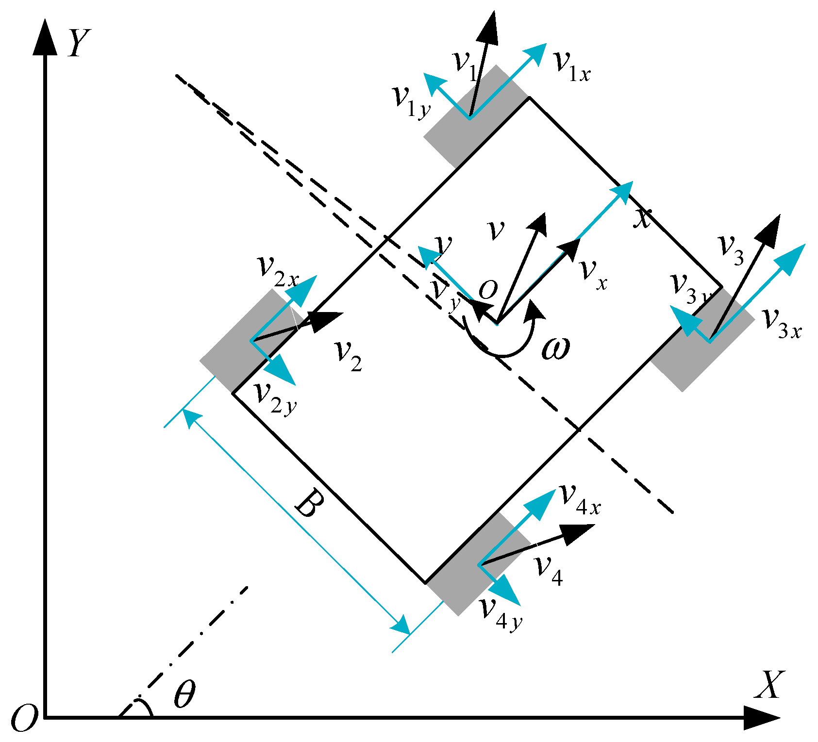
To formulate the 3-DOF kinematic model of the intelligent sweeper, a global coordinate system {O-XYZ} is introduced, together with a vehicle body coordinate system {o-xyz}, where the origin {o} is located at the vehicle’s center of mass. Both coordinate systems are defined according to the right-hand rule. In order to simplify the establishment of the four-wheel differential kinematic model, this study makes the following assumptions during the model construction process:

• It is assumed that the vehicle is a rigid body and does not undergo elastic deformation;
• In order to avoid complex friction dynamics modeling between the tire and the ground, it is assumed that only pure rolling occurs at the contact point between the tire and the ground, and lateral slip is not considered;
• In order to focus on path planning and tracking control at the kinematic level, dynamic effects such as vehicle inertia and tire deformation are ignored in the model building process.

The kinematic model of the intelligent sweeper can be expressed as follows:

Let the pose of the intelligent sweeper in the global coordinate system be denoted as ${\left(\begin{array}{c}x,y,\phi \end{array}\right)}^{\mathrm{T}}$, and its velocity in the body coordinate system be denoted as ${\left(v,\omega \right)}^{\mathrm{T}}$. Based on the geometric relationships shown in Figure 1, the velocity components in the body coordinate system are transformed into the corresponding longitudinal velocity, lateral velocity, and yaw rate in the global coordinate system. By neglecting the lateral velocity, the kinematic differential equations of the system can be formulated as follows [22]:

$$\left\{\begin{array}{l}\dot{x}=\nu \cos \theta \hfill \\ \dot{y}=\nu \sin \theta \hfill \\ \dot{\theta }=\omega \hfill \end{array}\right.$$

(1)

In the equations, v represents the linear velocity of the intelligent sweeper, ω is the yaw rate, and θ is the yaw angle.

According to the kinematic constraints, the relationship between the linear velocity v, angular velocity ω, and the velocities of the left and right drive wheels can be expressed as:

$$\left\{\begin{array}{c}\omega =\dot{\theta }={\displaystyle \frac{v_r-v_l}{B}}\\ v={\displaystyle \frac{v_r+v_l}{2}}\end{array}\right.$$

(2)

In the equation, v_r represents the velocity of the right-side drive wheel of the intelligent sweeper, v_l represents the velocity of the left-side drive wheel, and B is the distance between the centers of the two wheels.

Figure 1. Kinematics model of vehicle.

Figure 1. Kinematics model of vehicle.

2.2. Flatness Property: A Short Summary

Flatness in systems theory is a system property that extends the notion of controllability from linear systems to nonlinear dynamical systems. A system that has the flatness property is called a flat system. Flat systems have a (fictitious) flat output, which can be used to explicitly express all states and inputs in terms of the flat output and a finite number of its derivatives. This is summarized and explained in detail below [23].

Consider the system:

$$\dot{x}=f(x,u)$$

(3)

where, $x=(x_1,\dots ,x_n)\in {\mathbf{R}}^n$, $u=(u,\dots ,u_m)\in {\mathbf{R}}^m$. It is said to be (differentially) flat if, and only if:

1. There exists a vector-valued function h such that:

$$y=h(x,u,\dot{u},\dots ,u^{(r)})$$

(4)

where, $y=(y,\dots ,y_m)\in {\mathbf{R}}^m$, $r\in \mathbf{N}$;

2. The components of x = (x,…, x_n) and u = (u,…,u_m) may be expressed as:

$$x=A\left(y,\dot{y},\dots ,y^{(r_x)}\right), r_x\in \mathbf{N}$$

(5)

$$u=B\left(y,\dot{y},\dots ,y^{(r_u)}\right), r_u\in \mathbf{N}$$

(6)

If the above conditions hold at least partially, then the (possibly virtual) output is called a flat output and the system is a flat system.

2.3. A Proof of Flatness

Select the position in global coordinates as flat output:

$$y_f(t)=\left[\begin{array}{c}{y}_1(t)\\ y_2(t)\end{array}\right]=\left[\begin{array}{c}x(t)\\ y(t)\end{array}\right]$$

(7)

The first-order derivative of the system can be obtained as:

$${\dot{y}}_f(t)=\left[\begin{array}{c}\dot{x}(t)\\ \dot{y}(t)\end{array}\right]=\left[\begin{array}{c}v\cos \theta \\ v\sin \theta \end{array}\right]$$

(8)

Note that as long as v ≠ 0, we can directly solve:

$$v=\sqrt{{\dot{x}}^2+{\dot{y}}^2}=\parallel {\dot{y}}_f\parallel$$

(9)

$$\theta =\arctan \left({\displaystyle \frac{\dot{y}}{\dot{x}}}\right)$$

(10)

$$\omega (t)=\dot{\theta }(t)={\displaystyle \frac{{\dot{y}}_1(t){\ddot{y}}_2(t)-{\dot{y}}_2(t){\ddot{y}}_1(t)}{{{\dot{y}}_1}^2(t)+{{\dot{y}}_2}^2(t)}}$$

(11)

In fact, the atan2 function can determine the correct angle based on the signs of both x and y, providing an unambiguous result across all four quadrants. Therefore, the state variables of the vehicle can be determined by $y_f$ and its first-order derivative.

Taking the derivative of the Formula (7) yields:

$${\ddot{y}}_f=\dot{v}\left[\begin{array}{c}\cos \theta \\ \sin \theta \end{array}\right]+v\dot{\theta }\left[\begin{array}{c}-\sin \theta \\ \cos \theta \end{array}\right]=\left[\begin{array}{c}\cos \theta -v\sin \theta \\ \sin \theta v\cos \theta \end{array}\right]\left[\begin{array}{c}\dot{v}\\ \omega \end{array}\right]$$

(12)

Note $A(\theta ,v)=\left[\begin{array}{c}\cos \theta -v\sin \theta \\ \sin \theta v\cos \theta \end{array}\right]$, we need to prove that the matrix A(θ,v) is non-singular.

The determinant of this matrix is calculated as:

$$\det A(\theta ,v)=(\cos \theta )(v\cos \theta )-(-v\sin \theta )(\sin \theta )=v$$

(13)

As long as v ≠ 0, there is det $A(\theta ,v)\ne 0$ so the matrix A is invertible.

From the above relationship, we can obtain:

$$\left[\begin{array}{c}\dot{v}\\ \omega \end{array}\right]=A^{-1}(\theta ,v){\ddot{y}}_f$$

(14)

This shows that the angular velocity ω can be expressed by the second-order derivative of $y_f$.

Since both ${\left(\begin{array}{c}x,y,\phi \end{array}\right)}^{\mathrm{T}}$ and ${\left(v,\omega \right)}^{\mathrm{T}}$ can be reconstructed by $y_f$ and its finite-order derivatives, for differential drive, the left and right wheel speeds can also be expressed by them.

By using matrix augmentation and adjoint operation methods, we not only obtain a clear expression of the system state and input, but also prove that when v ≠ 0, the kinematic model of the smart sweeper has a strict planarity property.

2.4. Model Validation

The state quantity and control quantity of the system are defined as:

$$X(t)={\left[\begin{array}{cccc}x(t)& y(t)& \dot{x}(t)& \dot{y}(t)\end{array}\right]}^{\mathrm{T}}$$

(15)

$$U(t)=\left[\begin{array}{c}{u}_1(t)\\ u_2(t)\end{array}\right]=\left[\begin{array}{c}{\ddot{y}}_1(t)\\ {\ddot{y}}_2(t)\end{array}\right]$$

(16)

Assuming the sampling period is T seconds, using the Euler discretization method, we obtain the discrete model:

$$X(k+1)=A_{k}X(k)+B_{k}U(k)$$

(17)

where $A_k=\left[\begin{array}{cccc}1& 0& \mathrm{T}& 0\\ 0& 1& 0& \mathrm{T}\\ 0& 0& 1& 0\\ 0& 0& 0& 1\end{array}\right]$, $B_k=\left[\begin{array}{cc}{\displaystyle \frac{{\mathrm{T}}^2}{2}}& 0\\ 0& {\displaystyle \frac{{\mathrm{T}}^2}{2}}\\ \mathrm{T}& 0\\ 0& \mathrm{T}\end{array}\right]$, and T is the sampling period.

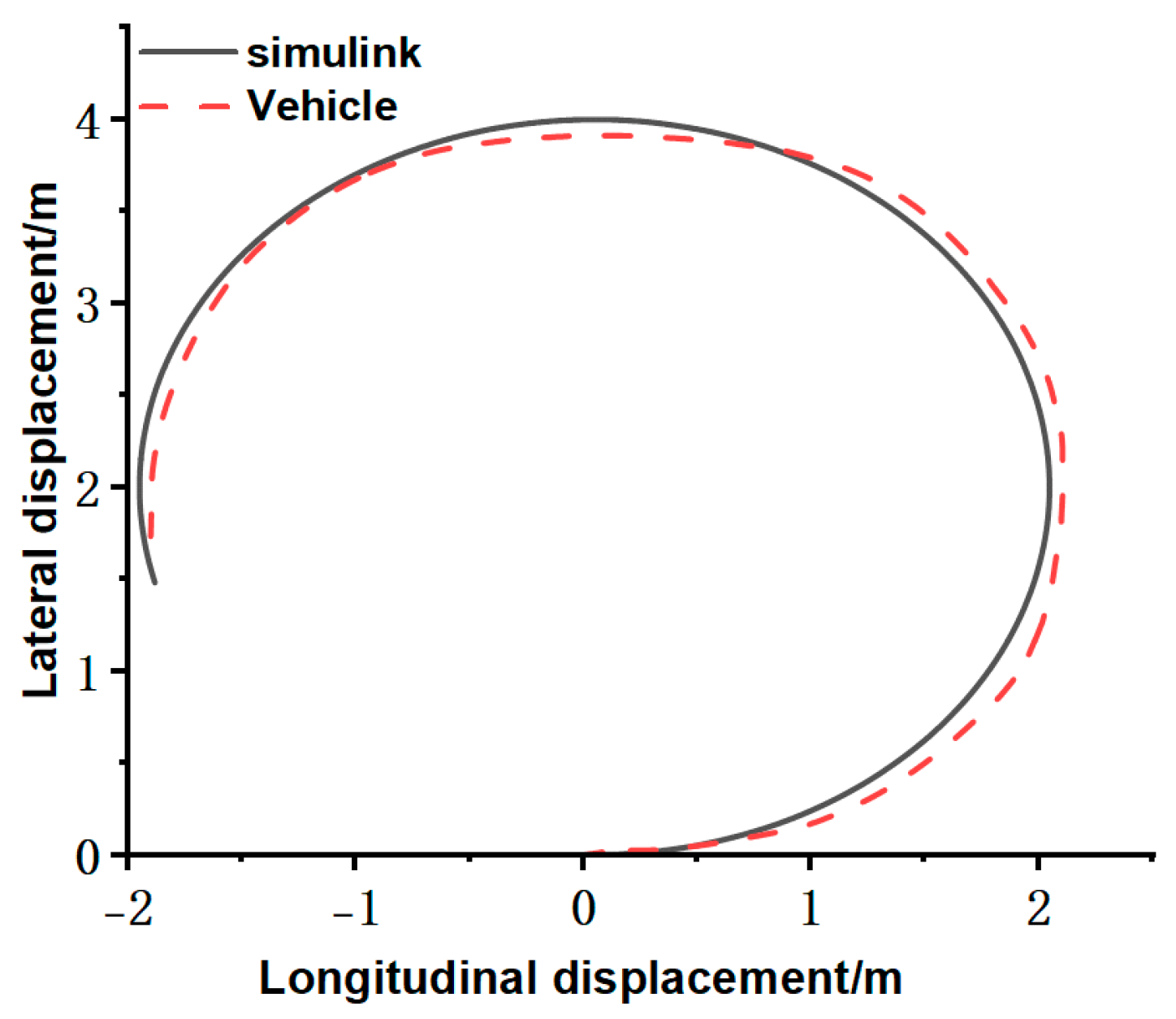
To validate the accuracy of the mathematical model for the four-wheel differential cleaning vehicle, this study employs a curved-path test by examining the variations in the tracking trajectory of the cleaning vehicle’s Simulink model at a specified wheel speed, and comparing these with the trajectory data collected from actual vehicle tests conducted under the same wheel speed conditions. The left wheel of the vehicle is set to a fixed speed of 0.85 m/s and the right wheel to 1.15 m/s (v = 1 m/s, ω = 0.5 rad/s). Both the simulation model and the actual vehicle run for 10 s, with Figure 2 illustrating the trajectories.

Under the given wheel speed conditions, the trajectory obtained from the cleaning vehicle’s mathematical model closely corresponds to the data from the actual vehicle tests, exhibiting a similar trend of variation, although significant slip and skidding are observed in the actual tests. This validates the model’s accuracy and provides a control foundation for subsequent research.

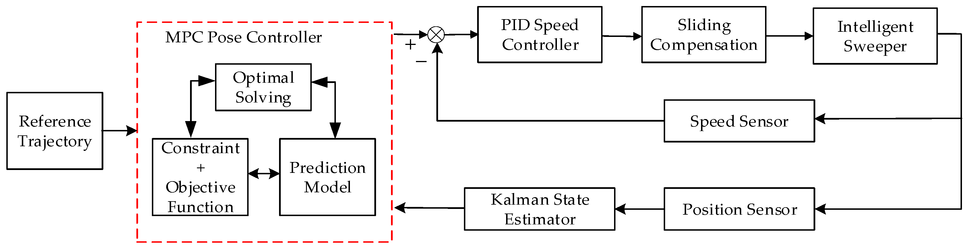
3. Dual-Loop Trajectory Tracking Control Strategy

The intelligent sweeper employs a four-wheel drive differential steering mechanism. To reduce state deviations caused by model errors and external disturbances, minimize slip errors during differential steering, and address the issues of high computational complexity and slow response time when MPC is used alone for trajectory tracking control, a parameter-corrected dual-loop trajectory tracking control strategy combining MPC and PID is proposed. In order to simplify the theoretical derivation of the controller and improve real-time performance, the design of the control strategy makes the following assumptions:

• It is assumed that the process noise and observation noise in the Kalman state estimator obey Gaussian distribution and their noise covariance matrix remains constant.
• It is assumed that during the operation of the vehicle, its inertia and the interaction characteristics between the tires and the ground remain relatively stable.
• The actual response delay of the motor or drive is not taken into account.
• In order to simplify the construction of the MPC objective function, it is temporarily assumed that the external disturbances (such as wind resistance and road unevenness) to which the vehicle is subjected during operation are small or can be ignored.

The specific system workflow is shown in Figure 3.

First, the system states are estimated. Due to the high complexity of the vehicle system, the established mathematical model inevitably contains some errors. Additionally, the sensors are highly concentrated, leading to noise affecting some controller measurements. Therefore, state estimation is essential for the system. Next, the MPC pose controller compares the position information provided by the estimator with the reference trajectory and computes the optimal control input for the current time step, which serves as the output of the outer-loop controller. Then, the difference between the target speed computed by the MPC pose controller and the current speed measured by the sensors is fed into the PID speed controller. The PID controller generates the speed control input, which serves as the output of the inner-loop controller. Finally, a sliding error compensation mechanism is applied to the control input to mitigate the impact of slip errors on the system. The compensated control input is then mapped to the drive wheel speeds through inverse kinematics to control the operation of the intelligent sweeper.

3.1. Kalman State Estimator

The traditional Kalman filter estimator assigns equal weights to all historical data, which may lead to significant errors in rapidly changing vehicle poses. To address this issue, a Forgetting Factor-based Kalman Filter (FFCKF) is introduced. By incorporating a forgetting factor, this method aims to overcome the limitations of the traditional Kalman filter when dealing with time-varying systems. Additionally, in scenarios with high noise levels or an imperfect model, it effectively smooths the estimation results, reducing fluctuations and minimizing errors. The state prediction equation is as follows:

$$\left\{\begin{array}{l}X(i+1)=AX(i)+BU(i)+W(i)\hfill \\ Z(i)=HX(i)+V(i)\hfill \end{array}\right.$$

(18)

In this equation, the state matrix A, input matrix B, state X, and control input U are consistent with the state equation in Equation (17). C represents the state observation matrix, while W and V denote the process noise and observation noise, respectively, with their corresponding covariance matrices given by Q and R.

For the system state initialization, assume the initial state is a random vector following a Gaussian distribution. The initial state and variance are given by:

$$\left\{\begin{array}{l}{\dot{X}}_0=E(X_0)\hfill \\ P_0=\mathrm{cov}(X_0,X_0^T)=E[(X_0-{\widehat{X}}_0){(X_0-{\widehat{X}}_0)}^T]\hfill \end{array}\right.$$

(19)

The state prediction equation is as follows:

$$\left\{\begin{array}{l}{\widehat{X}}^{-}(k+1|k)=A\widehat{X}(k|k-1)+BU(k|k-1)\hfill \\ \widehat{X}(k+1|k)={\widehat{X}}^{-}(k+1|k)+K_k(Z_t-H{\widehat{X}}^{-}(k+1|k))\hfill \end{array}\right.$$

(20)

By introducing a forgetting factor, the system parameters can more accurately capture changes over time, with new data being given more weight than older data. The forgetting factor λ is typically set between 0.95 and 0.995, and when λ = 1, it indicates no forgetting.

The gain of the Kalman state estimator with a forgetting factor is calculated, and the covariance of the new observation is updated as follows:

$$K_k={\displaystyle \frac{P_k^{-}{H}^T}{H{P}_k^{-}{H}^T+R}}$$

(21)

$$\left\{\begin{array}{c}{P}^{-}(k+1|k)=AP(k|k-1)A^{\mathrm{T}}+\mathrm{Q}(k)\\ P(k+1|k)={\displaystyle \frac{1}{\mathsf{\lambda }}}(1-K_{k}H)P^{-}(k+1|k)\end{array}\right.$$

(22)

Kalman filtering can be used to estimate the position and heading angle of the system by fusing the attitude information from the IMU, the localization data from the LiDAR, and the vehicle’s gyroscope signals. The measurement equation is as follows:

$$Z_k=HX(k|k)+v$$

(23)

where $H=\left[\begin{array}{cccc}1& 0& 0& 0\\ 0& 1& 0& 0\\ 0& 0& 1& 0\\ 0& 0& 0& 1\end{array}\right]$, and T is the observation matrix. The Kalman filter provides a high-precision state estimate $\widehat{X}(k)={[\widehat{x}(k),\widehat{y}(k),\widehat{\dot{x}}(k),\widehat{\dot{y}}(k)]}^T$ for subsequent MPC optimization.

3.2. MPC Pose Controller

In trajectory tracking, the MPC controller considers various factors such as the vehicle’s kinematic properties, road constraints, and obstacle information to optimize the vehicle’s trajectory and pose. It offers significant advantages in multivariable control and constraint handling [24].

From Equation (17), the estimated value of the current vehicle state can be obtained. The state variables along the vehicle’s reference trajectory satisfy the vehicle’s kinematic equation in Equation (1), so the vehicle state error is expressed as:

$$\dot{\tilde{X}}(k+1)=\left[\left.\dot{\widehat{X}}(k+1)-{\dot{X}}_{ref}(k+1)\right]\right.=A_k\tilde{X}(k)+B_k\tilde{u}(k)$$

(24)

To limit the control increment within each sampling period, thus preventing abrupt changes in the control input and ensuring the feasibility of the control process, the control increment is used instead of the control input. This approach directly limits the control increment. A new state variable can be defined as follows:

$$\xi (\mathrm{k}|\mathrm{k})=\left[\begin{array}{c}\tilde{X}(k|k)\\ \tilde{u}(k-1|k)\end{array}\right]$$

(25)

Thus, a new state-space representation can be obtained as follows:

$$\left\{\begin{array}{c}\tilde{\xi }(k+1|k)={\tilde{A}}_k\tilde{\xi }(k|k)+{\tilde{B}}_k△U(k|k)\\ \eta (k|k)={\tilde{C}}_k\xi (k|k)\end{array}\right.$$

(26)

where ${\tilde{A}}_k=\left[\left.\begin{array}{cc}{A}_k& B_k\\ 0& I_m\end{array}\right]\right.$, ${\tilde{B}}_k=\left[\left.\begin{array}{c}{B}_k\\ I_m\end{array}\right]\right.$, ${\tilde{\mathit{C}}}_k=\left[\begin{array}{cc}{\mathit{I}}_n& \mathbf{0}\end{array}\right]$, n is the dimension of the state vector, and m is the dimension of the control input vector.

The state at the next time step is determined by the current state and the current control input. By iteratively solving the system’s output at each time step within the prediction horizon N_p and control horizon N_c the output expression of the transformed state-space system is given by [25]:

$$Y(k)={\psi }_k\xi (k)+{\mathrm{\Theta }}_k\Delta U(k)$$

(27)

where $Y(k)={\left[\begin{array}{c}\eta (k+1) \eta (k+2)\dots \eta (k{+\mathrm{N}}_p)\end{array}\right]}^T$, $△U(k)={\left[\begin{array}{c}△u(k) △u(k+1)\dots △u(k+N_p-1)\end{array}\right]}^T$, ${\psi }_k={\left[\begin{array}{c}{\tilde{C}}_k{\tilde{A}}_k {\tilde{C}}_k{{\tilde{A}}_k}^2 \dots {\tilde{C}}_k{{\tilde{A}}_k}^{N_p}\end{array}\right]}^T$, ${\mathrm{\Theta }}_t=\left[\left.\begin{array}{cccc}{\tilde{C}}_k{\tilde{B}}_k& 0& \cdots & 0\\ {\tilde{C}}_k{\tilde{A}}_k{\tilde{B}}_k& {\tilde{C}}_k{\tilde{B}}_k& \cdots & 0\\ ⋮& ⋮& ⋮& ⋮\\ {\tilde{C}}_k{{\tilde{A}}_k}^{N_c-1}{\tilde{B}}_k& {\tilde{C}}_k{{\tilde{A}}_k}^{N_c-2}{\tilde{B}}_k& \ddots & {\tilde{C}}_k{{\tilde{A}}_k}^0{\tilde{B}}_k\\ ⋮& ⋮& ⋮& ⋮\\ {\tilde{C}}_k{{\tilde{A}}_k}^{N_p-1}{\tilde{B}}_k& {\tilde{C}}_k{{\tilde{A}}_k}^{N_p-2}{\tilde{B}}_k& \cdots & {\tilde{C}}_k{{\tilde{A}}_k}^{N_p-N_c}{\tilde{B}}_k\end{array}\right]\right.$.

The objective function acts as the predictive criterion for future forecasts in model predictive control, determining the prioritized reference metric for trajectory tracking control based on its configuration [26]. The primary goal of the model predictive control system is to ensure tracking accuracy while guaranteeing the smooth operation of the intelligent cleaning vehicle. However, control increments within the control horizon cannot be directly obtained through sensors or state estimation. Therefore, the objective function (21) is defined to derive a series of optimal control increments, with ε representing the relaxation factor [27]:

$$J=\parallel x-x_{\mathrm{ref}}{\parallel }_{Q_x}^2+\parallel y-y_{\mathrm{ref}}{\parallel }_{Q_y}^2+\parallel \Delta \ddot{x}{\parallel }_{R_x}^2+\parallel \Delta \ddot{y}{\parallel }_{R_y}^2+\rho {\epsilon }^2$$

(28)

where Q_x and Q_y are the state tracking weight matrices over the prediction horizon N_p for the x and y directions, respectively, and R_x and R_y are the control input weight matrices over the control horizon N_c for the x and y directions, respectively.

Quadratic programming is widely used to solve the model predictive control (MPC) objective optimization problem due to its efficiency and accuracy. Therefore, the objective function (21) is reformulated into the following standard quadratic form:

$$\underset{Z}{\min }{\displaystyle \frac{1}{2}}{Z}^{T}HZ+G^{T}Z$$

(29)

where $\Delta U=\left[\begin{array}{c}\Delta \ddot{x}(k)\\ \Delta \ddot{x}(k+1)\\ ⋮\\ \Delta \ddot{x}(k+N_c-1)\\ \Delta \ddot{y}(k)\\ \Delta \ddot{y}(k+1)\\ ⋮\\ \Delta \ddot{y}(k+N_c-1)\end{array}\right]$$Z=\left[\begin{array}{c}\Delta U\\ \epsilon \end{array}\right]$, $H=\left(\begin{array}{cc}2(Q^{T}QQ+R)& 0\\ 0& 2r\end{array}\right)$, $G=\left[\begin{array}{c}2{({\mathsf{\Psi }}_t\xi (k)-Y_{\mathrm{ref}})}^{\mathrm{T}}Q\mathsf{\Theta } 0\end{array}\right]$.

Since the intelligent sweeper may not clean effectively if its working speed is too fast, or may waste energy and reduce efficiency if the speed is too slow, it is essential to maintain an optimal forward speed during operation. Thus, the working speed must be constrained. Additionally, to ensure the smooth operation of the drive motor, the control input increments between consecutive cycles must also be constrained. The constraint equations are as follows:

$$\left\{\begin{array}{c}{U}_{\min }\le U(k)\le U_{\max }\\ \Delta U_{\min }\le \Delta U\le \Delta U_{\max }\\ |x(k)-x_{\mathrm{ref}}(k)|\le \Delta x_{\max }\\ |y(k)-y_{\mathrm{ref}}(k)|\le \Delta y_{\max }\\ |\theta (k)-{\theta }_{\mathrm{ref}}(k)|\le {\theta }_{\max }\end{array}\right.$$

(30)

where U_min, U_max, ΔU_min, and ΔU_max represent the minimum and maximum constraints for the control input and the control increment, respectively.

Finally, the design of the model predictive pose controller for the intelligent sweeper is formulated as an optimization problem aimed at minimizing the objective function J, thereby determining the control increment ΔU. The relationship between the control input at the current time step and the control increment is given by:

$$U(k)=U(k-1)+\Delta U(k)$$

(31)

3.3. PID Speed Controller

In speed control applications, the PID controller continuously monitors the vehicle’s actual velocity, compares it with the desired speed, and adjusts the rotational speeds of the left and right drive wheels to achieve precise velocity regulation [28].

The output of the speed controller is given by:

$$u_{\mathrm{PID}}(k)=K_{\mathrm{p}}e(k)+K_{\mathrm{i}}\mathrm{T}{\displaystyle \sum _{j=0}^{k}e(j)}+K_{\mathrm{d}}{\displaystyle \frac{e(k)-e(k-1)}{\mathrm{T}}}$$

(32)

By fine-tuning the PID controller parameters, the vehicle’s response to speed changes can be optimized, resulting in smoother and more accurate control.

3.4. Sliding Compensation

During the operation of the intelligent sweeper, when the actual speeds of the two wheels differ, the higher-speed side wheel is dragged by the lower-speed side wheel, resulting in slip at the contact point with the ground, which causes the actual speed to be lower than the theoretical speed. Conversely, the lower-speed side wheel is dragged by the higher-speed side wheel, causing the contact area with the ground to slide forward, making the actual speed greater than the theoretical speed.

Sliding compensation is a crucial control strategy that enhances control system performance in the presence of uncertainties such as sliding or friction. To address the issue of differential slip in the four-wheel drive system, error compensation is introduced into the controller, which helps reduce the impact of sliding errors on tracking accuracy. The relative speed error between the left and right wheels of the intelligent sweeper is given by:

$$e_{\Delta v}=\Delta v-\Delta v^{\prime }$$

(33)

where v is the theoretical speed and v′ is the actual speed.

In order to suppress the slip error caused by the wheel speed difference, the compensation term is introduced:

$$u_e=K{e}_{\Delta v}$$

(34)

where K is the compensation gain.

After obtaining the optimal control input for the current time step from the dual-loop controller, the error compensation is calculated based on the control input from the previous time step and the actual control input measured at the current time step. The error compensation is then applied as follows:

$$u_c(k)=u(k)+u_e(k)$$

(35)

The compensated optimal control input is used as the execution control input for the current time step, compensating for the impact of slip and sliding on the trajectory tracking accuracy during the actual motion of the intelligent sweeper.

Finally, the optimal control input obtained from Equation (35) is mapped to the left and right wheel speeds using the mapping relationship in Equation (2) to control the intelligent sweeper.

4. Simulation and Experimental Validation

In order to fully verify the trajectory tracking performance of the vehicle, this paper adopts a relatively complex double lane change scenario as the test condition. For the proposed MPC-PID dual closed-loop control strategy, the traditional MPC and the new RMPC algorithm proposed in the literature [15] are selected as the comparison benchmarks: the traditional MPC, as a classic predictive control framework, can intuitively reflect the performance boundary of the basic algorithm; the literature [15] is a recent new achievement, which constructs a disturbance suppression mechanism based on the robust optimization theory, and realizes the coordinated control of the longitudinal speed while optimizing the trajectory tracking accuracy. It has a high technical relevance to the coupling control problem studied in this paper. Through the quantitative comparison of indicators such as lateral tracking error, heading angle deviation, and speed response time, we can deeply analyze the response speed advantage of the dual closed-loop adaptive mechanism over the traditional single-loop MPC, and the improvement of trajectory tracking control capability compared with the complex robust optimization method, so as to systematically verify the breakthrough of the comprehensive performance of the control accuracy and real-time performance of the method in this paper in a unified experimental scenario.

Table 1. Parameters of intelligent sweeper.

Variable Name	Unit	Value
Vehicle Mass (In-house developed cleaning vehicle)	kg	37.2
Gravitational Acceleration	m·s−2	9.8
Moment of Inertia	kg·m2	7.39
Tire Rolling Radius	m	0.11
Track Width	m	0.6
Wheelbase	m	0.8
Desired Longitudinal Acceleration	m·s−2	0
Prediction Horizon	-	30
Control Horizon	-	20

shows the parameters of the intelligent sweeper.

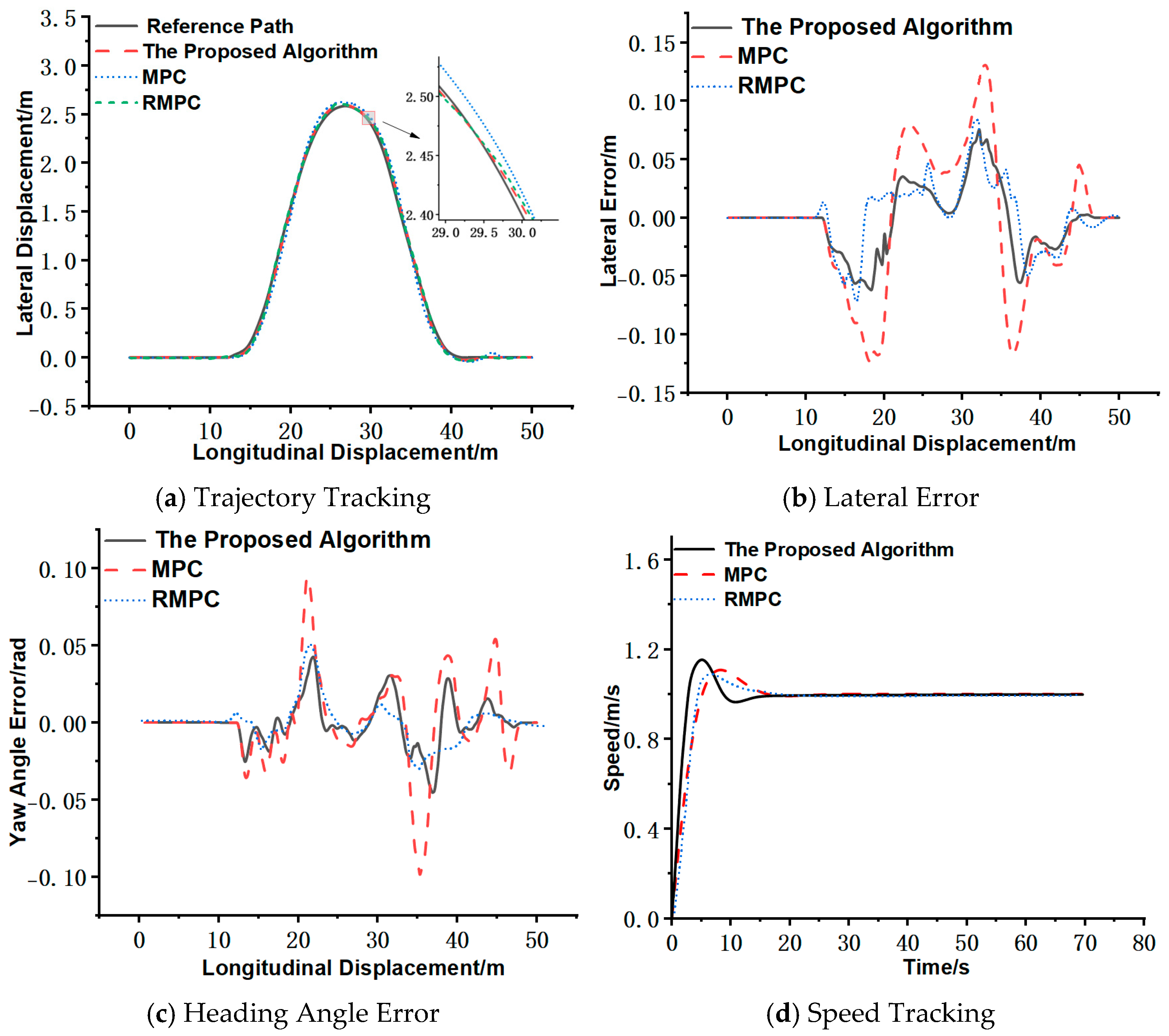
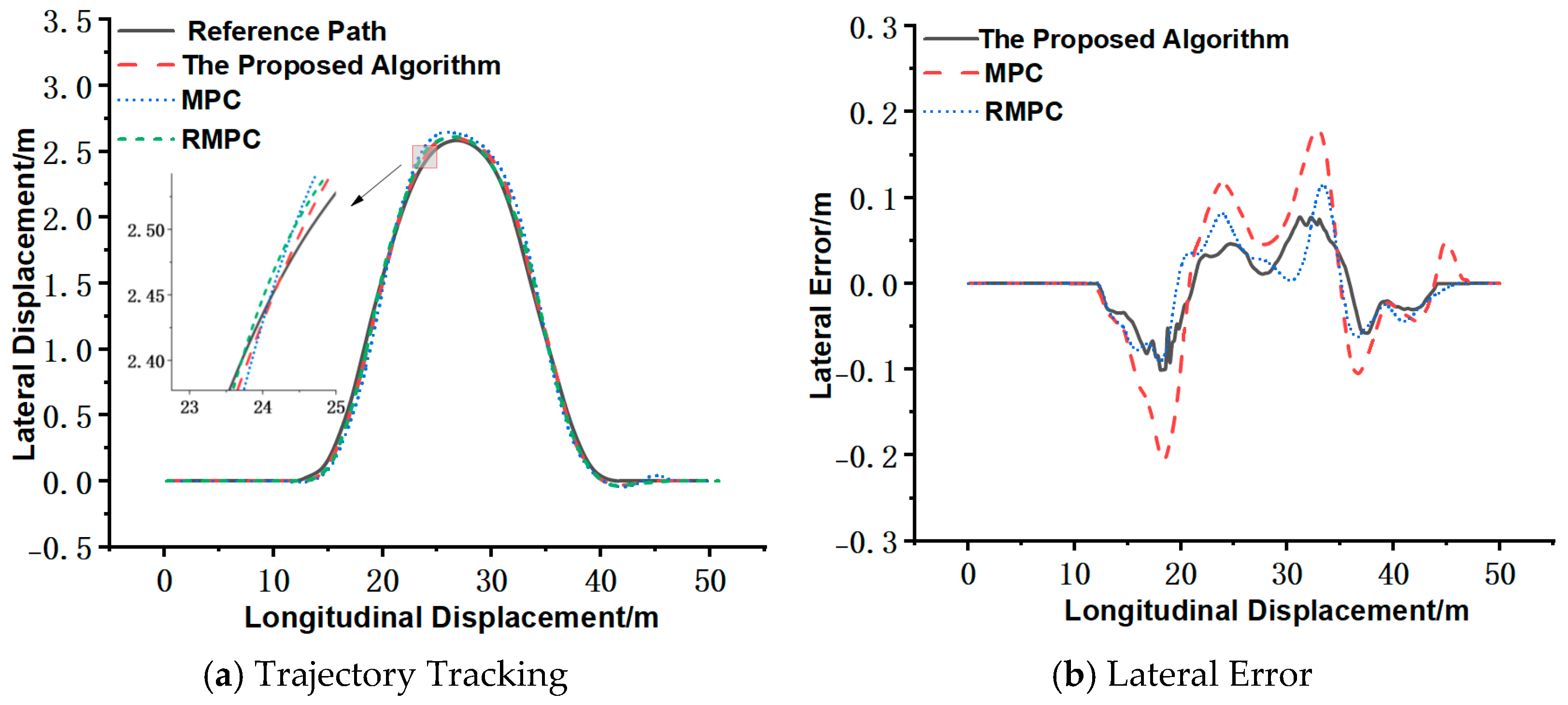
4.1. Operating Condition 1: Sweeping Operation Condition

Operating Condition 1 refers to the sweeping operation, where the sweeper operates at a speed of 3.6 km/h. The simulation results are presented in Figure 4.

Under this operating condition, Figure 4a shows that the MPC-PID algorithm proposed in this paper significantly outperforms the traditional MPC algorithm and the advanced reference algorithm RMPC in trajectory tracking performance, closely aligning with the reference trajectory. As shown in Figure 4b, the maximum lateral deviation between the trajectory tracked by the proposed controller and the reference trajectory is 0.0713 m, compared to 0.0831 m for the RMPC controller and 0.1450 m for the traditional MPC controller. Figure 4c indicates that the maximum heading angle error between the trajectory tracked by the proposed controller and the reference trajectory is 0.0445 rad, while the corresponding values for the RMPC controller and traditional MPC controller are 0.0511 rad and 0.0960 rad, respectively. Figure 4d demonstrates that the speed response time of the proposed controller is 15.18 s, whereas the RMPC controller and traditional MPC controller require 16.14 s and 16.34 s, respectively.

Table 2. Summary of experimental results under the sweeping model.

Symbol	MPC-PID	RMPC	MPC
ey_IAE	1.4372	1.3533	2.9362
ey_ITAE	51.632	55.5847	114.2585
ey_ISE	0.0525	0.0629	0.2349
eθ_IAE	0.6132	0.7851	1.2443
eθ_ITAE	25.9214	28.6569	53.4854
eθ_ISE	0.0138	0.0193	0.0583
ev_IAE	1.0298	1.7973	1.7881
ev_ITAE	5.4764	18.4374	7.3739
ev_ISE	0.7646	0.9211	0.5863

is a summary of the experimental results under the cleaning mode.

Based on experimental data analysis, significant performance differences emerge among MPC-PID, RMPC, and traditional MPC methods in low-speed trajectory tracking control (1 m/s) for intelligent sweepers. Comparative error metrics reveal that RMPC demonstrates optimal performance in steady-state tracking accuracy and terminal stability, as its robust model predictive mechanism effectively suppresses system disturbances. Conversely, MPC-PID exhibits advantages in dynamic event response, validating the adaptability of its PID compensation mechanism to sudden operational conditions. Notably, the traditional MPC shows the maximum integral absolute error (IAE), exceeding RMPC and MPC-PID by 104.3% and 116.9%, respectively. This anomalous peak highlights inherent limitations of traditional MPC in low-speed scenarios, where wheel slip and skid phenomena induce path tracking errors that persistently accumulate with path curvature variations. Therefore, the proposed algorithm achieves significant improvements in trajectory tracking accuracy and speed response time for the intelligent sweeper operating at 3.6 km/h, while maintaining computational efficiency superior to RMPC under equivalent hardware constraints.

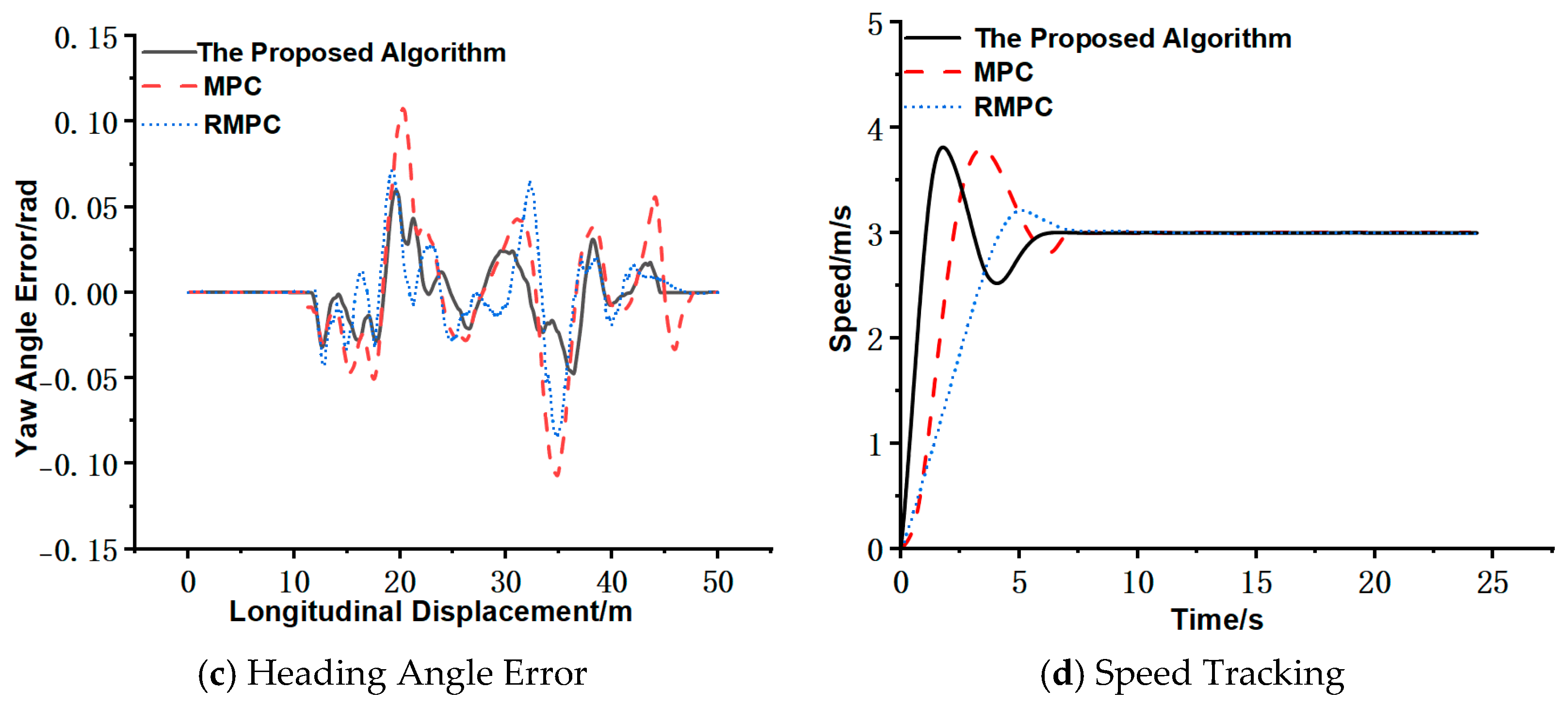
4.2. Operating Condition 2: Non-Operational Driving Condition

Operating Condition 2 refers to the normal driving speed of the sweeper, which is 10.8 km/h. The simulation results are shown in Figure 5.

Under high-speed operating conditions (10.8 km/h), Figure 5a–c demonstrate that the trajectory tracked by the traditional MPC algorithm exhibits frequent steering oscillations during curve tracking, inducing wheel slip and skid phenomena that result in significant tracking errors. In contrast, the proposed algorithm maintains robust trajectory tracking performance at this speed. As shown in Figure 5b, the maximum lateral deviation between the trajectory tracked by the proposed controller and the reference trajectory is 0.0937 m, compared to 0.1013 m for RMPC and 0.1604 m for traditional MPC. Figure 5c reveals that the maximum heading angle error reaches 0.0586 rad for the proposed controller, while RMPC and traditional MPC exhibit 0.6051 rad and 0.1076 rad, respectively. Notably, the speed response time shown in Figure 5d demonstrates the proposed controller’s superior performance at 5.68 s, significantly outperforming both RMPC (16.09 s) and traditional MPC (7.49 s). These results confirm that the proposed algorithm substantially enhances trajectory tracking precision and dynamic response capability for intelligent sweepers operating at 10.8 km/h.

Table 3. Summary of experimental results under non-sweeping mode.

Symbol	MPC-PID	RMPC	MPC
ey_IAE	0.6364	0.6930	1.2852
ey_ITAE	8.2757	9.0407	16.6717
ey_ISE	0.0368	0.0412	0.1417
eθ_IAE	0.2647	0.3430	0.5511
eθ_ITAE	3.4976	4.6061	7.5211
eθ_ISE	0.0071	0.0131	0.0288
ev_IAE	3.3124	6.0783	7.3343
ev_ITAE	6.3143	15.3899	13.5814
ev_ISE	5.6575	7.1469	15.0227

is a summary of the experimental results under non-sweeping mode.

Based on experimental data, a multi-metric comparative analysis was conducted to evaluate trajectory tracking performance for the intelligent sweeper. Error metrics reveal that the MPC-PID method demonstrates exceptional dynamic error suppression, with its Integral Absolute Error (IAE) reduced by 8.2% and 50.5% compared to RMPC and traditional MPC, respectively. This validates the effective regulation capability of the PID compensation module during high-speed dynamic processes. However, RMPC maintains superiority in longitudinal steady-state accuracy, highlighting the theoretical advantages of robust model predictive control in parameter perturbation rejection. Notably, traditional MPC exhibits significant outliers across multiple metrics, particularly in the Integral Time-weighted Absolute Error (ITAE), which exceeds MPC-PID and RMPC by 101.5% and 84.4%, respectively. This phenomenon exposes inherent deficiencies in its slip prevention mechanism, leading to persistent divergence between predicted trajectories and actual dynamic responses.

Simulation experiments at various speeds validate the adaptability of the proposed algorithm. As shown in Figure 4, under the sweeping operation condition, the proposed controller outperforms the traditional MPC controller, with improvements of 50.83% in maximum lateral deviation, 53.65% in maximum heading angle deviation, and 7.10% in speed response time. According to Figure 5, under normal driving speed, these improvements are 41.58%, 45.54%, and 24.17%, respectively. The simulation results demonstrate that the MPC-PID controller exhibits superior trajectory tracking accuracy and faster speed response across different speed conditions, significantly outperforming the traditional MPC controller.

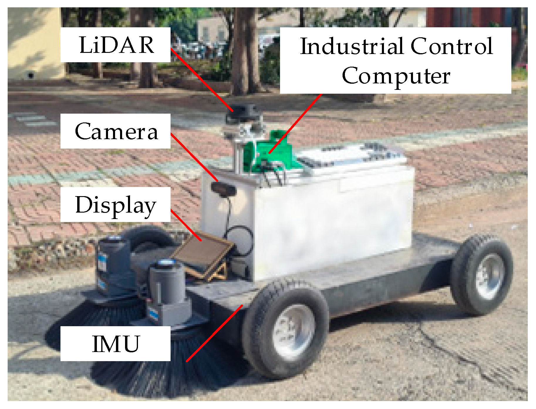
4.3. Experimental Validation

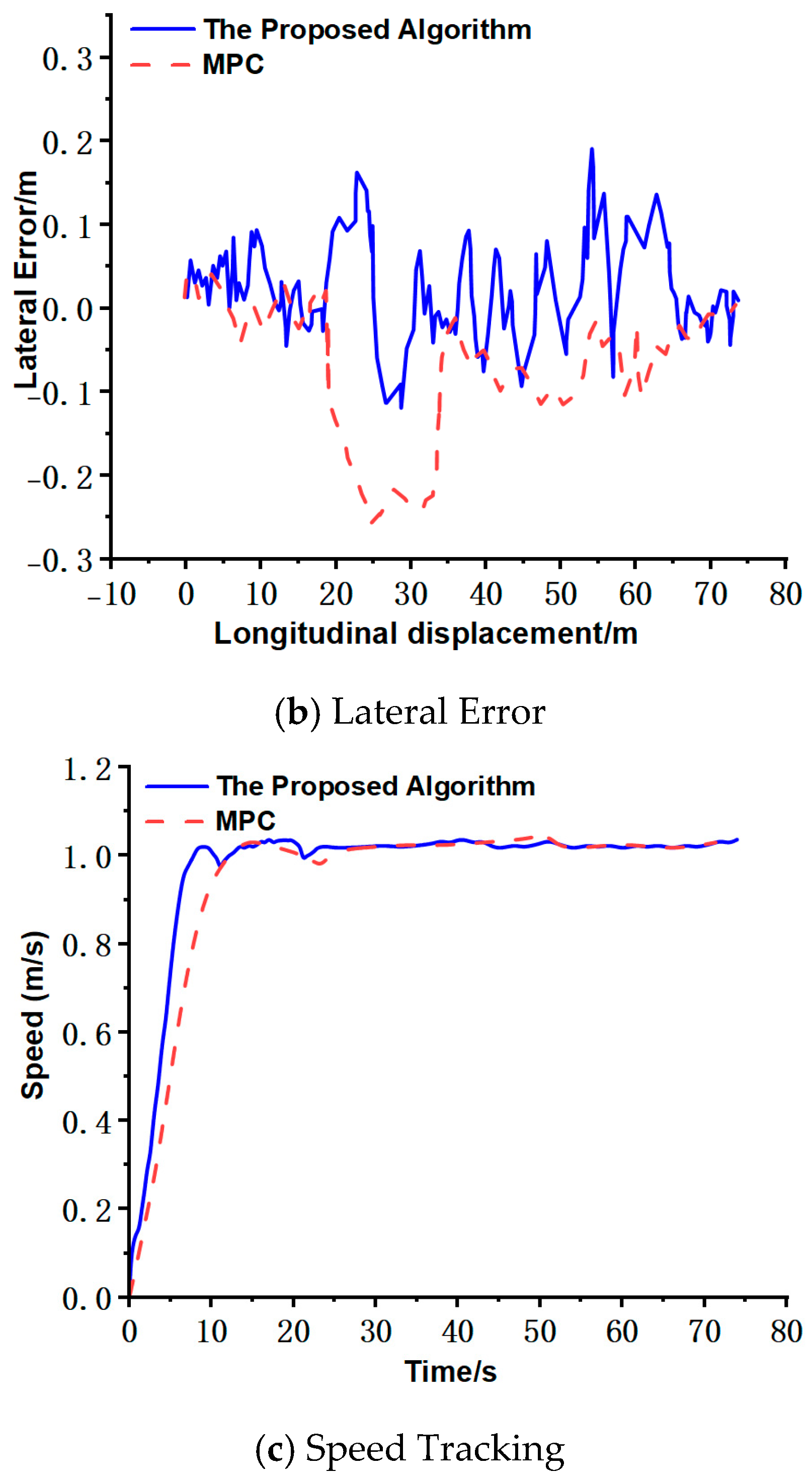
Figure 6 illustrates the intelligent sweeper, which features a fully electronic-controlled chassis, four-wheel independent drive, and differential steering. The system employs an NVIDIA Jetson Nano B01 (Santa Clara, CA, USA) as the upper computer, responsible for sensor data acquisition, processing, and computation, and outputs control commands. The lower computer, an STM32 microcontroller (Geneva, Switzerland), ensures precise control of the drive motors and the sweeping system. The real vehicle is tested on campus concrete pavement at a constant speed of 3.6 km/h. Sensor data, including an inertial measurement unit (IMU) and odometry, are collected to validate the trajectory tracking performance of the intelligent sweeper.

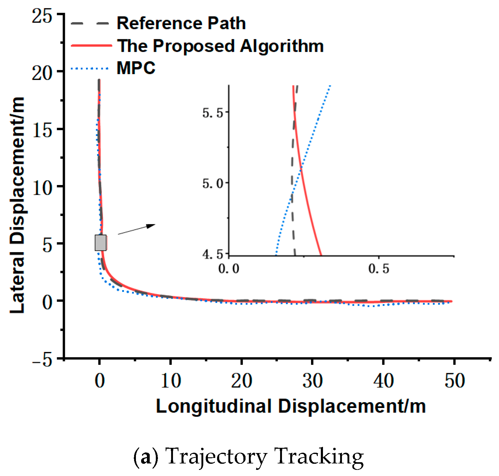
Experimental verification was conducted on campus road sections with typical operational paths consisting of straight segments and turning arcs for intelligent sweepers. Field tests demonstrate that the proposed algorithm achieves lateral tracking errors ranging from −0.139 m to 0.223 m, while traditional MPC exhibits larger error fluctuations between −0.267 m and 0.063 m. Notably, significant wheel slip and skid phenomena were observed during turns with traditional MPC, resulting in its maximum lateral deviation being 16.48% greater than our method. The proposed algorithm maintains stable speed control within 12.86 s, achieving 9.52% faster stabilization compared to traditional MPC’s 14.213 s response time, demonstrating superior steady-state performance. These results validate the simulation findings and confirm the algorithm’s effectiveness in delivering precise trajectory tracking and rapid speed response on concrete pavement surfaces. Figure 7 shows the actual vehicle test results.

5. Conclusions

To enhance the flexibility of the intelligent sweeper’s four-wheel drive differential steering system, a collaborative system integrating an MPC pose controller with a PID speed controller was designed. This system, supported by a Kalman state estimator and sliding compensation strategy, achieves high-precision, fast-response trajectory tracking control. The use of a Kalman filter for multi-sensor data fusion improves vehicle state estimation accuracy and reduces errors caused by sensor noise and external disturbances. The combination of MPC and PID speed controllers optimizes the vehicle’s pose control, improving speed accuracy during dynamic control while reducing speed response time. Sliding compensation further enhances trajectory tracking precision. Both simulation and experimental testing validated the effectiveness of the proposed MPC-PID trajectory tracking control algorithm.

Specifically, compared to conventional single-loop MPC control, this method demonstrates significant improvements in maximum lateral deviation, heading angle deviation, and speed response time. However, the experiments also revealed some limitations in the dual-loop controller. Due to the complex interactions among the controller parameters, improper tuning may result in sluggish responses or overshooting, thereby affecting the overall system robustness as well as its reliance on sensor data and the limitations of state estimation.

Therefore, it is recommended to incorporate a real-time trajectory tracking optimization control system based on multi-sensor fusion in future intelligent cleaning vehicle products. Specifically, by integrating multiple sensors for high-precision real-time monitoring of vehicle pose and velocity, and employing an advanced MPC-PID dual-loop control strategy, the system can actively adjust vehicle states to effectively compensate for motion deviations caused by external disturbances and uneven road surfaces. Additionally, it is recommended to optimize the chassis design in future products, such as lowering the vehicle’s center of gravity and adding a suspension system, to further enhance stability and disturbance resistance in complex operating environments. This study still has several issues that warrant further investigation. For example, the experimental scenarios primarily focused on ideal flat surfaces, without considering the vehicle’s motion characteristics on slopes or uneven terrain. Additionally, the current control strategy emphasizes dynamic speed response and pose accuracy, while the impact of lateral center-of-mass shifts caused by uneven load distribution has not yet been thoroughly explored. Future research will further expand the experimental scenarios, comprehensively considering sensor noise, state estimation errors, and vehicle dynamic characteristics across diverse operating conditions. The goal is to refine the proposed control approach for better real-world performance, enhancing the overall functionality and practical value of the intelligent cleaning vehicle. Additionally, adaptive algorithms will be explored for dynamic parameter optimization, and controller design will leverage system flatness (differential flatness) to improve trajectory tracking precision and robustness.