Research on Active Avoidance Control of Intelligent Vehicles Based on Layered Control Method

Abstract

To meet the active avoidance requirements of intelligent vehicles, this paper proposes an efficient hierarchical control system. The upper layer generates a safe avoidance trajectory through an optimized path planning algorithm, while the lower layer precisely controls the vehicle to follow the planned path. In the upper layer design, an improved quintic polynomial method is employed to generate the baseline trajectory. By dynamically adjusting lane change duration and utilizing an improved dual-quintic algorithm, collisions with preceding vehicles are effectively avoided. Additionally, a genetic algorithm is applied to automatically optimize parameters, ensuring both driving comfort and planning efficiency. The lower layer control is based on a three-degree-of-freedom monorail vehicle model and the Magic Formula tire model, employing a model predictive control (MPC) approach to continuously correct trajectory deviations in real time, thereby ensuring stable path tracking. To validate the proposed system, a co-simulation environment integrating CarSim, PreScan, and MATLAB was established. The system was tested under various vehicle speeds and road conditions, including wet and dry surfaces. Experimental results demonstrate that the proposed system achieves a path tracking error of less than 0.002 m, effectively reducing accident risks while enhancing the smoothness of the avoidance process. This hierarchical design decomposes the complex avoidance task into planning and control, simplifying system development while balancing safety and real-time performance. The proposed method provides a practical solution for active collision avoidance in intelligent vehicles.

1. Introduction

In recent years, with the increasing maturity of intelligent vehicle control technology and the continuous improvement of drivers’ requirements for safety, maneuverability, and ride comfort, the vehicle active avoidance problem has become one of the hotspots of research in the field of intelligent vehicle active safety [1]. Active avoidance is divided into two stages: the first stage is avoidance path planning, which is based on sensors and other devices to sense the spatial obstacles encountered while traveling and plan the optimal path from the starting point to the target point for the intelligent vehicle in advance or real-time under the condition of satisfying the dynamics, kinematics constraints, and the evaluation indexes such as stability and comfort [2]; the second stage is the avoidance path tracking, which is one of the core technologies of the intelligent vehicle, by controlling the longitudinal direction of the vehicle. One of them is to track the planned path by controlling the vehicle’s longitudinal speed and steering wheel angle, to minimize the lateral distance and direction difference between the vehicle and the target path, and at the same time, to ensure the driving stability of the intelligent driving vehicle [3].

1.1. State of Path Planning Research

According to the different ways of generating paths, path planning algorithms can be generally classified into planning methods based on graph search, planning methods based on curve interpolation, planning methods based on spatial sampling, and planning methods based on group intelligent optimization [4]. Algorithms based on graph search are mainly A* algorithm and Dijkstra algorithm. The Dijkstra algorithm is suitable for trajectory tracking control, starting from the initial point and expanding outward layer by layer until all nodes are traversed, obtaining the shortest distance from the starting point to each node. However, Dijkstra’s algorithm requires traversing the neighbors of each node, resulting in a high time complexity [5]. A* algorithm adds a heuristic function based on Dijkstra algorithm, and under the guidance of the heuristic function, the shortest path can be searched, but due to the existence of more path turning points, so there are more twists and turns, and the path is difficult to execute [6]. State spatial sampling algorithms are mainly the Rapidly exploring Random Tree (RRT) algorithm and the Probabilistic Roadmap Method (PRM), as such algorithms can randomly sample and generate collision detection paths in a large, high-latitude space, but since RRT algorithms randomly select path nodes, they cannot guarantee that the planned paths are optimal [7]. Motion space sampling algorithms, such as the CVM algorithm and the DWA algorithm, enable equidistant sampling in the velocity space. By utilizing an evaluation function, the optimal control command is selected to guide vehicle motion [8]. Wei Zhou et al. [9] constructed a path planning and tracking control framework using improved RRT and Linear Time-Varying Model Predictive Control (LTV-MPC), which realizes the effective docking between the path planning layer and the tracking control layer. Mingbo Du [10] developed a continuous curvature RRT (Continues-Curvature RRT, CC-RRT) path planning method by choosing reasonable metric function nodes. In the literature [11], RRT* is combined with sparse-RRT (sparse-RRT) to quickly converge to the optimal solution by RRT*, and at the same time reduce the computational effort by utilizing the sparsity property brought about by pruning useless nodes.

Among the intelligence optimization, the representative ones are the genetic algorithm, particle swarm algorithm, ant colony algorithm, and so on. The basic idea of the Genetic Algorithm (GA) is to start with an initial population and continuously optimize it through the simulation of natural selection, crossover, and mutation [12]. Reference [13] addresses the issues of premature convergence and slow convergence in mobile robot path planning by proposing an improved genetic algorithm that integrates an octree with a guiding function, thereby enhancing convergence speed and optimization efficiency. Reference [14] proposed an improved ant colony algorithm for the path planning problem of the AGV intelligent parking system and introduced a fallback strategy in the ant colony algorithm to improve the search efficiency of the ant colony algorithm for effective paths. Reference [15] proposed a particle swarm optimization algorithm for the impact problem of intelligent vehicle navigation paths due to the simultaneous occurrence of time-varying target behaviors and avoidance behaviors, which avoids the navigation path conflicts by optimizing the heading angle and the path speed weighting coefficients. The curves in the curve interpolation planning algorithm mainly include Bezier curves [16], polynomial curves [17] and so on. The method can construct the curve in advance, according to the current and expected state of the vehicle as a known quantity, substituting into the algorithm for parameter solving, to obtain the relevant parameters constituting the curve, the solving process to consider the road constraints and vehicle dynamics constraints, etc., and its computational volume is small and adaptable. Reference [18] uses the 3-D Bezier. The avoidance curve is first designed by path planning, and then speed planning is carried out to make the lane changing process satisfy some columns of constraints, but the method will ignore part of the vehicle’s kinematics and dynamics performance. Guochen Niu et al. [19] improved the quintuple polynomial planning algorithm with dynamic planning of lane changing time and increasing comfort constraints, on this basis, the transit state is calculated by combining the current environment and the beginning and end states of lane changing, and the twice improved quintuple polynomial algorithm is used to avoid collision with the vehicle in front of the vehicle. Yang Sun [20] compared the performance of lane changing trajectories studied by other scholars and finally concluded that the comprehensive performance of lane changing trajectories using quintic polynomial planning is optimal.

In summary, quintic polynomials are widely used in path planning, to solve the above problems, in this paper, a double quintic polynomial intelligent vehicle path planning algorithm incorporating the genetic algorithm is proposed, which utilizes the genetic algorithm for real-time optimization of the parameters of the quintic polynomials, so that the algorithm can be adapted to more working conditions and increase the comfort and safety of the process of lane changing.

1.2. State of Path Tracking Research

Path tracking control algorithms are categorized into longitudinal control and transverse control: transverse control requires the calculation of the front wheel angle at the desired position of the vehicle so that the vehicle tracks the reference transverse position; longitudinal control tracks the desired speed in the longitudinal direction. The more mature tracking control algorithms include the proportional integral differential algorithm, Stanley control algorithm, linear quadratic regulator algorithm, and model predictive control algorithm [21].

Ignacio Carlucho et al. [22] proposed an adaptive multi-PID control strategy based on reinforcement learning for the mobile trolley to control the trolley path tracking, the control method has a better effect for dealing with the complex dynamic characteristics and uncertain environment, and the results of the simulation and experiments show that the trolley has a high path tracking accuracy and robustness. Xiaobo Nie et al. [23] proposed a fuzzy PID control algorithm for the lateral stability control of high-speed vehicles, which improves the stability and comfort of the vehicle path tracking and verifies the real-time and adaptability of the control strategy after a variety of working conditions in the joint simulation. Xin Wang et al. [24] proposed a fusion algorithm, which improved the calculation of wheel angle in Stanley’s algorithm based on the pure tracking algorithm and optimized the Stanley algorithm’s accuracy and the smoothness of the path. Amer Noor Hafizah et al. [25] designed Stanley’s controller with an adaptive function, and the improved controller can adapt itself to the changing speed and heading errors. After simulation experiments, the algorithm effect is more accurate than the traditional Stanley. Y Sun et al. [26] proposed a tracking control method based on feedback linearization and linear quadratic regulator under extreme conditions. A vehicle model was established for extreme environments, and feedback linearization was used to change the nonlinear vehicle system model into a simpler linearized model. The tracking controller was designed using the LQR algorithm to obtain optimal control inputs, which ensured both system stability and optimal performance of the objective. To address the impact of parameter uncertainty and external disturbances, Jian Zhang et al. [27] proposed a path tracking method based on sliding mode control (SMC). This method designs an SMC controller based on the vehicle path tracking kinematic model and error state equation and optimizes the sliding surface coefficients using a quadratic performance index optimization method. To handle the system’s time-varying characteristics and parameter variations, fractional-order calculus is introduced, improving the method into a fractional-order sliding surface and fractional-order reaching law-based SMC. Although SMC exhibits strong robustness, it has the drawback of causing severe chattering in control output.

Xianyi Xie et al. [28] proposed a model predictive control (MPC) tracking method by modifying the time domain. This approach adjusts the control time domain step size through a matrix blocking strategy and reconstructs the objective function and system constraints in quadratic programming. Compared with traditional algorithms, it reduces computational time and enhances real-time performance.

John M. Guirguis et al. [29] proposed an adaptive model predictive controller MPC to deal with trajectory tracking, which feeds back to the controller’s effectiveness through the changing mathematical model of the vehicle, making the controller more adaptive to the instantaneous state changes parameter values, comparing the Stanley controller with the MPC with fixed vehicle model, the proposed controller possesses better tracking performance than the remaining two controllers with smaller instantaneous root mean square error. Yi Wang et al. [30] proposed a control method based on the MPC principle to improve the robustness of vehicle path tracking, and the control quantity, control increment, and state quantities affecting the maneuvering stability characteristics are incorporated into the optimization of the objective function to solve the problem, and the double-shift line condition simulation test shows that the controller has good path tracking control effect and stability.

In summary, although the PID controller is a simple algorithm, it has a low degree of fitting with the passive object, resulting in lower accuracy and larger error; Stanley algorithm requires a better smoothness of the tracked path if the smoothness is not ideal, it will produce a large lateral error of the vehicle, in addition, the algorithm ignores the characteristics of the vehicle dynamics, which does not apply to complex driving environments; LQR algorithm, although it can solve for the control quantities, it cannot add external constraints, and it is difficult to constrain the vehicle’s motion state. Model predictive control is often used to deal with tracking problems, because it can add comfort and safety constraints as needed under the premise of considering the vehicle dynamics model, and it has a good control effect on the vehicle. Based on the four controllers’ applicable scenarios and solution accuracy, the MPC algorithm is selected to track the path in this paper.

The vehicle hierarchical active avoidance control architecture is shown in Figure 1, which is divided into a path planning layer and a path tracking layer. The path planning layer plans the avoidance path by using the double-fifth polynomial of the fusion genetic algorithm according to the relative position information of the obstacles obtained by the sensors and the motion state of the vehicle, and the path tracking layer takes the local avoidance path planned by the upper controller as a reference to control the steering wheel angle of the vehicle to realize the active avoidance function.

This paper decomposes the obstacle avoidance problem into two independent modules: upper layer path planning and lower layer path tracking. The upper layer is responsible for global path optimization, while the lower layer focuses on local path tracking. This modular design facilitates algorithm debugging and optimization. The upper level path planning strategy is based on a dual quintic polynomial to enhance the smoothness of the lane change path, ensure lane change safety, and meet real-time requirements [31].

The lower layer path tracking is implemented using model predictive control (MPC), which integrates the vehicle dynamic model and tire model. The objective function considers factors such as the vehicle’s centroid slip angle, road surface adhesion coefficient, and tire slip constraints to ensure vehicle dynamic stability.

The hierarchical architecture effectively decouples the complexity of planning and control. The upper layer planner focuses on generating smooth and safe avoidance paths, while the lower layer controller ensures high-precision path tracking, thereby improving the overall robustness of the system.

2. Vehicle and Tire Model

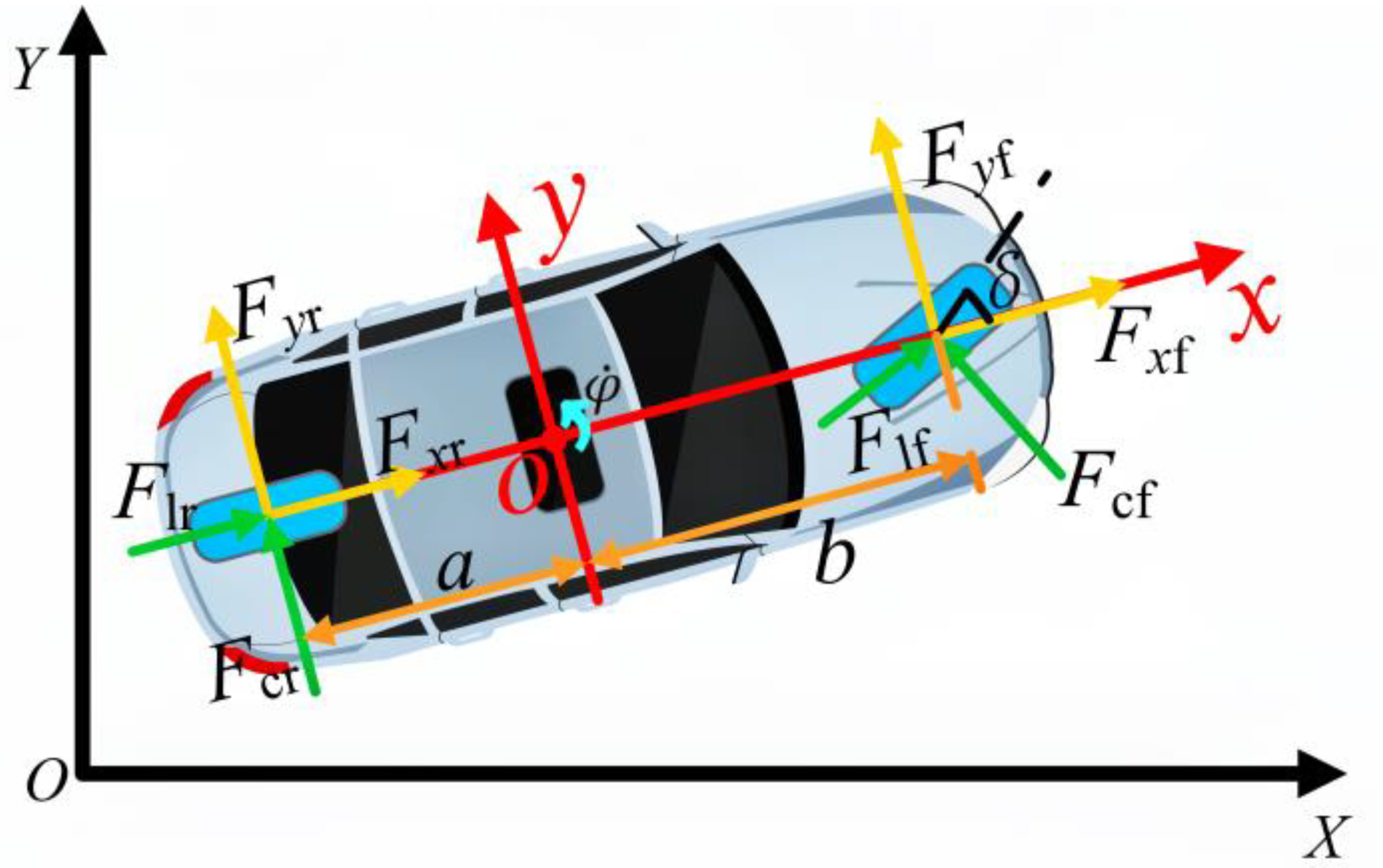
2.1. Three-Degree-of-Freedom Vehicle Dynamics Model

The path planning and tracking control of intelligent vehicles needs to be realized by combining the vehicle dynamics system, because the real vehicle has high nonlinearity, so it is difficult to depict the vehicle motion state through the state equations, so building a reasonable and simplified vehicle dynamics model is a prerequisite for vehicle dynamics control [32]. According to the needs of the control algorithm, this paper builds a three-degree-of-freedom monorail vehicle model, as shown in Figure 2, in which xoy is the vehicle coordinate system, XOY is the geodetic coordinate system, and the following assumptions are made: ignore the influence of the suspension movement on the vehicle; ignore the transfer of the front and rear axle loads in the course of the vehicle’s movement; and ignore the influence of the aerodynamics on the vehicle’s motion characteristics.

The longitudinal equation of motion of the vehicle is:

$$m\ddot{x}=m\dot{y}\dot{\phi }+2F_{xf}+2F_{xr}$$

(1)

where m is the mass of the vehicle, x is the longitudinal displacement of the vehicle, y is the lateral displacement of the vehicle, φ is the transverse angle of the vehicle, and F_xf and F_xr represent the longitudinal forces on the front and rear tires of the vehicle.

The lateral equation of motion of the vehicle is:

$$m\ddot{y}=m\dot{x}\dot{\phi }+2F_{yf}+2F_{yr}$$

(2)

where F_yf and F_yr represent the lateral forces on the front and rear tires of the vehicle.

The equation of motion for the vehicle’s transverse pendulum is:

$$I_z\ddot{\phi }=2a{F}_{yf}-2b{F}_{yr}$$

(3)

where I_z is the yaw inertia of the vehicle around the z-axis, and a and b are the distances of the center of mass from the front and rear axles.

The combined force on the tire in the x-direction and y-direction is converted to longitudinal and lateral forces in the following manner:

$$\left\{\begin{array}{l}{F}_{\mathit{xf}}=F_{\mathrm{lf}}\cos {\delta }_{\mathrm{f}}-F_{\mathrm{cf}}\sin {\delta }_{\mathrm{f}}\hfill \\ F_{xr}=F_{\mathrm{lr}}\cos {\delta }_{\mathrm{r}}-F_{\mathrm{cr}}\sin {\delta }_{\mathrm{r}}\hfill \\ F_{yf}=F_{\mathrm{lf}}\sin {\delta }_{\mathrm{f}}+F_{\mathrm{cf}}\cos {\delta }_{\mathrm{f}}\hfill \\ F_{yr}=F_{\mathrm{lr}}\sin {\delta }_f+F_{\mathrm{cr}}\cos {\delta }_{\mathrm{r}}\hfill \end{array}\right.$$

(4)

where δ_f and δ_r indicate front wheel angle and rear wheel angle, F_cf, and F_cr denote the combined lateral force on the front and rear wheels, and F_lf and F_lr denote the combined lateral force on the front and rear wheels.

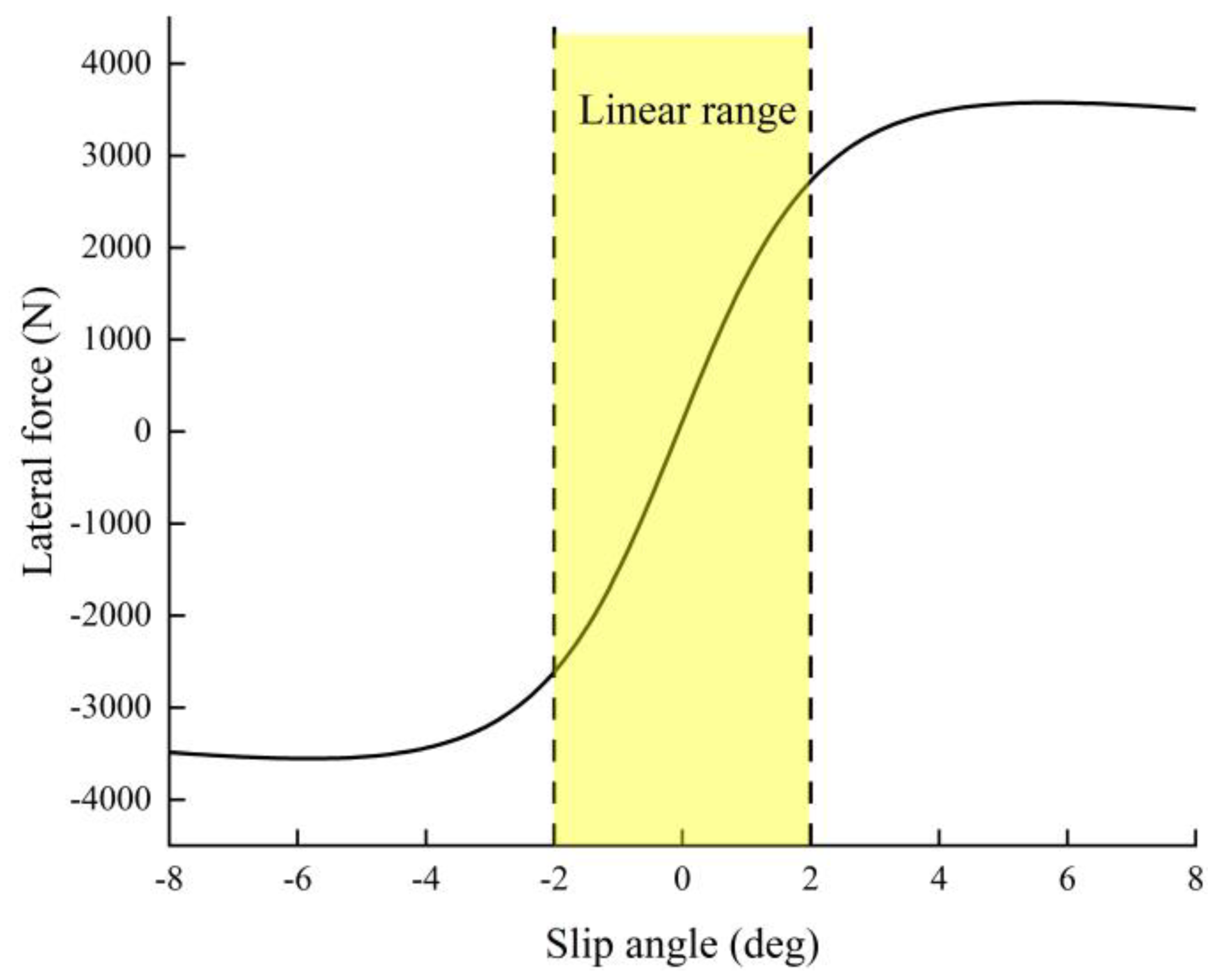
2.2. Magic Formula Tire Model

In the process of vehicle movement, the tire is the only mechanism that contacts the ground, with strong nonlinear dynamics, most of the forces affecting the vehicle characteristics come from the tire, in order to ensure the accuracy of the algorithm, this paper selects the Magic Formula tire model with higher accuracy [33].

The general expression for the magic tire formula is:

$$\left\{\begin{array}{c}Y\left(x_1\right)=D\sin \left\{C\arctan \left[B{x}_1-E\left(B{x}_1-\arctan \left(B{x}_1\right)\right)\right]\right\}+S_{\mathrm{v}}\\ x_1=\mathrm{X}+S_{\mathrm{h}}\end{array}\right.$$

(5)

where the output Y can be calculated from the parameters B, C, D, and E, where B is the stiffness factor; C is the curve shape factor; D is the curve peak factor; E is the curvature factor; x₁ is the input variable; S_h and S_v are the drift of the curve horizontally and vertically, respectively; X denotes the lateral deflection angle α of the tire or the slip rate s; and, depending on the inputs, the outputs can be expressed as the longitudinal force, the lateral force, and the backward corrective moment of the tire.

When the tires are subjected to different vertical loads, the values of each parameter in the formula change accordingly, and in order to show the relationship between them, the data fitting method is used to convert them into polynomial form to determine the value of each parameter, which is calculated by the following formula.

Calculation of longitudinal tire forces:

$$\left\{\begin{array}{c}{F}_l=D_x\sin \left\{C_x\arctan \left[B_x{x}_1-E_x\left(B_x{x}_1-\arctan B_x{x}_1\right)\right]\right\}+S_v\\ x_1=\mathrm{s}+{\mathrm{S}}_{\mathrm{h}}\end{array}\right.$$

(6)

The formula for calculating each parameter is shown below:

$$\left\{\begin{array}{l}{B}_x=\left(b_3{F}_z^2+b_4{F}_z\right)e^{-b_5{F}_z}/C_x\cdot D_x\hfill \\ C_x=b_0\hfill \\ D_x=\mu \left(b_1{F}_z^2+b_2{F}_z\right)\hfill \\ E_x=b_6{F}_z^2+b_7{F}_z+b_8\hfill \\ S_{\mathrm{v}}=0\hfill \\ S_{\mathrm{h}}=b_9{F}_z+b_{10}\hfill \end{array}\right.$$

(7)

where F_z denotes the vertical force on the wheel and μ denotes the road surface coefficient.

Calculation of tire lateral forces:

$$\left\{\begin{array}{c}{F}_c=D_x\sin \left\{C_x\arctan \left[B_x{x}_1-E_x\left(B_x{x}_1-\arctan B_x{x}_1\right)\right]\right\}+S_v\\ x_1=\alpha +S_h\end{array}\right.$$

(8)

The formula for calculating each parameter is shown below:

$$\left\{\begin{array}{l}{B}_x=a_3\sin \left[2\arctan \left(F_z/a_4\right)\right]\cdot \left(1-a_5\left|\gamma \right|\right)/\left(C\cdot D\right)\hfill \\ C_x=a_0\hfill \\ D_x=\mu \left(a_1{F}_z^2+a_2{F}_z\right)\hfill \\ E_x=a_6{F}_z+a_7\hfill \\ S_{\mathrm{h}}=a_9{F}_{\mathrm{z}}+a_{10}+a_8\gamma \hfill \\ S_{\mathrm{v}}=a_{11}{F}_{\mathrm{z}}\gamma +a_{12}{F}_{\mathrm{z}}+a_{13}\hfill \end{array}\right.$$

(9)

where γ is the camber angle of the wheel.

Calculation of wheel return torque:

$$\left\{\begin{array}{c}{\mathrm{M}}_{\mathrm{z}}=D_{\mathrm{x}}\sin \left\{C_{\mathrm{x}}\arctan \left[B_{\mathrm{x}}{x}_1-E_{\mathrm{x}}\left(B_{\mathrm{x}}{x}_1-\arctan B_{\mathrm{x}}{x}_1\right)\right]\right\}+S_{\mathrm{v}}\\ x_1=\alpha +S_{\mathrm{h}}\end{array}\right.$$

(10)

The formula for calculating each parameter is shown below:

$$\left\{\begin{array}{l}{B}_x=B_x{C}_x{D}_x/\left(C_x\cdot D_x\right)\hfill \\ C_x=c_0\hfill \\ D_x=\mu \left(c_1{F}_z^2+c_2{F}_z\right)\hfill \\ E_x=\left(c_7{F}_z^2+c_8{F}_z+c_9\right)\left(1-c_{10}\left|\gamma \right|\right)\hfill \\ B_x{C}_x{D}_x=\left(c_3{F}_z^2+c_4{F}_3\right)\left(1-c_6\left|\gamma \right|\right)e^{-c_5{F}_z}\hfill \\ S_h=c_{11}\gamma +c_{12}{F}_s+c_{13}\hfill \\ S_v=\gamma \left(c_{14}{F}_z^2+c_{16}{F}_z\right)+c_{16}{F}_z+c_{17}\hfill \end{array}\right.$$

(11)

In this paper, the selected tire model is 225/60 R18. In the equations, a₀–a₁₃, b₀–b₁₀, c₀–c₁₇ are the parameters required for factor calculations. According to the basic form of the Magic Formula, based on the given parameters, references [34,35], a part of the simulation parameters are formulated within a reasonable range, and the simulation results are obtained in Matlab, and the simulation results are shown in Figure 3 and Figure 4 below.

Figure 3 shows the relationship between tire longitudinal force and longitudinal slip rate. As shown in the figure, there is a strong nonlinear relationship between lateral force and slip rate, but when the slip rate of the tire is less than 4%, the relationship between the longitudinal force of the tire and the longitudinal slip rate becomes approximately linear. The slip rate for normal vehicle operation generally does not exceed 2%.

Figure 4 shows the relationship between the tire sidewall force and the tire sidewall angle, from which it can be seen that in the range of small angles of sidewall angle, it also becomes approximately linear. When the side deflection angle is greater than 2°, the slope of the curve becomes smaller, indicating that side slip has begun to occur at the tire ground, until the whole tire side slips.

Referring to Figure 3 and Figure 4, the vehicles that are generally in a stable driving state have their side deflection angles and slip rates in a relatively small range of variation, and the tire forces involved in this paper are all approximated by linear functions. In addition, there are a large number of trigonometric functions in the vehicle dynamics model described by Equations (1)–(3), and since the angles involved in the dynamics model are all in a small angular interval, each trigonometric function can satisfy the following approximation conditions:

$$\sin \theta \approx \theta ,\cos \theta \approx 1,\tan \theta \approx \theta$$

(12)

With the introduction of lateral deflection stiffness, longitudinal stiffness, lateral deflection angle, and slip rate, the tire force of the vehicle can be expressed as:

$$\left\{\begin{array}{l}{F}_{\mathrm{cf}}=C_{\mathrm{cf}}\left({\delta }_t-{\displaystyle \frac{\dot{y}+a\dot{\phi }}{\dot{x}}}\right)\hfill \\ F_{\mathrm{cr}}=C_{\mathrm{cr}}{\displaystyle \frac{\dot{y}-b\dot{\phi }}{\dot{x}}}\hfill \\ F_{\mathrm{lf}}=C_{\mathrm{lf}}{s}_{\mathrm{f}}\hfill \\ F_{\mathrm{lr}}=C_{\mathrm{lr}}{s}_i\hfill \end{array}\right.$$

(13)

where C_lf and C_lr denote the longitudinal stiffness of the front and rear tires, and C_cf and C_cr denote the lateral stiffness of the front and rear tires.

The nonlinear dynamic equations for a three-degree-of-freedom vehicle are derived by combining Equations (1)–(3) and (13):

$$\left\{\begin{array}{l}\mathrm{m}\ddot{\mathrm{x}}=\mathrm{m}\dot{\mathrm{y}}\dot{\mathsf{\phi }}+2\left[C_{\mathrm{lf}}{\mathrm{s}}_{\mathrm{f}}-C_{\mathrm{cf}}\left({\delta }_{\mathrm{f}}-{\displaystyle \frac{\dot{\mathrm{y}}+a\dot{\mathsf{\phi }}}{\dot{\mathrm{x}}}}\right){\delta }_{\mathrm{f}}+C_{\mathrm{lf}}{\mathrm{s}}_{\mathrm{f}}\right]\hfill \\ \mathrm{m}\ddot{\mathrm{y}}=-\mathrm{m}\dot{\mathrm{x}}\dot{\mathsf{\phi }}+2\left[C_{\mathrm{cf}}\left({\delta }_{\mathrm{f}}-{\displaystyle \frac{\dot{\mathrm{y}}+a\dot{\mathsf{\phi }}}{\dot{\mathrm{x}}}}\right)+C_{\mathrm{cr}}\left({\displaystyle \frac{b\dot{\mathsf{\phi }}-\dot{\mathrm{y}}}{\dot{\mathrm{x}}}}\right)\right]\hfill \\ I_Z\ddot{\mathsf{\phi }}=2\left[{\mathrm{aC}}_{\mathrm{cf}}\left({\delta }_{\mathrm{f}}-{\displaystyle \frac{\dot{\mathrm{y}}+a\dot{\mathsf{\phi }}}{\dot{\mathrm{x}}}}\right)-b{C}_{\mathrm{cr}}\left({\displaystyle \frac{b\dot{\mathsf{\phi }}-\dot{\mathrm{y}}}{\dot{\mathrm{x}}}}\right)\right]\hfill \end{array}\right.$$

(14)

Since the controller design is based on the geodetic coordinate system, it is necessary to convert the body coordinate system to the geodetic coordinate system, and the conversion equation is shown below:

$$\left\{\begin{array}{l}\dot{Y}=\dot{x}\sin \phi +\dot{y}\cos \phi \hfill \\ \dot{X}=\dot{x}\cos \phi -\dot{y}\sin \phi \hfill \end{array}\right.$$

(15)

Its state space expression is

$$\left\{\begin{array}{l}{\dot{\xi }}_d=f\left({\xi }_d,u_d\right)\hfill \\ {\eta }_d=h_d\left({\xi }_d\right)\hfill \end{array}\right.$$

(16)

where the state quantity is ${\xi }_d={\left[\dot{y},\dot{x},\phi ,\dot{\phi },Y,X\right]}^T$, control quantity is $u_d=\left\{{\delta }_d\right\}$, and output quantity is ${\eta }_d={\left[{\delta }_d,Y\right]}^T$.

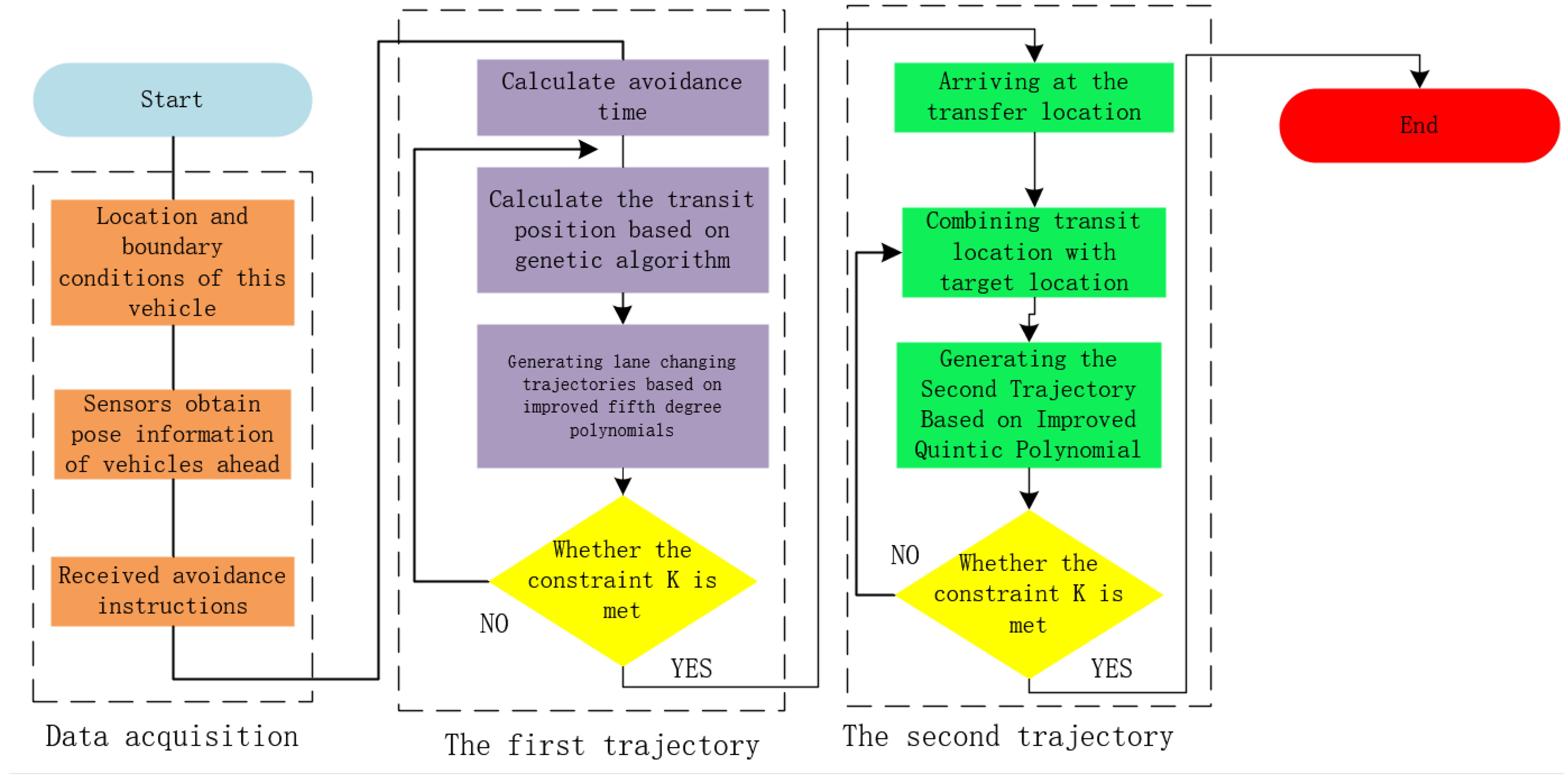
3. Double Quintic Polynomial Path Planning Incorporating Genetic Algorithms

Avoidance path planning is the basis and premise of the vehicle to complete the active avoidance, the vehicle through its own sensors and V2X communication to collect the position, speed, acceleration, and relative distance information of the vehicle and the traffic vehicle, calculating the time required for the lane change. By utilizing the improved quintic polynomial, the system can calculate the avoidance time based on the vehicle’s pose and generate the avoidance path. The midpoint position is determined using a genetic algorithm, which optimizes the parameters of the two-stage avoidance paths. This approach ensures that the planned avoidance trajectory satisfies the requirements for avoiding dynamic traffic vehicles. The schematic diagram of the vehicle avoidance process is shown in Figure 5. The vehicle senses obstacle vehicle C1 at position M and begins to avoid it. After the first movement, it reaches the transfer position M1, and after the second movement, it reaches the end of avoidance position M2.

The avoidance trajectory is shown in Figure 6. After collecting environmental data, the vehicle begins to calculate the avoidance time and generates the first segment of the trajectory. The transfer position is calculated using a genetic algorithm, and the avoidance trajectory is generated based on an improved fifth-degree polynomial, satisfying the constraint condition K. After reaching the intermediate position, a second trajectory is generated by combining the intermediate position with the target position. At the same time, the constraint condition K is met, and the double quintic polynomial avoidance trajectory is completed.

3.1. Estimated Time of Avoidance

Due to the different motion states of the traffic car, the avoidance time obtained by calculation will also have a big difference, so it is necessary to discuss the motion state of the traffic car, the traffic car motion state is divided into the following four kinds: the traffic car is stationary, the traffic car is from stationary to motion, the traffic car is moving at a constant speed, the traffic car is moving at a variable speed.

3.1.1. Traffic Vehicle Stationary

When the traffic vehicle in front is stationary, the longitudinal distance required to complete the avoidance should be less than the distance from this vehicle to the traffic vehicle, then the avoidance time T is calculated as shown below:

$$T={\displaystyle \frac{x_{\mathrm{tf}}}{v_{\mathrm{xin}}}}$$

(17)

where x_tf is the distance of the vehicle from the traffic vehicle and v_xin is the initial speed of the vehicle at the beginning of the avoidance.

3.1.2. Traffic Vehicles from Stationary to Motion

When this vehicle detects a traffic vehicle, the traffic vehicle starts moving from a standstill, and the avoidance time T is calculated as shown below:

$$T={\displaystyle \frac{v_{\mathrm{xin}}-\sqrt{v_{\mathrm{xin}}^2-2a_{\mathrm{xtf}}{x}_{\mathrm{tf}}}}{a_{\mathrm{xtf}}}}$$

(18)

where a_xtf is the acceleration of the traffic vehicle and v_xtf is the longitudinal velocity of the traffic vehicle.

3.1.3. Uniform Motion of Traffic Vehicles

Similar to a traffic vehicle that is stationary, the avoidance time T is calculated as follows when the traffic vehicle is moving at a constant speed:

$$T={\displaystyle \frac{x_{\mathrm{tf}}}{v_{\mathrm{xin}}-v_{\mathrm{xtf}}}}$$

(19)

3.1.4. Transit Vehicle Variable Speed Motion

The avoidance time T is shown below when the dynamic traffic vehicle is in variable speed motion:

$$T={\displaystyle \frac{\left(v_{\mathrm{xin}}-v_{\mathrm{xtf}}\right)+\sqrt{{\left(v_{\mathrm{xtf}}-v_{\mathrm{xin}}\right)}^2+2a_{\mathrm{xtf}}{x}_{\mathrm{tf}}}}{a_{\mathrm{xtf}}}}$$

(20)

Table 1. Avoidance times and staging locations under different road conditions.

Vehicle Speed (m/s)	Vehicle Acceleration (m/s2)	Distance Between This Vehicle and Traffic (m)	Traffic Vehicle Speed (m/s)	Traffic Vehicle Acceleration (m/s2)	First Avoidance Time (s)	Staging Post (m)
17	0	40	0	0	2.1177	35.38
17	−2	40	0	0	2.52	36.17
17	0	40	12	0	7.2	109.94
17	0	40	18	−2	6.01785	95.83
23	0	40	18	−2	3.87	85.46

shows the vehicle avoidance time and transit position under different road conditions, as shown in the table, when the speed of this vehicle is unchanged, the avoidance time and transit position change with the change in the traffic vehicle’s position, which has good real-time performance.

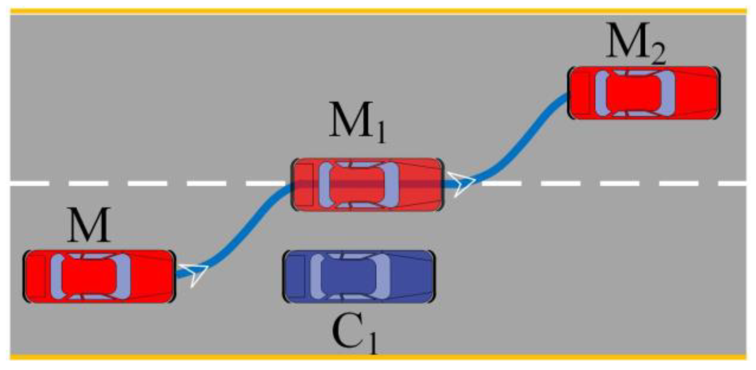
3.2. Double Quintuple Polynomial Avoidance Path Planning

The path planning function based on the fifth-degree polynomial is:

$$\left\{\begin{array}{c}x\left(t\right)=a_0+a_{1}t+a_2{t}^2+a_3{t}^3+a_4{t}^4+a_5{t}^5\\ y\left(t\right)=b_0+b_{1}t+b_2{t}^2+b_3{t}^3+b_4{t}^4+b_5{t}^5\end{array}\right.$$

(21)

where a_i, b_i are the coefficients to be determined, i = 0, 1, …, 5, and t is the time.

3.2.1. Vehicle Status Setting

In order to ensure the smooth movement of the vehicle when changing lanes, it is necessary to use the vehicle state to constrain the avoidance path, which includes longitudinal motion constraints and lateral motion constraints. Assuming that the initial state of the vehicle is (x_in,v_xin,a_xin,y_in,v_yin,a_yin), the transit state of the vehicle is (x_c,v_xc,a_xc,y_c,v_yc,a_yc), the final state of the vehicle is (x_fin,v_fin,a_fin,y_fin,v_yfin,a_yfin), and the state of the traffic vehicle is (x_tf,v_xtf,a_xtf,y_tf,v_ytf,a_ytf), with the subscripts in denoting the avoidance initial state, c denoting the avoidance transit state, and fin denoting the end state of avoidance.

In the avoidance of the initial moment, transit moment, and the end of the moment, intelligent vehicles are in the lane line smooth driving and the direction of movement parallel to the lane line, the vehicle only longitudinal speed, horizontal and longitudinal no acceleration tendency, so the initial state of the vehicle (0,v_xin,0,0,0,0,0), the transit target state (L,v_xc,0,h,0,0). From this, we can derive the Equation (21). The lane width h is 3.75 m, longitudinal displacement is L, and is located at t = t₀ when the avoidance is completed, where t₀ is the avoidance time. The values of the boundary conditions are brought into Equation (20) to obtain Equations (22) and (23).

$$\left\{\begin{array}{l}{b}_0=b_1=b_2=0\hfill \\ a_0=a_2=0\hfill \\ a_1=v_{\mathrm{xin}}\hfill \end{array}\right.$$

(22)

$$\left\{\begin{array}{l}{b}_5{t}_0^5+b_4{t}_0^4+b_3{t}_0^3=h\hfill \\ 5b_5{t}_0^2+4b_4{t}_0+3b_3=0\hfill \\ 10b_5{t}_0^2+6b_4{t}_0+3b_3=0\hfill \end{array}\right.$$

(23)

$$\left\{\begin{array}{l}{a}_5{t}_0^5+a_4{t}_0^4+a_3{t}_0^3+v_{\mathrm{xin}}{t}_0=L\hfill \\ 5a_5{t}_0^4+4a_4{t}_0^3+3a_3{t}_0^2+v_{\mathrm{xin}}=v_{\mathrm{xc}}\hfill \\ 10a_5{t}_0^2+6a_4{t}_0+3a_3=0\hfill \end{array}\right.$$

(24)

3.2.2. Constraint Establishment

To ensure the safety and comfort of the lane changing process, this paper combines the vehicle dynamics characteristics during the actual motion to constrain the longitudinal, lateral, and additive accelerations of the two avoidance paths.

(1)

Setting the longitudinal and lateral acceleration constraints for two-lane change trajectories

$$\begin{array}{l}\left\{\begin{array}{c}-2.5 \mathrm{m}/{\mathrm{s}}^2\le a_1\le 2.5 \mathrm{m}/{\mathrm{s}}^2\\ -2.0 \mathrm{m}/{\mathrm{s}}^2\le a_2\le 2.0 \mathrm{m}/{\mathrm{s}}^2\end{array}\right.\hfill \\ \end{array}$$

(25)

where a₁ denotes the first planned avoidance path acceleration and a₂ denotes the first planned avoidance path acceleration.

(2)

Adding acceleration constraints

The maximum value of the additive acceleration j of the two lane changing trajectories is constrained to ensure smooth velocity changes and better comfort during lane changing.

$${\left|j_i\right|}_{\max }<1,i=1,2$$

(26)

(3)

Maximum longitudinal displacement constraint

The larger the longitudinal displacement is, the lower the efficiency of lane changing is. To ensure the efficiency of lane changing, the maximum longitudinal displacement generated by the avoidance path also needs to be constrained.

$$L_{\max }=a_5{t}^5+a_4{t}^4+a_3{t}^3+a_2{t}^2+a_{1}t+a_0$$

(27)

In summary, the objective function is established as shown below:

$$\left\{\begin{array}{ll}{L}_{\max }=\hfill & a_5{t}^5+a_4{t}^4+a_2{t}^3+a_2{t}^2+a_{1}t+a_0\hfill \\ \left|a_y\right|\le \hfill & a_{i\max }\left(i=1,2\right)\hfill \\ \left|a_x\right|\le \hfill & a_{i\max }\left(i=1,2\right)\hfill \\ & {\left|j\right|}_{\max }<1\hfill \end{array}\right.$$

(28)

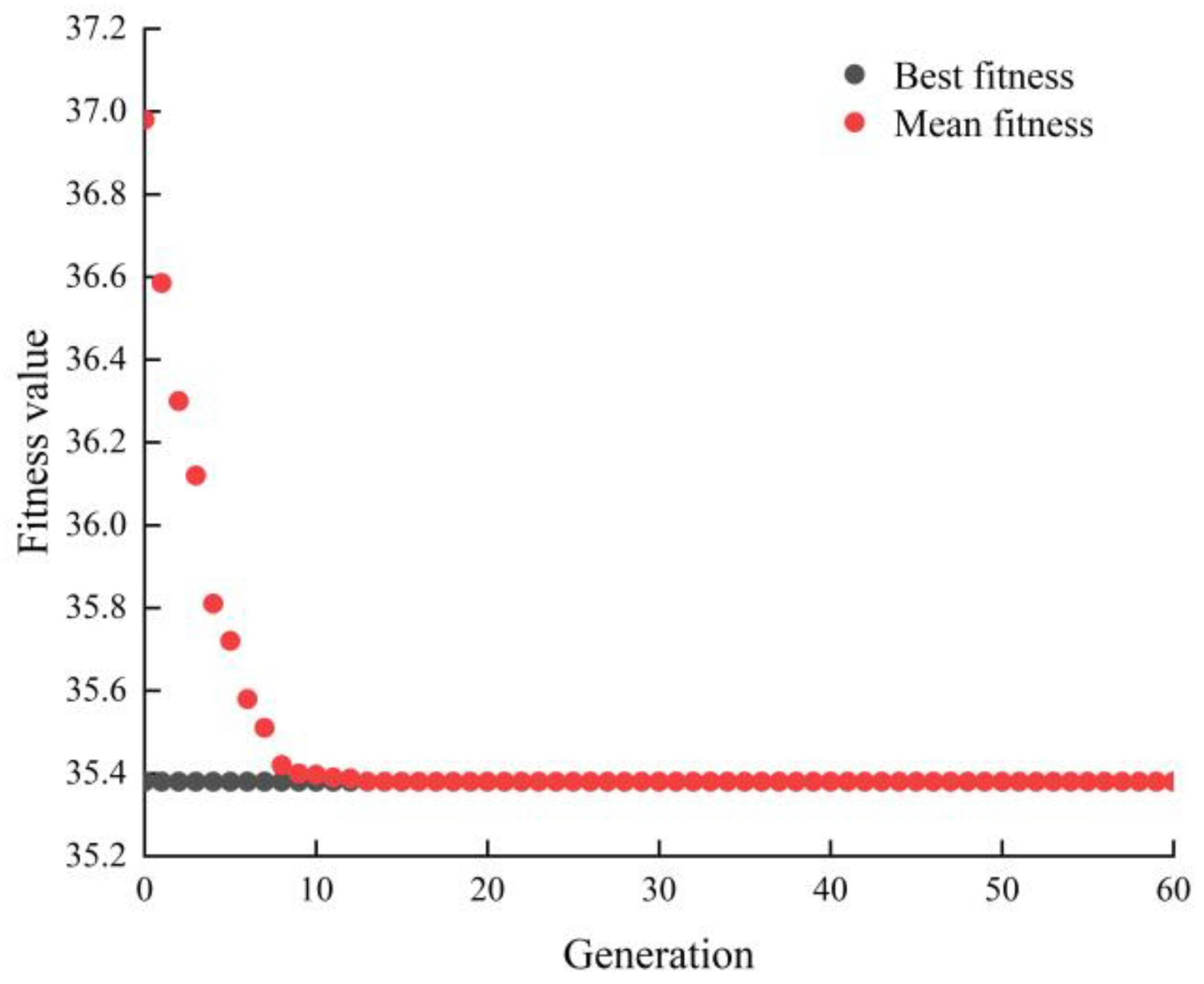
3.3. Genetic Algorithm Objective Function Solution

In order to ensure that the planned path meets the requirements, it is necessary to reasonably set the coefficients of the fifth-degree polynomial, due to the objective function is more, it is not easy to set through the empirical method, so it adopts the genetic algorithm to optimize the polynomial coefficients, which not only ensures that the planned path meets the requirements, but also ensures that the algorithm’s ability to adapt to the different working conditions, and improves the robustness of the algorithm. Figure 7 shows the results of the genetic algorithm, from which it can be seen that the genetic algorithm in the iteration to the tenth generation has been able to find the optimal solution, the time complexity is low and can be used for five polynomial parameter optimization.

3.4. Evaluation Function Design

The purpose of designing the evaluation function is to select the avoidance curve with good performance, and the evaluation function K can reflect the driving safety, comfort, and avoidance performance. In the avoidance process, the smaller the maximum longitudinal acceleration, the better the comfort of the vehicle during avoidance, and the larger the longitudinal displacement required for avoidance. The evaluation index is:

$$K={\gamma }_1{\displaystyle \frac{\sqrt{a_{\mathrm{xmax}}^2+a_{\mathrm{ymax}}^2}}{a_{\max }}}+{\gamma }_2{\displaystyle \frac{L}{{\mathrm{L}}_{\max }}}$$

(29)

In the formula, a_xmax indicates the maximum value of avoidance longitudinal acceleration, a_ymax indicates the maximum value of avoidance transverse acceleration, γ₁, γ₂ for the weight coefficients, γ₁ + γ₂ = 1, if the comfort requirements of lane changing is high, then increase the value of γ₁; if the efficiency requirements of lane changing is high, then increase the value of γ₂, the smaller the K is the better the performance of avoidance paths, according to the avoidance of the requirements of the safety and comfort of the time to adjust the value of γ₁ and γ₂.

4. Path Tracking

In this chapter, intelligent vehicle path tracking control is studied based on the theory of model predictive control, and the vehicle tracking situation is shown in Figure 8. Among many path tracking algorithms, Model Predictive Control (MPC) can carry out mathematical optimization according to the system model, and in terms of data processing, it is able to deal with complex multi-input and output problems containing constraints. In terms of data processing, it can handle complex multi-input and output problems with constraints; in terms of control performance, it is robust and easy to implement; and in the process of algorithm operation, it has the functions of prediction, feedback, and optimization [36]. MPC can predict future outputs according to the current state and inputs, and when a cycle is over, it can realize better control after feedback correction relative to the actual output.

4.1. MPC Principles

In this paper, we use approximate linearization to linearize the nonlinear system, assuming that the vehicle state equation has a working point (ξ(t), u(t)) at the moment t. The Taylor expansion is carried out at this working point, and in order to improve the computational accuracy, a first-order term can be obtained by retaining the first-order term:

$${\dot{\xi }}_d=A_d\left(t\right){\tilde{\xi }}_d\left(t\right)+B_d\left(t\right){\tilde{u}}_d\left(t\right)$$

(30)

where Ad (t) and Bd (t) are Jacobi matrices, $A_d\left(t\right)={\displaystyle \frac{\partial f\left(\delta \left(t\right),u\left(t\right)\right)}{\partial \delta }}{\mid }_{\delta \left(t\right),\mathrm{u}\left(t-1\right)}$, $B_d\left(t\right)={\displaystyle \frac{\partial f\left(\delta \left(t\right),u\left(t\right)\right)}{\partial u}}{\mid }_{\delta \left(t\right),u\left(t-1\right)}$, ${\bar{\xi }}_d\left(t\right)$ and ${\tilde{\mathrm{u}}}_d\left(t\right)$ denote the difference between the state and control quantities at moments t and t−1, and ${\tilde{\xi }}_d\left(t\right)=\xi \left(t\right)-\xi \left(t-1\right)$, ${\tilde{u}}_d\left(t\right)=u\left(t\right)-u\left(t-1\right)$.

The discretization of Equation (30) using the first-order difference quotient method yields the discrete linear time-varying system as follows:

$${\xi }_d\left(k+1\right)=A_d\left(k\right)\xi \left(t\right)+B_d\left(k\right)u\left(t\right)$$

(31)

where $A_d\left(k\right)=I+T{A}_d\left(t\right),B_d\left(k\right)=T{B}_d\left(t\right)$.

Assumptions according to Equation (30):

$$\xi \left(k,t\right)=\left[\begin{array}{c}\Delta \xi \left(k,t\right)\\ u\left(k-1,t\right)\end{array}\right]$$

(32)

By combining the system state quantities and control increments, a new state space equation can be obtained.

$$\left\{\begin{array}{l}\xi \left(k+1,t\right)={\tilde{A}}_{k,t}\xi \left(k,t\right)+{\tilde{B}}_{k,t}\Delta u\left(k,t\right)\hfill \\ \eta \left(k,t\right)=h_{k,t}\xi \left(k,t\right)\hfill \end{array}\right.$$

(33)

where $\left.{\tilde{A}}_{k,t}=\left[\begin{array}{cc}{A}_{k,t}& B_{k,t}\\ 0_{m\times n}& I_m\end{array}\right.\right],{\tilde{B}}_{k,t}=\left[\begin{array}{c}{B}_{k,t}\\ I_m\end{array}\right],{\tilde{h}}_{k,t}=\left[b_{k,t},0\right]$.

Let the prediction time domain be Np, the control time domain be Nc, and the relationship between the system state quantities and system output quantities in the prediction time domain be:

$$Y\left(t\right)={\Psi }_t\xi \left(t\right)+{\theta }_t\Delta u\left(t\right)$$

(34)

where $\left.Y\left(t\right)=\left[\begin{array}{c}\eta \left(t+1\right)\\ \eta \left(t+2\right)\\ \dots \\ \eta \left(t+N_{\mathrm{c}}\right)\\ \dots \\ \eta \left(t+N_{\mathrm{p}}\right)\end{array}\right.\right],{\Psi }_i=\left[\begin{array}{c}{C}_t{A}_t\\ C_t{A}_t^2\\ \dots \\ C_t{A}_t^{N_c}\\ \cdots \\ C_t{A}_t^{N_p}\end{array}\right],\Delta u\left(t\right)=\left[\begin{array}{c}\Delta u\left(t\right)\\ \Delta u\left(t+1\right)\\ \dots \\ \Delta u\left(t+N_c\right)\end{array}\right],$

${\theta }_t=\left[\begin{array}{cccc}{h}_t{B}_t& 0& 0& 0\\ h_t{A}_t{B}_t& h_t{B}_t& 0& 0\\ \dots & \dots & \ddots & \dots \\ h_t{A}_t^{N_c-1}{B}_t& h_t{A}_t^{N_c-2}{B}_t& \dots & h_t{B}_t\\ h_t{A}_t^{N_c}{B}_t& h_t{A}_t^{N_c-1}{B}_t& \cdots & h_t{A}_t{B}_t\\ ⋮& ⋮& \ddots & ⋮\\ h_t{A}_t^{N_p-1}{B}_t& h_t{A}_t^{N_c-2}{B}_t& \cdots & h_t{A}_t^{N_p-N_c-1}{B}_t\end{array}\right]$

4.2. Objective Function Design

In the tracking process, the deviation of the actual trajectory from the reference trajectory should be as small as possible, and the front wheel angle and angle increment should be within a certain range. In order to prevent the system from having no solution, the weight coefficient ρ and the relaxation factor ε are added into the objective function, and the objective function of the predictive control of the linear model is designed:

$$J\left({\xi }_d\left(t\right),v_d\left(t-1\right),\Delta u_d\left(t-1\right)\right)={{\displaystyle \sum }}_{i=1}^{N_{\mathrm{p}}}\parallel {\eta }_d\left(t+i|t\right)-{\eta }_{ref}\left(t+i|t\right){\parallel }_{\mathrm{Q}}^2+{{\displaystyle \sum }}_{i=1}^{N_c-1}\parallel \Delta u_d\left(t+i|t\right){\parallel }_{\mathrm{R}}^2+\rho {\epsilon }^2$$

(35)

$$\begin{array}{l}\mathrm{s}.\mathrm{t}.\hfill \\ u_{\min }\left(t+k\right)\le u\left(t+k\right)\le u_{\max }\left(t+k\right),k=0,1,\cdots ,N_c-1\hfill \\ \Delta u_{\min }\left(t+k\right)\le \Delta u\left(t+k\right)\le \Delta u_{\max }\left(t+k\right),k=0,1,\cdots ,N_c-1\hfill \\ y_{\min }\left(t+k\right)\le y\left(t+k\right)\le y_{\max }\left(t+k\right),k=0,1,\cdots ,N_c-1\hfill \end{array}$$

where Q is the error weight matrix and R is the control increment weight matrix.

4.3. Constraint Establishment

In addition to constraining the control quantities, control increments and outputs of the state equations, the parameters of the vehicle itself are constrained to ensure that the parameters do not exceed the limits of the vehicle dynamics.

(1)

Center-of-mass lateral deflection constraints.

$$\left\{\begin{array}{l}-{12}^{\circ }<\beta <{12}^{\circ }, \mathrm{good} \mathrm{road} \mathrm{surface}\hfill \\ -2^{\circ }<\beta <2^{\circ }, \mathrm{ice} \mathrm{road}\hfill \end{array}\right.$$

(36)

(2)

Pavement adhesion coefficient constraints.

$$\sqrt{a_x^2+a_y^2}\le \mu g$$

(37)

(3)

Tire side deflection constraints.

$$-2^{\circ }<{\alpha }_f<2^{\circ }$$

(38)

4.4. Simulation of Path Tracking and Result Analysis

By comparing the MPC path tracking performance under different control horizons, the impact of the control horizon on tracking performance is evaluated, and the effectiveness of the designed controller is observed. The intelligent electric vehicle is set as the controlled vehicle, and the avoidance scenario is configured on a two-lane straight road segment with a lane width of 3.75 m. The road surface adhesion coefficient is set to μ = 0.8μ = 0.8μ = 0.8, representing a good road condition. The initial speed of the avoiding vehicle is set to 17 m/s. A dynamic traffic vehicle is positioned 40 m ahead in the same lane, traveling at a speed of 18 m/s with a deceleration of 2 m/s². The left front lane is available for avoidance maneuvers. The simulation results are shown in Figure 8.

Figure 8 presents the tracking performance of the LQR and MPC controllers along a predefined path. As shown in Figure 8a, the tracking error of the LQR controller is larger than that of the MPC controller, though both controllers exhibit satisfactory tracking performance. Figure 8b indicates that the front-wheel steering angle of the MPC controller is smoother and has a smaller range compared to the LQR controller. Additionally, Figure 8c shows that the yaw rate remains nearly identical for both controllers. However, Figure 8d highlights a distinct difference in the vehicle’s sideslip angle, where the MPC controller maintains a more stable and smaller variation range than the LQR controller. These results demonstrate that for obstacle avoidance scenarios, the MPC controller outperforms the LQR controller in tracking accuracy.

In the MPC controller, key parameters include the prediction horizon Np, control horizon Nc, error weight matrix Q, and control increment weight matrix R. The control horizon Nc represents the number of optimization variables used to achieve optimal output over Np prediction steps, and it is always smaller than the prediction horizon. In this study, the prediction horizon is set to 60, while the control horizon is varied among Nc = 10, Nc = 30, and Nc = 50.

As illustrated in Figure 8a, under different control horizons, the tracking paths closely follow the target path, with minimal lateral tracking errors. Figure 8b reveals that as Nc increases, the front-wheel steering angle range expands, and the response time slightly decreases. However, beyond a certain threshold, further increases in Nc have negligible effects on system performance. Figure 8c shows minimal variation in yaw rate across different control horizons. Meanwhile, Figure 8d indicates that for Nc = 10 and Nc = 50, noticeable fluctuations in the sideslip angle occur in localized regions, whereas for Nc = 30, the sideslip angle remains more stable with a smaller variation range. Overall, Figure 8 demonstrates that the control horizon has a limited impact on tracking performance. Selecting an appropriate control horizon for a given prediction horizon can effectively reduce peak parameter values and enhance the smoothness of the obstacle avoidance process [37].

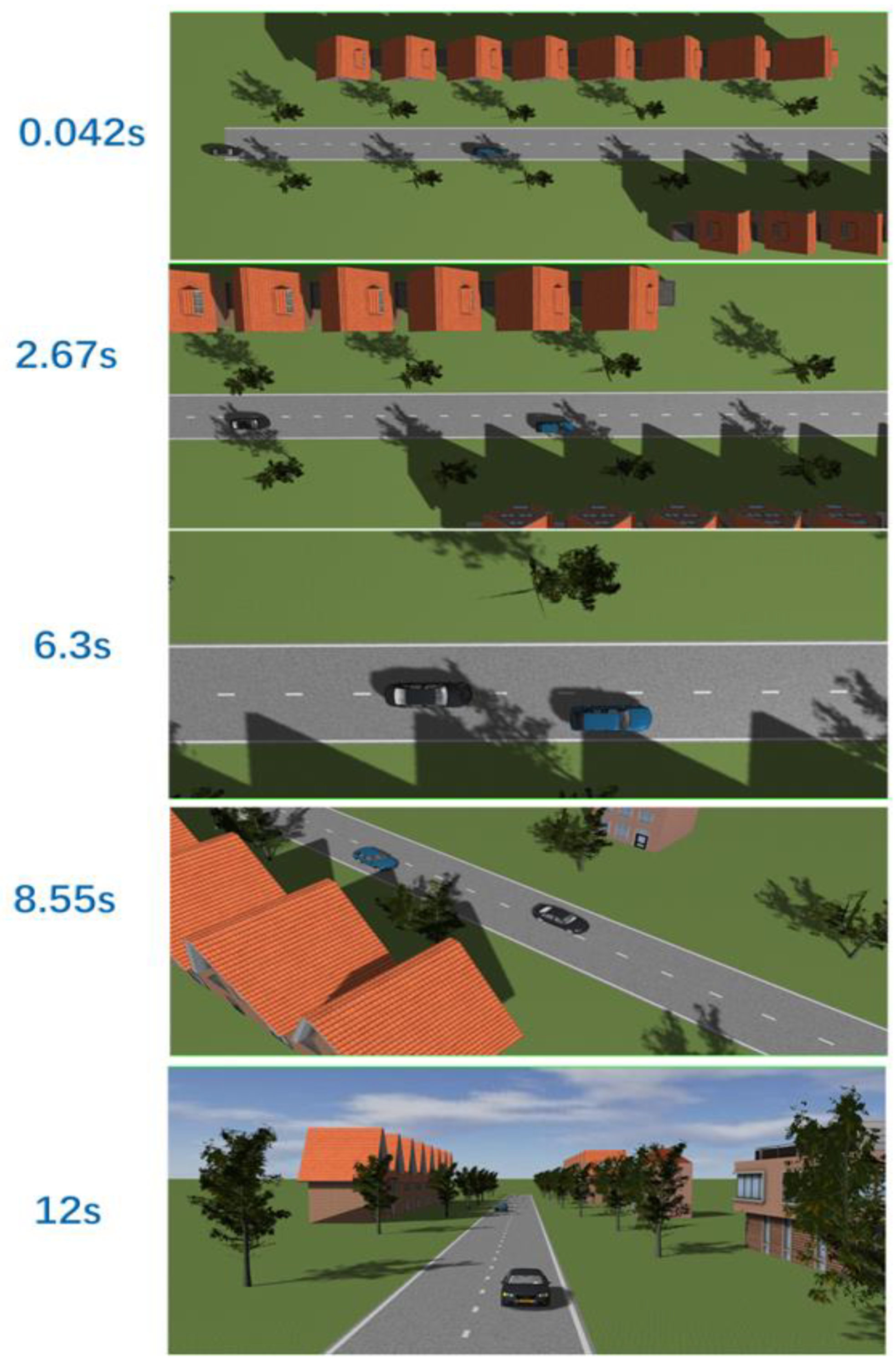
5. Simulation Verification

In order to verify the effectiveness of the proposed algorithm, this paper uses three software, Carsim 2019.0, Matlab R2023a, and Prescan 8.5.0, to carry out joint simulation and verification. These functions can assist in simulation and better simulate the real environment [38]. The relevant parameters of vehicle dynamics are set through Carsim, as shown in

Table 2. Vehicle model parameters.

Parameter	Value	Unit
Vehicle mass	1723	kg
Vehicle length	4	m
Vehicle width	1.9	m
Center of mass height	0.54	m
Front Tire Cornering Stiffness	66,900	N·rad−1
Rear Tire Cornering Stiffness	62,700	N·rad−1
Distance from front wheel to center of mass	1.232	m
Distance from the rear wheel to the center of mass	1.468	m
Moment of inertia around the z-axis	4175	Kg·m2

, the vehicle’s operating environment and sensors are set through Prescan, the model of the control algorithm is constructed through Simulink, and the vehicle information required for the algorithm is input into Simulink by Carsim and Prescan input the vehicle information required by the algorithm into Simulink, and then control the vehicle motion by solving the designed objective function and returning the control quantity to Prescan.

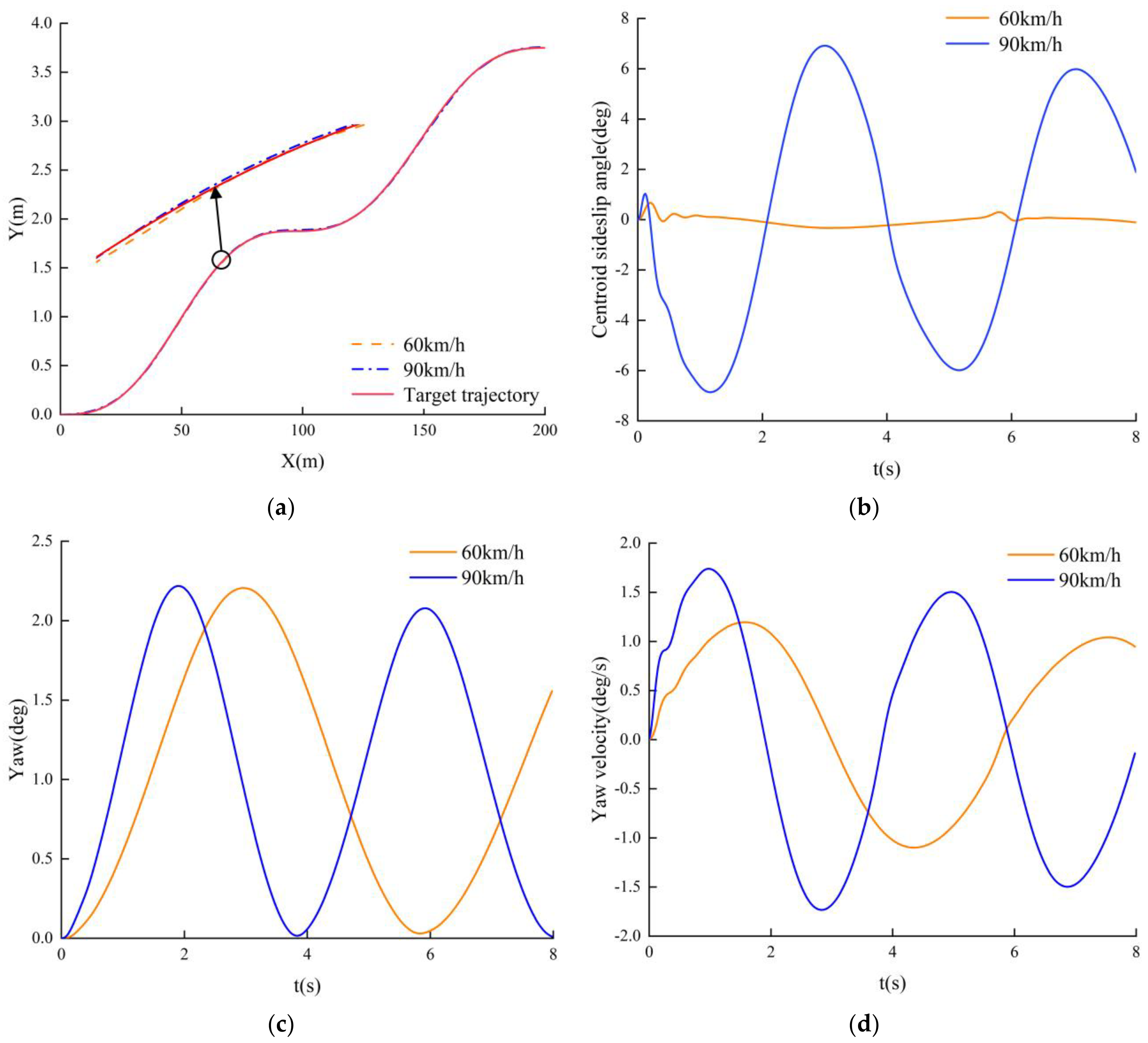
5.1. Effect of Vehicle Speed on the Controller

Avoidance scene set two lanes of straight road, with a lane width of 3.75 m, an avoidance vehicle initial speed of 60 km/h, the same lane as the car in front of the 40 m at the dynamic traffic car, traffic car deceleration, deceleration of 2 m/s², lane left in front of the ability to meet the needs of avoidance, simulation at 60 km/h and 90 km/h, respectively. The simulation results are shown in Figure 9.

Figure 9 for the active avoidance simulation effect, the figure can be seen, the vehicle from the center line of this lane, 2.67 s when the vehicle is in the first avoidance process, gradually to the lane demarcation line movement; 6.3 s when the vehicle after the first avoidance of the end of the position, the position is at the beginning of the second avoidance of the position of the vehicle to arrive at the lane demarcation line, and then the vehicle began to carry out the second lane change, which is 8.55 s when the vehicle in the second tracking process. It can be seen that the vehicle’s lateral displacement is obvious and is moving towards the target point; and at 12 s when the vehicle is close to the final target position, it can be seen that the vehicle position is in the centerline of the next lane, the end of the avoidance process.

From Figure 10a, it can be seen that the controller has good control performance at different vehicle speeds, and the speed has an effect on the vehicle path tracking control, but it is within the acceptable range; from Figure 10b, it can be seen that the center-of-mass lateral deflection angle varies within the constraints, and since the MPC is more sensitive to the speed, the greater the speed is, the more pronounced the change in the center of mass lateral deflection angle is, and then a larger control amount is needed to compensate for the tracking error; in Figure 10c,d, it can be seen that the higher the speed, the faster the Yaw angle and yaw velocity response. In summary, at different speeds under the action of the controller, the vehicle can follow the expected tracking path to ensure the stability of vehicle driving, reflecting the robustness of the controller [39].

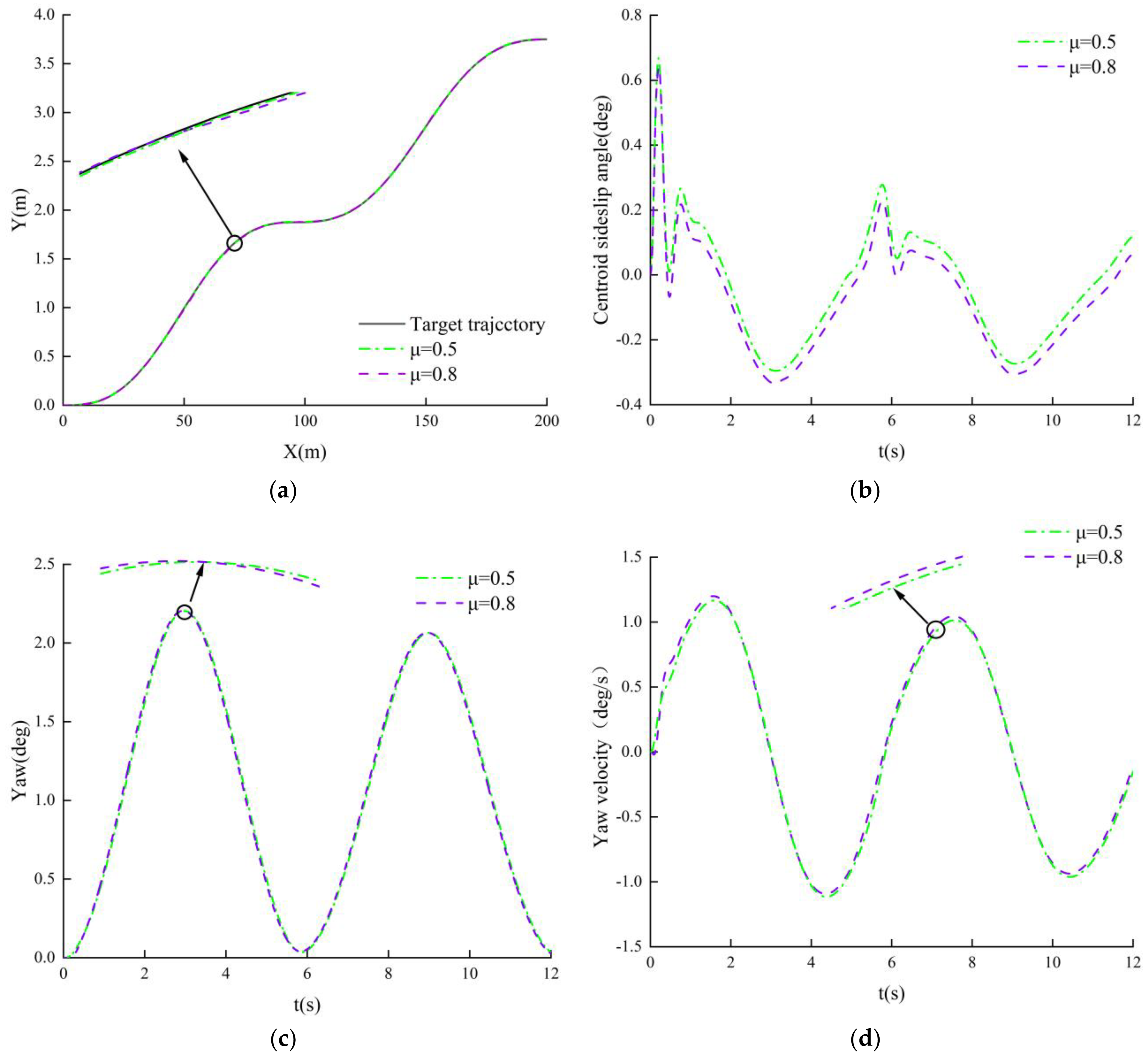
5.2. Influence of the Road Surface Adhesion Coefficient on the Controller

Keeping the other parameter settings unchanged, change the pavement adhesion coefficient, set μ = 0.8 for good pavement and μ = 0.5 for slippery pavement, and continue to carry out the simulation. The simulation results are shown in Figure 11.

According to Figure 11a, the vehicle can smoothly complete the avoidance operation under two different road surfaces, and the tracking ability of the path is good, with a maximum error of 0.002 m. According to Figure 11b–d, it can be seen that the controller has a good tracking stability performance in environments with a vehicle speed of 60 km/h, and different road adhesion coefficients; wherein, the center of mass lateral deflection angle, the yaw angle, the changes in yaw angle and speed are all within the constraint control range. In summary, the control system can track the preset path stably under μ = 0.5 and μ = 0.8 road conditions, with good control performance [40].

6. Conclusions

This paper researches the active avoidance path planning and tracking control problem of intelligent vehicles, and proposes a new path planning and tracking control method with the following conclusions:

(1)

The scheme is feasible to control the active avoidance of intelligent vehicles using hierarchical control.

(2)

The double quintic polynomial avoidance algorithm designed by integrating a genetic algorithm converts the avoidance path planning problem into a nonlinear planning problem and solves the optimal avoidance path by genetic algorithm under the satisfaction of boundary conditions as well as constraints. Simulation results show that the designed avoidance algorithm has high real-time and robustness.

(3)

An MPC path tracking controller is designed based on intelligent vehicles and a predefined path. The objective function and controller constraints are formulated according to the dynamic requirements of intelligent vehicles, while the preview step size and sampling period in MPC are adjusted in real time. Simulation results demonstrate that the trajectory tracking controller improves tracking accuracy while ensuring vehicle stability [41]. Moreover, it exhibits good adaptability and stability under varying vehicle speeds and road adhesion conditions.

Although the combination of the quintic polynomial and genetic algorithm enhances the adaptability of path planning, the iterative optimization process of the genetic algorithm incurs a high computational load, potentially compromising real-time performance. Moreover, the current hierarchical approach does not account for obstacle avoidance triggering conditions or multi-objective conflict resolution, which may lead to suboptimal performance in complex traffic scenarios.

In this paper, only the path planning and tracking control algorithm is studied, and no avoidance judgment strategy is added, and the future will continue to study the avoidance strategy selection. The designed avoidance scenarios include certain idealized assumptions, and the traffic participants involved in the avoidance process are not sufficiently complex. Future work can expand the scenarios and develop more effective strategies to enhance applicability. Due to the limitation of hardware conditions, only simulation tests are carried out in the paper, real-vehicle testing has not yet been conducted, making it impossible to fully validate the reliability of the algorithm in real-world traffic environments, and the algorithm has not been applied to the real vehicle to verify the algorithm, and the algorithm’s effect on the real vehicle can be further tested in the future.

References

1. An, L.; Chen, T.; Cheng, A.; Fang, W. A simulation on the path planning of intelligent vehicles based on artificial potential field algorithm. Automot. Eng. 2017, 39, 1451–1456. [Google Scholar]
2. Hu, Y.; Qu, T.; Liu, J.; Shi, Z.Q.; Zhu, B.; Cao, D.P.; Chen, H. Human-machine cooperative control of intelligent vehicle: Recent developments and future perspectives. Acta Autom. Sin. 2019, 45, 1261–1280. [Google Scholar]
3. Zha, Y.; Yu, M.; Ma, F.; Zheng, X. Research on path tracking for intelligent driving vehicle based on steering-by-wire. Automob. Technol. 2021, 7–13. [Google Scholar] [CrossRef]
4. Wei, T.; Chen, L. Path planning for mobile robot based on improved genetic algorithm. J. Beijing Univ. Aeronaut. Astronaut. 2020, 46, 703–711. [Google Scholar]
5. Zheng, H.; Feng, G.; Pu, W.; Xu, M. Global Path Planning in a Closed Environment Based on the DijkstraAlgorithm. Automot. Pract. Technol. 2023, 48, 7–11. [Google Scholar] [CrossRef]
6. Ren, B.; Wang, X.; Deng, W.; Nan, J.; Zong, R.; Ding, J. Path optimization algorithm for automatic parking based on hybrid A* and reeds-shepp curve with variable radius. China J. Highw. Transp. 2022, 35, 317–327. [Google Scholar]
7. Ren, X. Research on Path Planning of Self-Driving Vehicle Based on Improved RRT Algorithm. Master’s Thesis, Chang’an University, Xi’an, China, 2021. [Google Scholar]
8. Yu, Z.; Li, Y.; Xiong, L. A Review of Motion Planning Algorithms for Autonomous Vehicles. J. Tongji Univ. (Nat. Sci. Ed.) 2017, 45, 1150–1159. [Google Scholar]
9. Zhou, W.; Guo, X.; Pei, X.; Zhang, Z.; Yu, J. Study on path planning and tracking control for intelligent vehicle based on RRT and MPC. Automot. Eng. 2020, 42, 1151–1158. [Google Scholar]
10. Du, M.; Mei, T.; Chen, J.; Zhao, P.; Liang, H.; Huang, R.; Tao, X. RRT-based motion planning algorithm for intelligent vehicle in complex environments. Robot 2015, 37, 443–450. [Google Scholar]
11. Arab, A.; Yu, K.; Yi, J.; Song, D. Motion planning for aggressive autonomous vehicle maneuvers. In Proceedings of the 2016 IEEE International Conference on Automation Science and Engineering (CASE), Fort Worth, TX, USA, 21–25 August 2016; IEEE: Piscataway, NJ, USA, 2016; pp. 221–226. [Google Scholar]
12. Li, X.; An, H. Research on Path Planning for Unmanned Delivery Vehicles Based on Genetic Algorithm. Logist. Technol. 2024, 47, 4–7. [Google Scholar] [CrossRef]
13. Li, Z.; Jia, Y.; Jiang, X. Research on Mobile Robot Path Planning Based on Improved Genetic Algorithm. Mod. Inf. Technol. 2024, 8, 180–183+188. [Google Scholar] [CrossRef]
14. Wang, X.; Shi, H.; Zhang, C. Path planning for intelligent parking system based on improved ant colony optimization. IEEE Access 2020, 8, 65267–65273. [Google Scholar] [CrossRef]
15. Han, G.; Fu, W.; Wang, W. The study of intelligent vehicle navigation path based on behavior coordination of particle swarm. Comput. Intell. Neurosci. 2016, 2016, 6540807–6540817. [Google Scholar] [CrossRef]
16. Li, H.; Luo, Y.; Wu, J. Collision-free path planning for intelligent vehicles based on Bézier curve. IEEE Access 2019, 7, 123334–123340. [Google Scholar] [CrossRef]
17. Ghariblu, H.; Moghaddam, H.B. Trajectory planning of autonomous vehicle in freeway driving. Transp. Telecommun. J. 2021, 22, 278–286. [Google Scholar] [CrossRef]
18. Chen, L.; Qin, D.; Xu, X.; Cai, Y.; Xie, J. A path and velocity planning method for lane changing collision avoidance of intelligent vehicle based on cubic 3-D Bezier curve. Adv. Eng. Softw. 2019, 132, 65–73. [Google Scholar] [CrossRef]
19. Niu, G.; Li, W.; Wei, H. Intelligent vehicle lane changing trajectory planning based on double quintic polynomials. Automot. Eng. 2021, 43, 978–986+1004. [Google Scholar]
20. Sun, Y. Quantitative Evaluation of Intelligence Levels for Unmanned Ground Vehicles. Master’s Thesis, Beijing Institute of Technology, Beijing, China, 2014. [Google Scholar]
21. Yao, Q.; Tian, Y.; Wang, Q.; Wang, S. Control Strategies on Path Tracking for Autonomous Vehicle: State of the Art and Future Challenges. IEEE Access 2020, 8, 161211–161222. [Google Scholar] [CrossRef]
22. Carlucho, I.; De Paula, M.; Acosta, G.G. An adaptive deep reinforcement learning approach for MIMO PID control of mobile robots. ISA Trans. 2020, 102, 280–294. [Google Scholar] [CrossRef]
23. Nie, X.; Xiong, Y.; Pan, Y. Multi-condition co-simulations of vehicle stability control via fuzzy pid algorithm. J. Dyn. Control 2021, 19, 46–52. [Google Scholar]
24. Wang, X.; Ling, M.; Rao, Q.; Liu, C.; Zhai, S. Research on fusion algorithm of unmanned vehicle path tracking based on improved stanley algorithm. Automob. Technol. 2022, 7, 25–31. [Google Scholar]
25. Amer, N.H.; Hudha, K.; Zamzuri, H.; Aparow, V.R.; Abidin, A.F.Z.; Kadir, Z.A.; Murrad, M. Adaptive modified Stanley controller with fuzzy supervisory system for trajectory tracking of an autonomous armoured vehicle. Robot. Auton. Syst. 2018, 105, 94–111. [Google Scholar] [CrossRef]
26. Sun, Y.; Dai, Q.; Liu, J.; Zhao, X.; Guo, H. Intelligent vehicle path tracking based on feedback linearization and LOR under extreme conditions. In Proceedings of the 2022 41st Chinese Control Conference (CCC), Hefei, China, 25–27 July 2022; pp. 5383–5389. [Google Scholar]
27. Zhang, J.; Yang, M.; Chen, Y.D.; Li, H.; Chen, N.; Zhang, Y. Research on Sliding Mode Control for Path Following in Variable Speed of Unmanned Vehicles. Optim. Eng. 2025, 1–28. [Google Scholar] [CrossRef]
28. Xie, X.; Wang, Y.; Jin, L.; Guo, B.; Wei, Q.; He, Y. MPC Trajectory Tracking Control Based on Changing Control Time-Step Length. J. Jilin Univ. (Eng. Ed.) 2022, 1–10. [Google Scholar] [CrossRef]
29. Guirguis, J.M.; Hammad, S.; Maged, S.A. Path tracking control based on an adaptive MPC to changing vehicle dynamics. Int. J. Mech. Eng. Robot. Res. 2022, 11, 535–541. [Google Scholar] [CrossRef]
30. Wang, Y.; Cai, Y.; Chen, L.; Wang, H.; Li, J.; Chu, X. Design of a Path Tracking Controller for Intelligent Vehicles Based on Model Predictive Control. Automot. Technol. 2017, 10, 44–48. [Google Scholar] [CrossRef]
31. Li, S.; Zhang, M. Research on Lane Change Path Planning for Intelligent Vehicles Based on Dual Quintic Polynomials. J. Nanjing Univ. Inf. Sci. Technol. 2024, 16, 155–163. [Google Scholar] [CrossRef]
32. Zhang, P.; Chen, Y.; Jiang, S.; Han, Y. Trajectory Planning and Tracking Control for Autonomous Overtaking on Highways. J. Automot. Saf. Energy 2022, 13, 463–472. [Google Scholar]
33. Liang, C.; Li, Y.; Li, Z.; Shen, Z. Dynamic Performance Research of the Magic Formula Tire Model. Automot. Pract. Technol. 2020, 45, 116–119. [Google Scholar] [CrossRef]
34. Gong, J.; Jiang, Y.; Xu, W. Model Predictive Control for Self-Driving Vehicles; Beijing Institute of Technology Press: Beijing, China, 2014. [Google Scholar]
35. Nam, H.; Choi, W.; Ahn, C. Model predictive control for evasive steering of an autonomous vehicle. Int. J. Automot. Technol. 2019, 20, 1033–1042. [Google Scholar] [CrossRef]
36. Li, G. Vehicle Obstacle Avoidance Path Planning and Tracking Based on Model Predictive Control. Automot. Pract. Technol. 2024, 49, 49–54. [Google Scholar] [CrossRef]
37. Gu, X.; Li, J. Path Tracking Control Method for Autonomous Vehicles. Automot. Eng. 2019, 264, 11–14. [Google Scholar]
38. Lu, Y. Study on PreScan/CarSim/Simulink Combined Simulation Method. J. Jiamusi Univ. (Nat. Sci. Ed.) 2020, 38, 118–121. [Google Scholar]
39. Zhu, B.; Zhang, P.; Liu, B.; Zhao, J.; Sun, Y. Safety Evaluation Method for Autonomous Vehicles Based on Natural Driving Data. China J. Highw. Transp. 2022, 35, 283–291. [Google Scholar]
40. Zhang, L.; Liu, M.; Liu, Z.; Xie, L. Joint Simulation Study of Vehicle Adaptive Cruise Control System. Mech. Des. Manuf. 2022, 69–72+77. [Google Scholar] [CrossRef]
41. Du, R.; Hu, H.; Gao, K.; Huang, H. Research on Trajectory Tracking Control for Autonomous Vehicles Based on Variable Prediction Horizon MPC. J. Mech. Eng. 2022, 58, 275–288. [Google Scholar]
Figure 1. Intelligent vehicle active avoidance hierarchical control architecture.
Wevj 16 00211 g001
Figure 2. Three-degree-of-freedom monorail vehicle model.
Wevj 16 00211 g002
Figure 3. Tire longitudinal force versus slip rate curves.
Wevj 16 00211 g003
Figure 4. Curve of tire lateral force versus lateral deflection angle.
Wevj 16 00211 g004
Figure 5. Schematic diagram of active avoidance.
Wevj 16 00211 g005
Figure 6. Avoidance trajectory flowchart.
Wevj 16 00211 g006
Figure 7. Genetic algorithm calculation results.
Wevj 16 00211 g007
Figure 8. Simulation results of controller performance. (a) Path tracing. (b). Front wheel corner. (c) Yaw angle. (d) Centroid side declination.
Wevj 16 00211 g008
Figure 9. Active avoidance simulation effect.
Wevj 16 00211 g009
Figure 10. Active avoidance simulation effect. (a) Path tracing; (b) center of mass lateral deflection angle; (c) yaw angle; and (d) yaw velocity.
Wevj 16 00211 g010
Figure 11. Effect of different road surface adhesion coefficients on the controller. (a) Path tracing; (b) center of mass lateral deflection angle; (c) yaw angle; and (d) yaw velocity.
Wevj 16 00211 g011