Stochastic Optimal Scheduling of Flexible Traction Power Supply System for Heavy Haul Railway Considering the Online Degradation of Energy Storage

Abstract

The heavy-haul flexible traction power supply system (HFTPSS), integrated with an energy storage system (ESS) and power flow controller (PFC), offers significant potential for improving energy efficiency and reducing costs. However, the state of ESS capacity and the uncertainty of traction power significantly affect HFTPSS operation, creating challenges in fully utilizing flexibility to achieve economic system operation. To address this challenge, a classical scenario generation approach combining long short-term memory (LSTM), Latin hypercube sampling (LHS), and fuzzy c-means (FCM) is proposed to quantitatively characterize traction power uncertainty. Based on the generated scenarios, and considering the energy balance and safe operation constraints of HFTPSS, a stochastic optimal energy dispatch model is developed. The model aims to minimize the operational cost for heavy-haul electrified railways (HERs) while accounting for the impact of online ESS capacity degradation on the energy scheduling process. Finally, the effectiveness of the proposed strategy and model is validated using operational data from a real HER system.

1. Introduction

HERs are extensively utilized for freight transportation owing to their high load capacity and extended length. According to the International Energy Agency [1], over 66% of global freight is projected to be transported by rail in 2050. With the continuous growth in mileage and carrying capacity of heavy haul railways, energy consumption has emerged as a critical issue. In China, heavy haul railways are extensively distributed, traversing unique topography that rises in the west and slopes downward toward the east [2]. Fully loaded heavy trains operating on long, steep downhill sections generate a large amount of regenerative braking energy (RBE). However, the segmented power supply structure and traffic organization of conventional traction power supply systems result in most RBE being returned to the grid, with only a small proportion utilized by other locomotives in the same power supply area [3,4]. Therefore, enhancing RBE utilization is essential to reducing energy consumption and operational costs in heavy haul railways [5].

The traction power supply system (TPSS) integrated with ESS is regarded as the next-generation rail power system pattern [6,7], enabling efficient control of power flow among the grid, trains, and ESS [8]. TPSS is transitioning from a passive network to a bidirectional active network, providing significant economic and stability advantages. Developing an optimal operational strategy based on predictive information remains a major challenge during the day-ahead operational period. Reference [9] proposed an optimization framework for TPSS aimed at minimizing both investment and operational costs. An energy management model for ESS was introduced in [10], and reference [11] proposed a model predictive control approach for TPSS using a hierarchical structure. Existing literature focuses on energy management approaches for TPSS, yet several critical challenges remain unresolved. First, the majority of existing approaches are based on deterministic optimization, which overlooks the inherent uncertainties in traction power. Addressing these uncertainties within the optimization framework for energy management is a key challenge [12]. Furthermore, although ESS is widely acknowledged for its substantial energy-saving potential, its high installation cost necessitates the consideration of strategies to extend its operational lifetime during scheduling decisions [13].

Traditionally, the prediction of traction power flow has been addressed in certain standards [14], where a theoretical control approach simulating the interaction between trains and the railway power system, based on maximum acceleration and braking, is utilized. This method was initially developed to verify system stability rather than to achieve economic dispatch. In recent years, researchers have proposed various approaches for power prediction, which can be broadly categorized into two types: traditional statistical methods [15,16] and machine learning-based methods [17,18]. Traditional statistical forecasting techniques demonstrate superior performance when applied to periodic and smooth time series data. For instance, a fuzzy linear regression method is employed in [19] to forecast power, while Ref. [20] introduces a functional time series forecasting method to predict electricity demand and price. However, these traditional methods face challenges in accurately predicting highly random and volatile time series data. To address these limitations, machine learning methods have been increasingly adopted for load forecasting. For example, Ref. [21] employs a deep learning-based approach to forecast traction power, and Ref. [22] proposes an improved BP neural network for short-term gas power forecasting. Despite these advancements, further research is required to reduce the impact of prediction errors on system scheduling.

Addressing uncertainty-related problems is a critical aspect of railway energy management, and for this reason, robust optimization has been widely adopted [23,24,25]. For instance, a robust optimization method is proposed in [26] to address the uncertainties associated with renewable energy generation and loads. Similarly, Ref. [27] introduces a two-stage robust-stochastic model to coordinate the operations of the railway system and the power grid. However, the robust optimization approach often results in overly conservative optimization outcomes, requiring the system operator to prioritize system reliability at the expense of higher operational costs. In reality, the extreme cost contingency events considered in robust optimization are rare and can be managed within an acceptable confidence level, which highlights the effectiveness of stochastic optimization [28]. For example, Ref. [29] proposes a multi-scenario stochastic programming model to optimize the operation of an integrated energy system, while Ref. [30] presents a stochastic energy management approach for electrical railway systems. Despite the potential of stochastic optimization, clustering classical scenarios from an extensive set of possible scenarios remains a significant challenge [29].

To bridge the above gaps, this paper proposes a stochastic optimal scheduling approach for HFTPSS that accounts for the uncertainty of traction power and the online degradation of ESS, with the objective of minimizing system operation costs. The main contributions of this article are as follows:

(1)

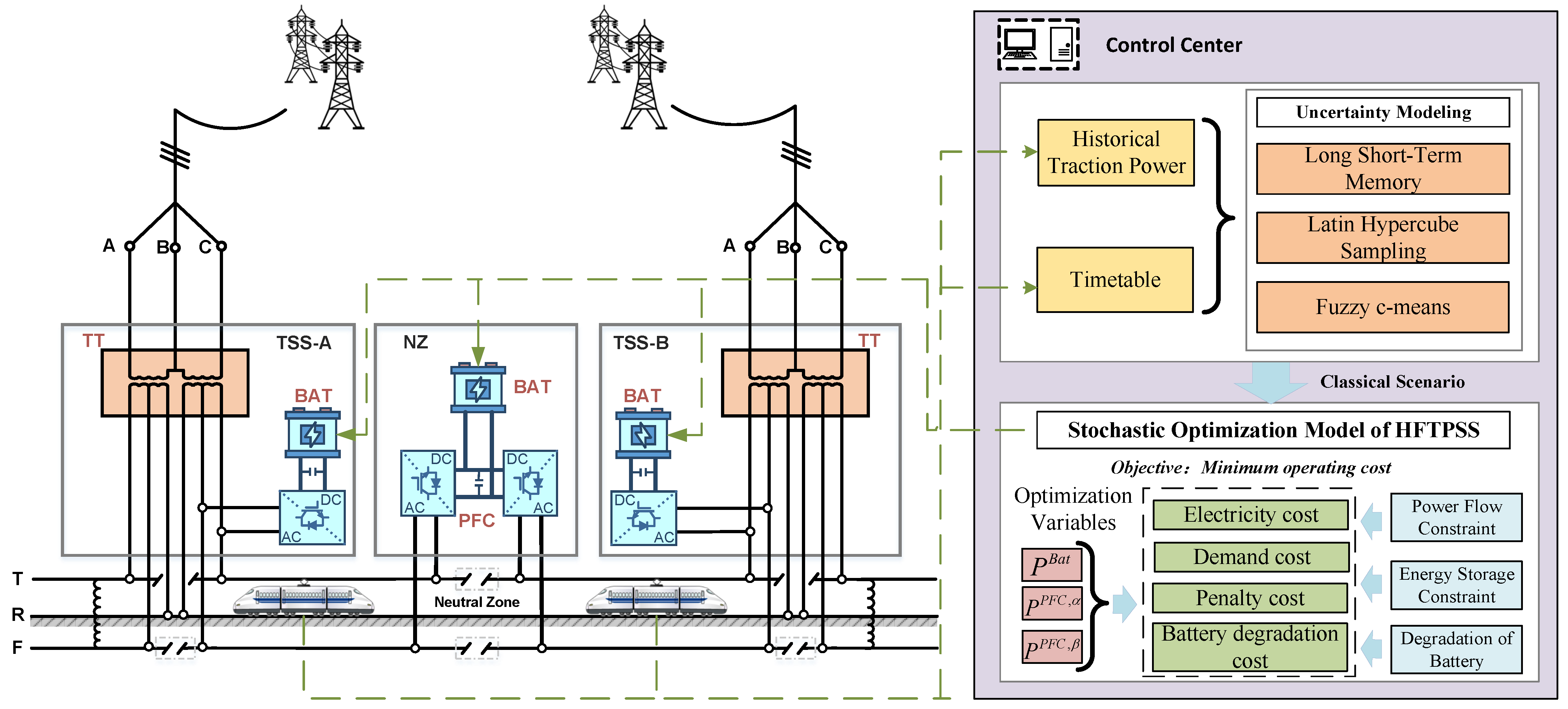
An HFTPSS integrated with ESS and PFC is developed to enhance the economic operation of the system. The PFC facilitates power interactions between various traction substations to improve the entire system’s energy efficiency, while the ESS achieves peak shaving by flexibly regulating RBE, thereby reducing the electricity costs of HFTPSS.

(2)

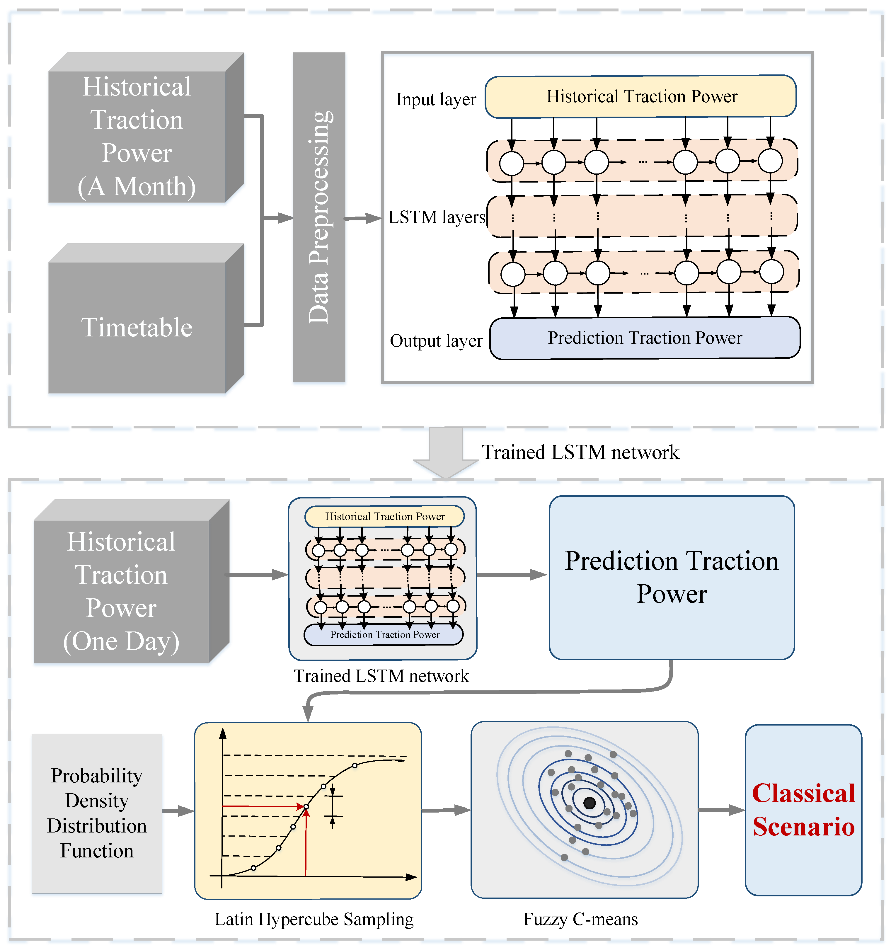
Considering the volatility of traction power in heavy-haul railways, a classical scenario generation method combining LSTM, LHS, and FCM is proposed to generate classical scenarios that reflect actual situations, accurately accounting for power uncertainty and thereby reducing its impact on system scheduling.

(3)

Taking into account the impact of traction power uncertainty and the state of ESS capacity on energy dispatch, a stochastic optimal scheduling model for HFTPSS is proposed. This model considers the online degradation of ESS and aims to improve RBE utilization, enhance energy efficiency, and reduce electricity costs by optimizing the operational strategy of flexible devices.

The rest of this paper is organized as follows: Section 2 introduces the structure of HFTPSS. Section 3 establishes the model of power uncertainty. Section 4 presents the HFTPSS optimization model, which considers battery online degradation and power uncertainty. Section 5 conducts the case study. Finally, Section 6 provides the conclusion.

2. System Description

HERs are efficient, cost-effective, and capable of handling large capacities, making them one of the key development directions for railroads in recent years. Unlike conventional freight and passenger railways, HERs are characterized by long periods of continuous traction or braking, resulting in high energy consumption and abundant RBE. However, the random departure intervals and operational states of HERs make it difficult for a significant portion of RBE to be utilized by traction trains. Consequently, this RBE is often returned to the grid, leading to substantial energy waste and high penalty costs. To enhance the economic and efficient operation of HERs, this paper proposes an HFTPSS topology, which extends the traditional TPSS by integrating PFC, composed of power electronic devices, along with an energy storage system, as illustrated in Figure 1. The system consists of two traction transformers (TT), three ESS, and one PFC. The TT step down voltage from 110 kV or 220 kV to 27.5 kV for train operations. The PFC eliminates energy barriers caused by partitioning between neighboring traction substations, enabling energy interoperability and enhancing system energy efficiency. The ESS installed in the traction substations (TSS) and neutral zones (NZ) enable flexible energy adjustment through dynamic charging and discharging, smoothing energy peaks and valleys in the HFTPSS. This improves RBE utilization and promotes the economic and low-carbon operation of the system.

However, in the energy scheduling process of HFTPSS, the uncertainty in locomotive current consumption, arising from factors such as driver behavior and environmental conditions, affects the ability of the system to regulate energy effectively. To address this, a classical scenario generation approach combining LSTM, LHS, and FCM is proposed to characterize traction power uncertainty. Based on the generated scenarios, a stochastic optimal scheduling strategy for the HFTPSS is developed, taking into account the online degradation of the battery. The objective is to minimize the combined cost of the HFTPSS, including battery degradation costs, under the classical scenarios. Finally, the charging and discharging strategy for the ESS and the control strategy for the PFC are determined.

3. Uncertainty Modeling of Traction Power

The randomness of the departure interval and the status of the train in HERs lead to high volatility of the traction power and a large amount of RBE is wasted. In order to obtain the classical scenario that reflect the power characteristic. In this section, a classical scenario generation approach integrating LSTM, LHS and FCM is proposed.

3.1. Framework of Uncertainty Modeling

Considering the error between the actual traction power with the forecast traction power [31], the traction power in the generated scenario can be expressed by the following formula, including the power forecast value and the forecast error:

$$P_{t,s}^{Load}=P_{t,pre}^{Load}+\mathrm{\Delta }{P}_{t,s}^{Load},t\in \left[1,T\right]$$

(1)

where $P_{t,s}^{Load}$ is the value of each generated scenario at time t. $P_{t,pre}^{Load}$ is the predicted value at time t. $\mathrm{\Delta }{P}_{t,s}^{Load}$ is the forecast error at time t.

According to the central limit theory, the forecast error of traction power can be expressed by a Gaussian distribution [32], the probability density function as:

$$F_t\left(\mathrm{\Delta }{P}_t^{Load}\right)={\displaystyle \frac{1}{\sqrt{2\pi }\sigma }}{e}^{-{\displaystyle \frac{{(\mathrm{\Delta }{P}_t^{Load}-\mu )}^2}{2{\sigma }^2}}},t\in \left[1,T\right]$$

(2)

where $F_t$ is the probability density function, it represents the probability of different prediction errors. $\mu$ is the expectation of the prediction error. $\sigma$ is the standard deviation of prediction errors.

The framework of uncertainty modeling is shown in Figure 2. In the first stage, input historical data to train the LSTM network. The trained network is finally obtained. At the next stage, short-term prediction uses trained neural networks. Consider the prediction error to satisfy the normal distribution function, generating the scenario set based on LHS. FCM is used for reduction until the desired number is achieved.

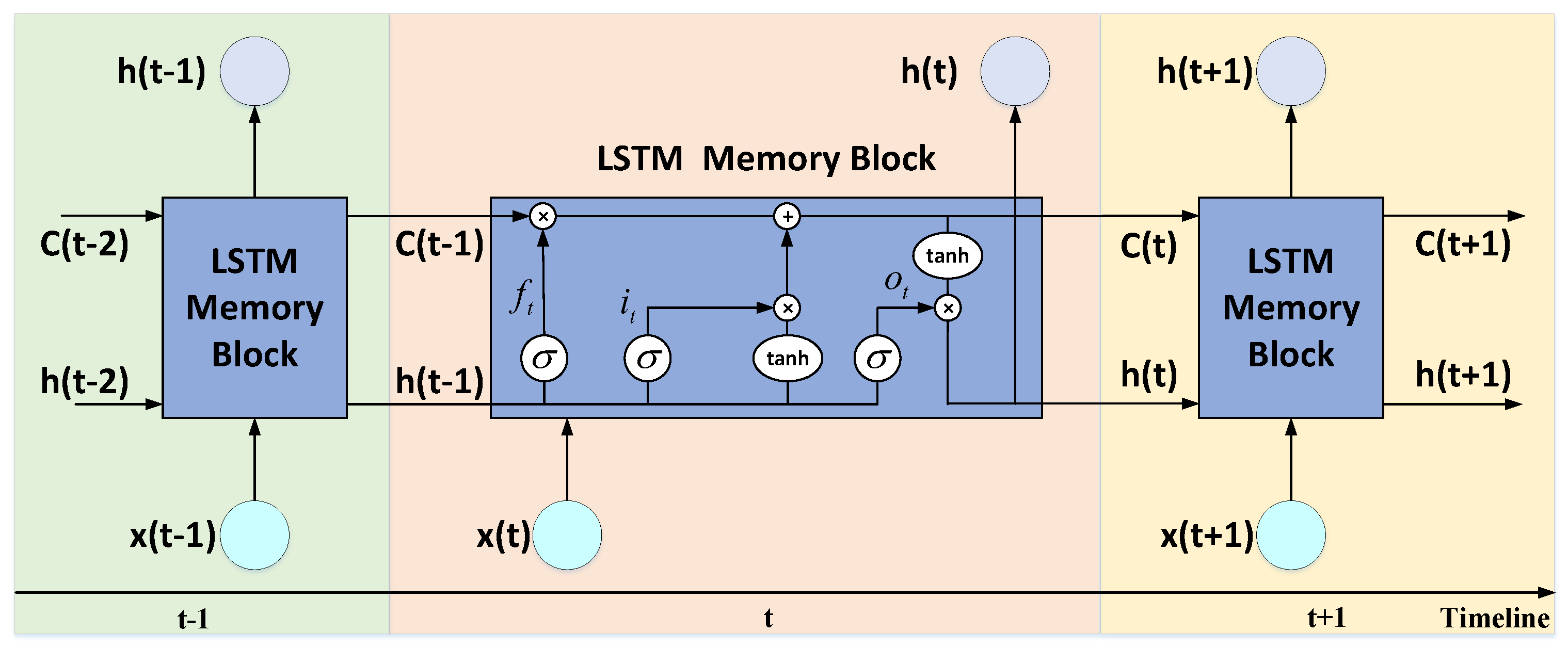
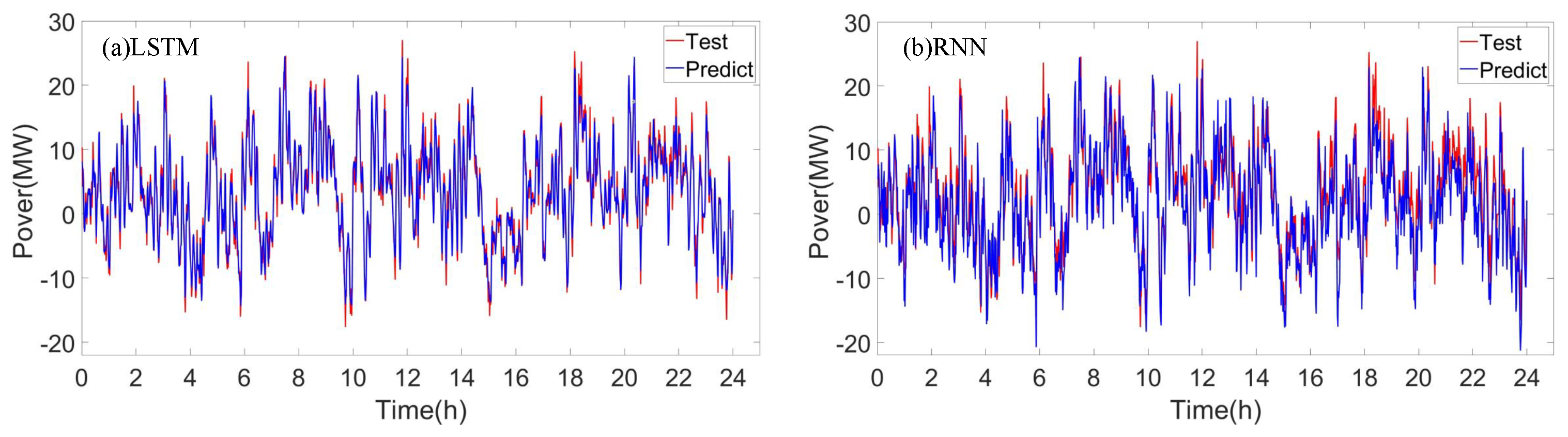
3.2. Prediction Model of Traction Power

Forecasting based on LSTM requires an input vector to be provided to the model for predicting the output [33]. In this paper, the historical data of Z time steps is used as the input feature vector, and then the output is the predicted value for one future time step. After each round of prediction, the inputs and outputs of the network model based on the LSTM window are shifted one step forward. The output window size is the total time step in the future day. In this way, the predicted value of the traction power for the coming day is obtained. The predicted value at time t can be expressed as:

$$P_{t,pre}^{Load}=f_{pre}^{LSTM}\left(\overrightarrow{{\mathbb{C}}_t}\right),t\in [1,T]$$

(3)

where $f_{pre}^{LSTM}$ denotes the relationship between the input and output of the prediction network. $\overrightarrow{{\mathbb{C}}_t}$ is the input vector at time t, $\overrightarrow{{\mathbb{C}}_t}=\left\{P_{t-Z}^{Load},P_{t-Z+1}^{Load},···,P_{t-2}^{Load},P_{t-1}^{Load}\right\}$.

LSTM is a special kind of recurrent neural network (RNN). Compared with RNN, LSTM introduces input gates, forgetting, output gates, and a cell state [34,35]. The memory of LSTM makes it able to predict the time-series data, such as the traction power well, which further improves the prediction accuracy. The structure of LSTM is shown in Figure 3. $P_{t,pre}^{Load}$ is the predicted value of traction load at time t. The calculation method of the three gates is as follows:

$$f_t=\sigma (W_{fh}·h_{t-1}+W_{fx}·x_t+b_f)$$

(4)

$$i_t=\sigma (W_{ih}·h_{t-1}+W_{ix}·x_t+b_i)$$

(5)

$$o_t=\sigma (W_{oh}·h_{t-1}+W_{ox}·x_t+b_o)$$

(6)

where $\sigma$ denotes the logic function, $h_{t-1}$ is the hidden state of the previous moment, and $x_t$ denotes the input of the moment, $W_{fh},W_{fx},W_{ih},W_{ix},W_{oh},W_{ox}$ is the weight matrices, $b_f,b_i,b_o$ is the stands for bias vectors.

At each moment, the inputs of the LSTM include the input $x_t$ of the moment t, the hidden state $h_{t-1}$ of the previous moment, and the state of the storage unit $c_{t-1}$. The outputs include the hidden state $h_t$ and the state of the unit $c_t$, and their expressions are as follows:

$$\widetilde{C_t}=tanh(W_{Ch}·h_{t-1}+W_{Cx}·x_t+b_C)$$

(7)

$$C_t=f_t·C_{t-1}+i_t·\widetilde{C_t}$$

(8)

$$h_t=o_t·tanh\left(C_t\right)$$

(9)

where $\widetilde{C\left(t\right)}$ is the updated cell state. $C\left(t\right)$ is the cell state. tanh is the tangent function. $W_{Ch},W_{Cx}$ is the weight matrices. $b_f,b_i,b_o$ is the stands for bias vectors.

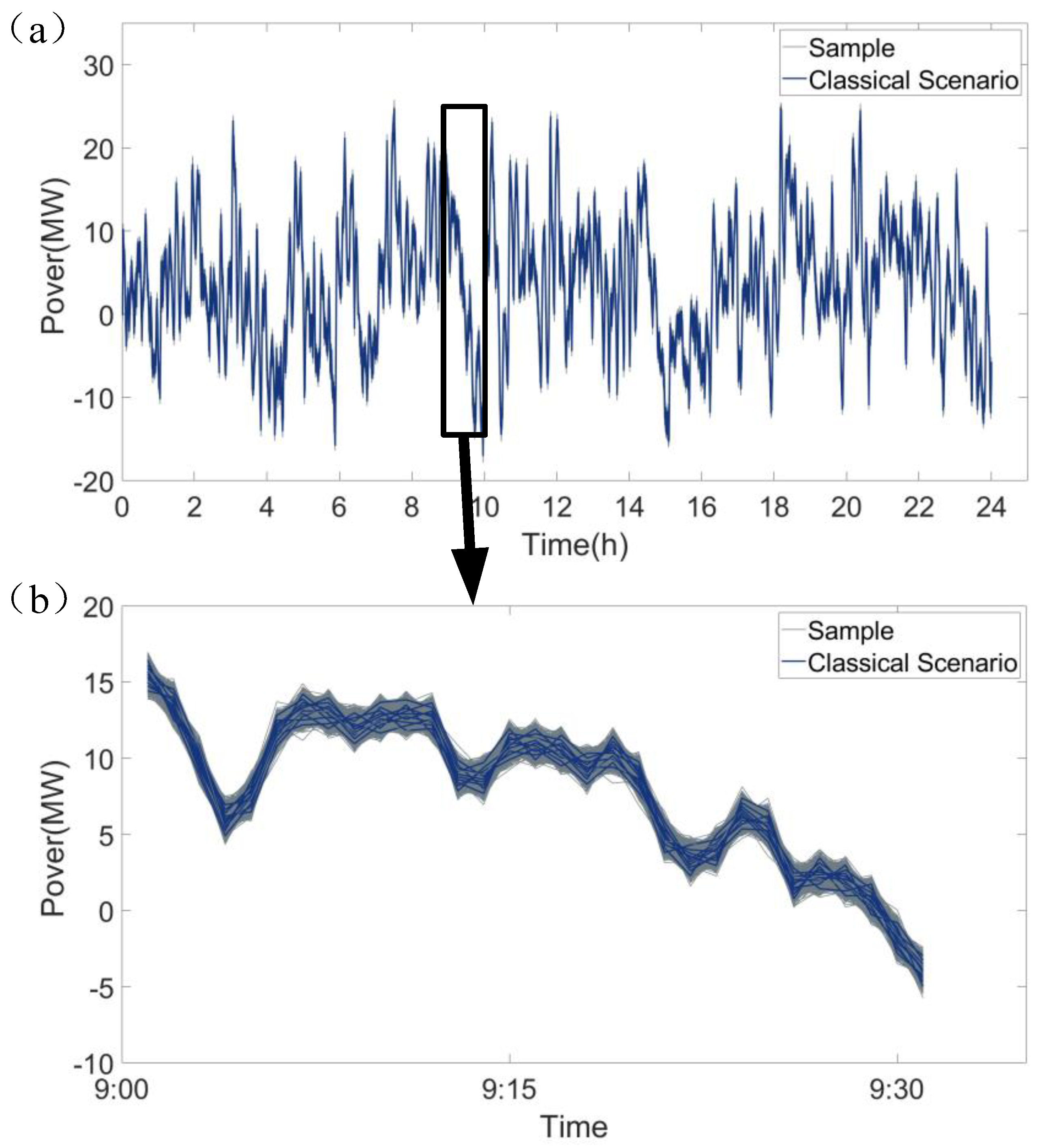
3.3. Scenario Generation and Reduction

The prediction accuracy can be improved by LSTM, but due to the influence of multiple factors of heavy railway traction power, it leads to there always being an error in the actual prediction value and the actual value. The possible scenario during actual operation is generated by LHS, and then a representative classical scenario is obtained by FCM.

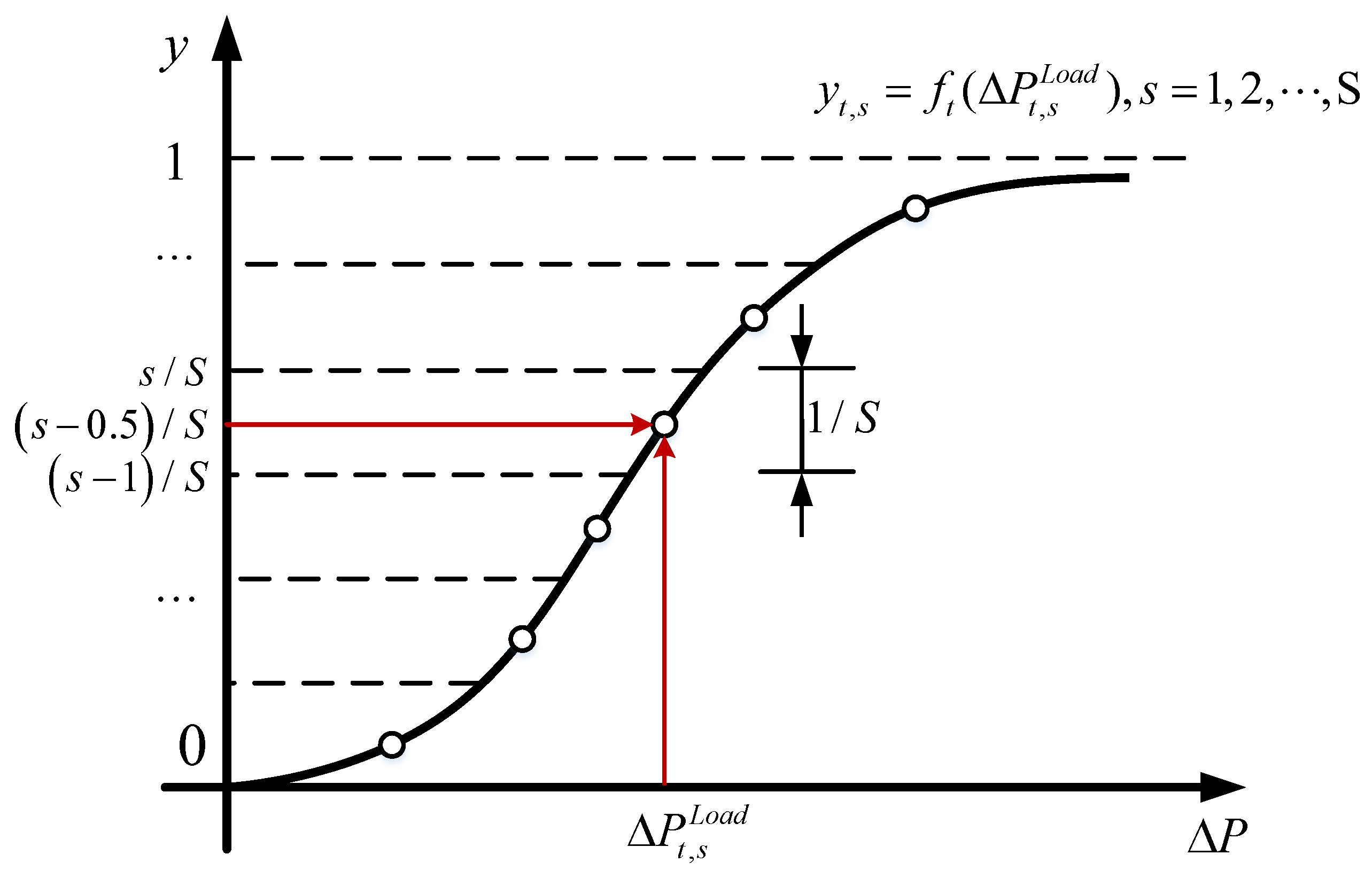
3.3.1. Latin Hypercube Sampling

LHS is a stratified approach to ensure that the entire distribution of each quantity is effectively covered [36,37]. This avoids the problem of excessive clustering of samples in a particular region that can occur in random sampling, thus reducing the error variance. The $\mathrm{\Delta }{P}_{t,s}^{Load}(t=1,···,T)$ is random input variables, Figure 4 is the probability cumulative function of $\mathrm{\Delta }{P}_{t,s}^{Load}$ and the probability cumulative function of the random variable $\mathrm{\Delta }{P}_{t,s}^{Load}$ is:

$$y_{t,s}=f_t\left(\mathrm{\Delta }{P}_{t,s}^{Load}\right),s=1,2,···,S$$

(10)

where S is the sample size. $f_t$ is the probability cumulative function of the random variable.

The longitudinal axis of the probability cumulative function curve is divided into K equally spaced regions, each of which has a length of $1/S$, and the value point in the region is chosen as $y_s$, which is brought into the inverse function of probability cumulative function to obtain the value of the random variable, which can be expressed as:

$$\mathrm{\Delta }{P}_{t,s}^{Load}=f_t^{-1}\left({\displaystyle \frac{s-0.5}{S}}\right)$$

(11)

where $f_t^{-1}$ is the inverse function of probability cumulative function.

After completing the sampling of all random variables, each random variable sampled value is arranged in a row to obtain all random variable sampling matrix $T\times S$, which can be expressed as:

$$\mathrm{\Delta }{P}_{T\times S}^{Load}=\left[\begin{array}{ccc}\mathrm{\Delta }{P}_{1,1}^{Load}& ···& \mathrm{\Delta }{P}_{1,S}^{Load}\\ ···& & ···\\ \mathrm{\Delta }{P}_{T,1}^{Load}& ···& \mathrm{\Delta }{P}_{T,S}^{Load}\end{array}\right]$$

(12)

3.3.2. Fuzzy C-Means

The fuzzy C-mean (FCM) clustering algorithm is a fuzzy clustering algorithm based on the objective function. The idea of the method uses the degree of affiliation to represent the relationship between each data. In traditional clustering algorithms, the affiliation degree to determine whether a variable belongs to a certain set of features is only 0 or 1. In fuzzy sets, the affiliation degree is not only 0 or 1, but also other numbers between 0–1, and a variable can belong to several different clusters [38].

For a given data sets: $\mathrm{\Delta }{P}_s^{Load}=\left\{\mathrm{\Delta }{P}_1^{Load},···,\mathrm{\Delta }{P}_s^{Load},···,\mathrm{\Delta }{P}_S^{Load}\right\}$, The FCM divides this dataset into N classes, N being a positive integer greater than 1, where the clustering center of N clusters is $\left[v_1,···,v_N\right]$. The objective function and constraints of the FCM are:

$$Obj=\sum _{i=1}^N\sum _{j=1}^S{\mu }_{ij}^m{∥\mathrm{\Delta }{P}_j^{Load}-v_i∥}^2$$

(13)

$$\sum _{i=1}^N{\mu }_{ij}=1,j=1,2,···,S$$

(14)

where $Obj$ is the objective function. $v_i,{\mu }_{ij}$ is the variables. n is the total number of samples, N is the number of cluster centers. $m(m>1)$ is the affiliation factor.

In order to minimize the objective function $Obj$, the Lagrange multiplier method is used on the objective function while satisfying the constraints to obtain the affiliation matrix ${\mu }_{ij}$ and the clustering center $v_i$, can be expressed as:

$${\mu }_{ij}={\displaystyle \frac{1}{{\displaystyle \sum _{b=1}^N}{\left(\frac{∥\mathrm{\Delta }{P}_j^{Load}-v_i∥}{∥\mathrm{\Delta }{P}_j^{Load}-v_b∥}\right)}^{\frac{2}{m-1}}}}$$

(15)

$$v_i={\displaystyle \frac{{\displaystyle \sum _{j=1}^S}\left({\mu }_{ij}^m\mathrm{\Delta }{P}_j^{Load}\right)}{{\displaystyle \sum _{j=1}^S}{\mu }_{ij}^m}}$$

(16)

The algorithm is described in detail below:

Step 1: Initialize the affiliation factor m, iteration error $\epsilon$, maximum number of iterations T and affiliation matrix ${\mu }_{ij}$. Randomly select N samples from the initial sample as initial clustering centers;

Step 2: Calculate or update the affiliation matrix U based on the Equation (15) and update the clustering center based on the Equation (16);

Step 3: Compare $Obj\left(t\right)$ and $Obj(t-1)$. If $∥Obj\left(t\right)-Obj(t-1)∥\le \epsilon$, then out put clustering center v and affiliation matrix U. Otherwise, $t=t+1$, return to Step 2 and continue iterating.

4. Stochastic Optimization Model for HFTPSS

Battery degradation and power uncertainty seriously affect the economic operation of HFTPSS. To consider the impact of battery degradation and power uncertainty on HFTPSS energy management. In this section, a stochastic optimization model of HFTPSS considering the online degradation of battery is established.

4.1. Objective Function

The stochastic optimization objective function Equation (17) is to minimize the expected average daily operation cost of the HFTPSS in the classical scenario. The first term, $C^{ECC}$ represents the expected cost of electricity in N classical scenario. Equation (19) represents the calculation of the maximum demand. $C^{DC}$ is the expected cost of demand. The third term in the objective function is the penalty cost for RBE feedback to the grid. $C^{BC}$ is the cost of degradation of battery. Since the charging and discharging strategy of ESS is the same in all scenarios, the degradation cost of ESS is the same in all scenarios.

$$C^{Total}=C^{ECC}+C^{DC}+C^{PC}+C^{BC}$$

(17)

$$C^{ECC}=\sum _{n=1}^N{\rho }_n\left(\sum _{t=1}^T{\lambda }_t^E·(P_{t,n}^{grid,A}+P_{t,n}^{grid,B})\right)$$

(18)

$$P_{t,n}^{dem,tra}=\sum _{t=1}^{t+14}{P}_{t,n}^{grid,tra}/15,tra\in \{A,B\}$$

(19)

$$C^{DC}={\lambda }^D·\sum _{n=1}^N{\rho }_{n}max\left(P_{t,n}^{dem,A}\right)+{\lambda }^D·\sum _{i=1}^N{\rho }_{n}max\left(P_{t,n}^{dem,B}\right)$$

(20)

$$C^{PC}=\sum _{n=1}^N{\rho }_n\left(\sum _{t=1}^T{\lambda }_t^P·(P_{t,n}^{feed,A}+P_{t,n}^{feed,B})\right)$$

(21)

$$C^{BC}={\lambda }^B\sum _{t=1}^T\left({\Gamma }_t^{cyc,A}+{\Gamma }_t^{cal,A}+{\Gamma }_t^{cyc,B}+{\Gamma }_t^{cal,B}+{\Gamma }_t^{cyc,NZ}+{\Gamma }_t^{cal,NZ}\right)$$

(22)

where ${\rho }_n$ is the probability that scenario n occurs. ${\lambda }_t^E,{\lambda }_t^P$, ${\lambda }^D$ is the purchased electricity price, penalty price, and the demand price. ${\lambda }^B$ is the degradation price of ESS. $P_{t,n}^{grid,A},P_{t,n}^{dem,A},P_{t,n}^{feed,A}$ is the active power supplied by the grid, demand power and RBE power of TSS-A, $P_{t,n}^{grid,B},P_{t,n}^{dem,B},P_{t,n}^{feed,B}$ is the active power supplied by the grid, demand power and RBE power of TSS-B. ${\mathrm{\Gamma }}_t^{cyc,A},{\mathrm{\Gamma }}_t^{cyc,B},{\mathrm{\Gamma }}_t^{cyc,NZ}$ is the cycle aging of the battery in TSS-A, TSS-B and NZ, respectively. ${\mathrm{\Gamma }}_t^{cal,A},{\mathrm{\Gamma }}_t^{cal,B},{\mathrm{\Gamma }}_t^{cal,NZ}$ is the calender aging of the battery in TSS-A, TSS-B and NZ, respectively.

4.2. Constraints

4.2.1. Power Flow Constraints

Power balance constraints of each port of HFTPSS in all scenario can be described in Equations (23)–(25). They represent the relationship between active power supplied by the grid for each TSS ($P_{t,n}^{grid}$), superfluous RBE fed back to the grid for each TSS ($P_{t,n}^{feed}$), charge or discharge power for each ESS ($P_{ch,t}^{bat},P_{dis,t}^{bat}$), output power of PFC ($P_t^{PFC,\alpha },P_t^{PFC,\beta }$).

$$P_{t,n}^{grid,A}+P_t^{PFC,\alpha }+P_{dis,t}^{bat,A}=P_{ch,t}^{bat,A}+P_{t,n}^{Load,A}+P_{t,n}^{feed,A}$$

(23)

$$P_{t,n}^{grid,B}+P_t^{PFC,\beta }+P_{dis,t}^{bat,B}=P_{ch,t}^{bat,B}+P_{t,n}^{Load,B}+P_{t,n}^{feed,B}$$

(24)

$$P_t^{PFC,\beta }+P_t^{PFC,\alpha }+P_{ch,t}^{bat,NZ}=P_{dis,t}^{bat,NZ}$$

(25)

4.2.2. Energy Storage Constraints

The characteristics of large-capacity ESS can realize the efficient use of RBE. The state and power limits of ESS can be set up from Equation (26a–f), which means that the ESS can only be in a charging or discharging state at one time, and its power cannot exceed the rated power. But the battery capacity cannot exceed the upper and lower limits of its rated capacity. The remaining capacity constraint, defined by the rate capacity of the battery, is shown in Equation (27a–c). Equation (28a–c) limit how the actual battery capacity $E_{t+1}^{bat}$ can mutate, it is influenced by the adjacent battery capacity $E_t^{bat}$ and charging or discharging power $P_{ch,t}^{bat},P_{dis,t}^{bat}$. At the same time, the battery maximum capacity is related to calendar aging and cycle aging, it can be expressed as Equation (29a–c).

$$0\le P_{ch,t}^{bat,A}\le {\mu }_t^{bat,A}·\overline{P^{bat,A}}$$

(26a)

$$0\le P_{dis,t}^{bat,A}\le \left(1-{\mu }_t^{bat,A}\right)·\overline{P^{bat,A}}$$

(26b)

$$0\le P_{ch,t}^{bat,B}\le {\mu }_t^{bat,B}·\overline{P^{bat,B}}$$

(26c)

$$0\le P_{dis,t}^{bat,B}\le \left(1-{\mu }_t^{bat,B}\right)·\overline{P^{bat,B}}$$

(26d)

$$0\le P_{ch,t}^{bat,NZ}\le {\mu }_t^{bat,NZ}·\overline{P^{bat,NZ}}$$

(26e)

$$0\le P_{dis,t}^{bat,NZ}\le \left(1-{\mu }_t^{bat,NZ}\right)·\overline{P^{bat,NZ}}$$

(26f)

$$Ca{p}^A·{SOC}^{min}\le E_t^{bat,A}\le Ca{p}^A·SO{C}^{max}$$

(27a)

$$Ca{p}^B·SO{C}^{min}\le E_t^{bat,B}\le Ca{p}^B·SO{C}^{max}$$

(27b)

$$Ca{p}^{NZ}·SO{C}^{min}\le E_t^{bat,NZ}\le Ca{p}^{NZ}·SO{C}^{max}$$

(27c)

$$E_{t+1}^{bat,A}=\left(1-\delta \right)·E_t^{bat,A}+{\epsilon }_{ch}·P_{ch,t}^{bat,A}·\mathrm{\Delta }t-{\displaystyle \frac{P_{dis,t}^{bat,A}}{{\epsilon }_{dis}}}·\mathrm{\Delta }t$$

(28a)

$$E_{t+1}^{bat,A}=\left(1-\delta \right)·E_t^{bat,A}+{\epsilon }_{ch}·P_{ch,t}^{bat,A}·\mathrm{\Delta }t-{\displaystyle \frac{P_{dis,t}^{bat,A}}{{\epsilon }_{dis}}}·\mathrm{\Delta }t$$

(28b)

$$E_{t+1}^{bat,A}=\left(1-\delta \right)·E_t^{bat,A}+{\epsilon }_{ch}·P_{ch,t}^{bat,A}·\mathrm{\Delta }t-{\displaystyle \frac{P_{dis,t}^{bat,A}}{{\epsilon }_{dis}}}·\mathrm{\Delta }t$$

(28c)

$$E_{act,t+1}^{bat,A}=E_{act,t}^{bat,A}-{\mathrm{\Gamma }}_t^{cyc,A}-{\mathrm{\Gamma }}_t^{cal,A}$$

(29a)

$$E_{act,t+1}^{bat,B}=E_{act,t}^{bat,B}-{\mathrm{\Gamma }}_t^{cyc,B}-{\mathrm{\Gamma }}_t^{cal,B}$$

(29b)

$$E_{act,t+1}^{bat,NZ}=E_{act,t}^{bat,NZ}-{\mathrm{\Gamma }}_t^{cyc,NZ}-{\mathrm{\Gamma }}_t^{cal,NZ}$$

(29c)

where $\overline{P^{bat,A}},\overline{P^{bat,b}},\overline{P^{bat,NZ}}$ is the maximum power for each battery. ${\mu }_t^{bat,A},{\mu }_t^{bat,B},{\mu }_t^{bat,NZ}$ is the binary variable, which determines whether the battery is in a charging or discharging state. $Ca{p}^A,Ca{p}^B,Ca{p}^{NZ}$ is the rate capacity of each battery. $SO{C}^{min},SO{C}^{max}$ is the minimum and maximum SOC of battery. $E_t^{bat,A},E_t^{bat,B},E_t^{bat,NZ}$ is the capacity of each battery at time t.${\epsilon }_{ch},{\epsilon }_{dis}$ is the battery charging and discharging efficiency. $E_{act,t}^{bat,A},E_{act,t}^{bat,B},E_{act,t}^{bat,ZN}$ are the maximum capacities of the battery in TSS-A, TSS-B and NZ at time t, respectively.

4.3. Online Degradation of Battery

The ESS consisting of a battery has the characteristic of high capacity density and can absorb a large amount of RBE. However, overuse of the battery will accelerate battery aging. It is recommended to replace the battery when its capacity deteriorates to 80% of its rate capacity [39]. Considering the economic optimization of HFTPSS operation under battery degradation, a mathematical model of the effect of charging and discharging power on battery degradation is established.

4.3.1. Calendar Aging of Battery

Calendar aging of the battery is affected by several factors, such as temperature, battery SOC, battery action duration, and other factors. In this paper, the impact of battery calendar aging on optimal scheduling is considered. According [39], the linearized function of the battery calendar aging is:

$${\mathrm{\Gamma }}_t^{cal}=\left[{\left({\displaystyle \frac{t-1}{720}}\right)}^{0.8}-{\left({\displaystyle \frac{t-1}{720}}\right)}^{0.8}\right]\left({\kappa }_1·{SOC}_t+{\kappa }_2·E_{act,t}^{bat}\right)$$

(30)

where ${\mathrm{\Gamma }}_t^{cal}$ is the calendar aging at time t. ${\kappa }_1,{\kappa }_2$ is the degradation factor. ${SOC}_t$ is the SOC of battery at time t. $E_{act,t}^{bat}$ is the actual capacity of battery at time t.

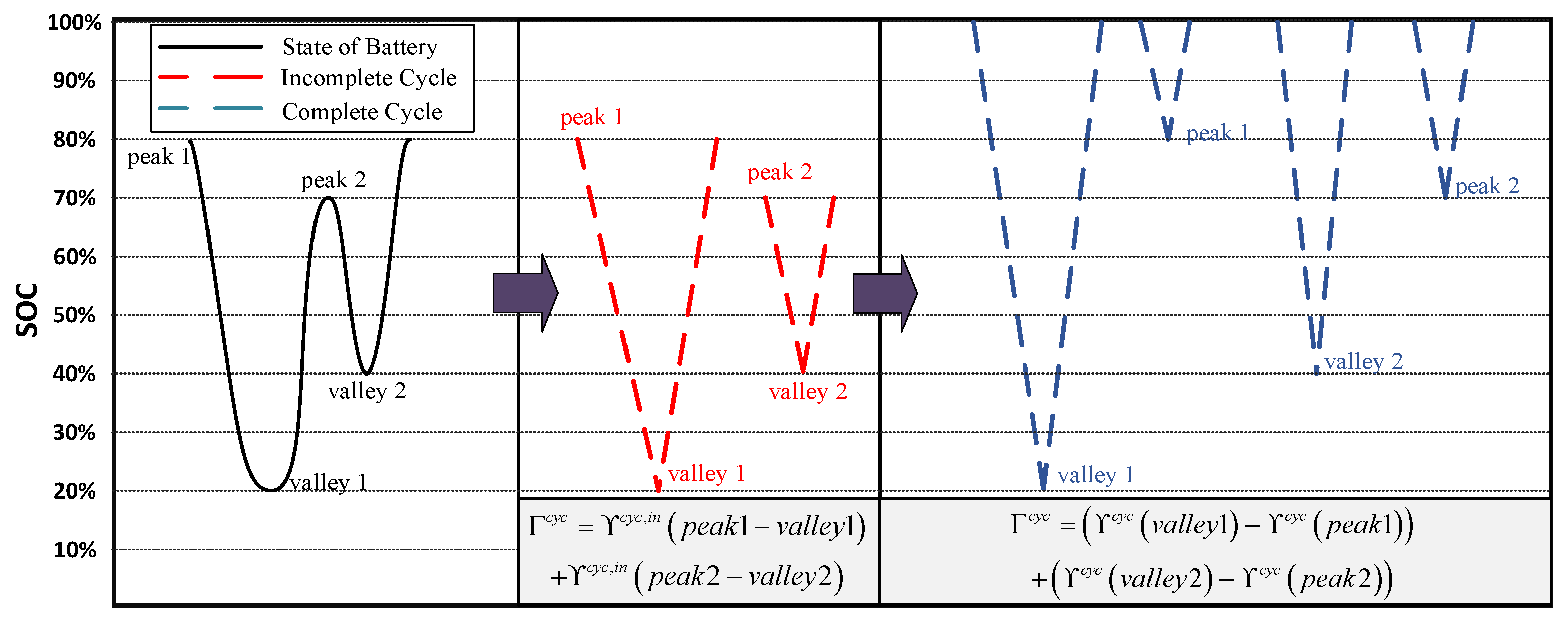
4.3.2. Cycle Aging of Battery

Frequent charging and discharging of the battery and the DOD per cycle will seriously affect the cycle life of the battery. This section only considers the effect of DOD on cycle life, ignoring other environmentally induced battery degradation. In [40], the relationship between the number of battery cycles and DOD can be expressed as:

$$N^{cyc}={\chi }_1·DO{D}^{-{\chi }_2}·e^{{\chi }_3(1-DOD)}$$

(31)

where ${\chi }_1,{\chi }_2,{\chi }_3$ is the fitting curve coefficients. They can be obtained through the battery manufacturer.

We consider the effect of each charging and discharging row of the battery on the degradation of the battery independently. At the same time, consider replacing the battery when its capacity deteriorates to 80% of the initial capacity. Therefore, the capacity degradation affected by charging and discharging can be expressed as:

$${\mathrm{Y}}^{cyc}={\displaystyle \frac{0.2·Cap}{N^{cyc}}}$$

(32)

Battery cycling can be categorized into complete cycles and incomplete cycles. The number of complete cycles and incomplete cycles of the battery is obtained by the rainflow cycle counting algorithm. The complete cycle aging can be calculated by Equation (32). In order to solve the incomplete cycle aging problem, Ref. [39] utilizes the superposition theorem to estimate the cyclic aging of an incomplete cycle by converting one incomplete cycle into two complete cycles. As shown in Figure 5, the incomplete cycle can be obtained by the subtraction of two complete cycles. Then, the battery cycle aging can be expressed as:

$${\mathrm{\Gamma }}_t^{cyc}=({\mathrm{Y}}_t^{cyc}-{\mathrm{Y}}_{peak}^{cyc})·{\mu }_t$$

(33)

where ${\mu }_t$ is the binary variable indicating the state of the battery from discharging to charging. ${\mathrm{Y}}_{peak}^{cyc}$ is the nearest SOC peak before time t.

We consider $\mathrm{Y}$ as a function with respect to $SOC$, $SOC=1-DOD$. It can be expressed as:

$$SO{C}_t={\displaystyle \frac{E_t^{Bat}}{Cap}}$$

(34)

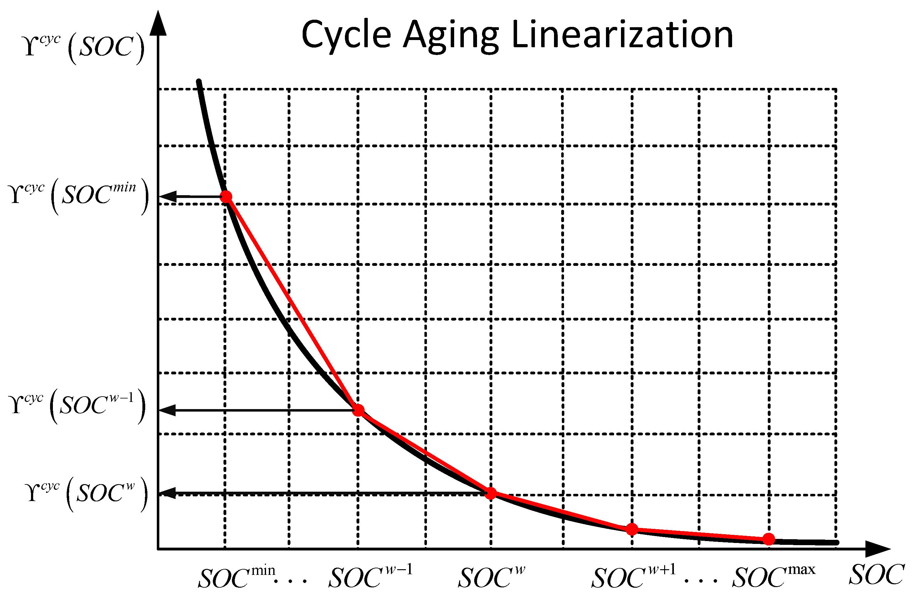
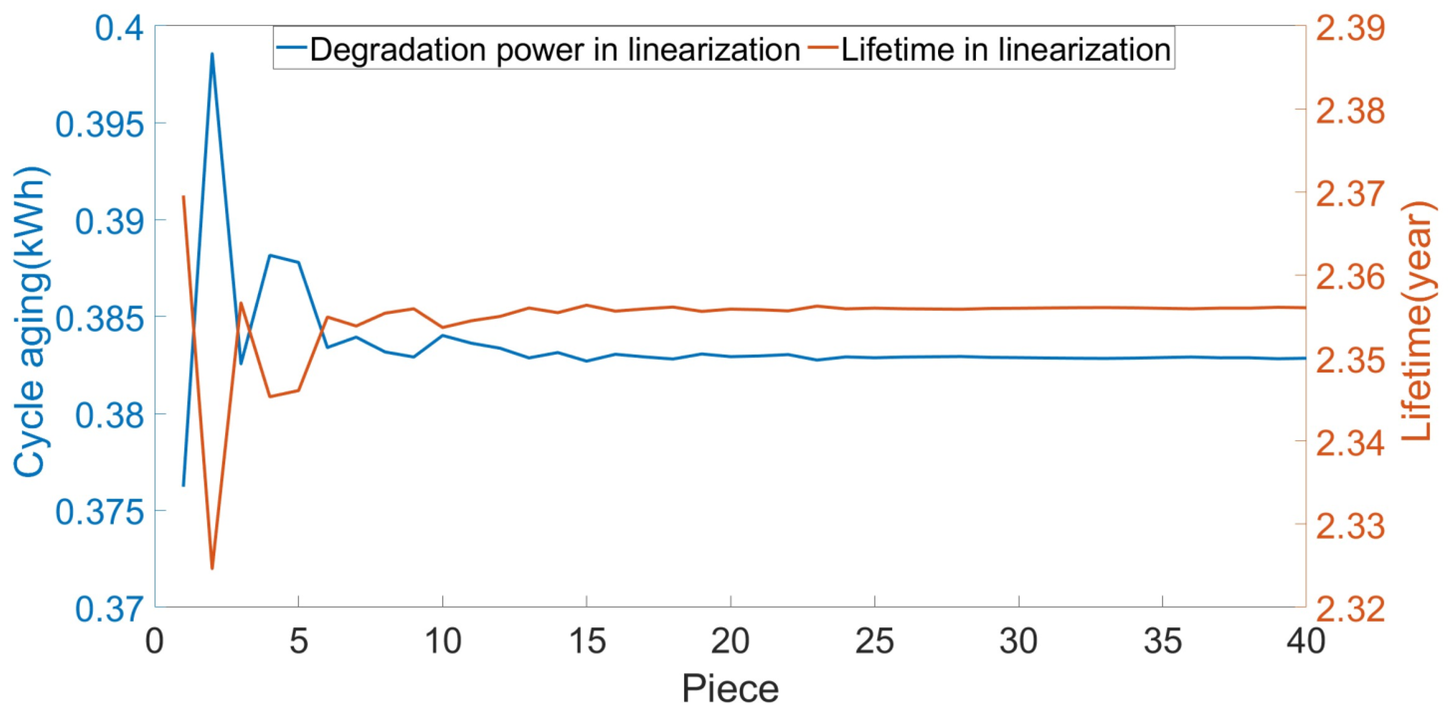
4.4. Linearization of Battery Degradation

Since the battery degradation process is a nonlinear process, as shown in Figure 6, a segmented linearization approach is used to model the battery degradation as a segmented function:

$${\mathrm{Y}}^{cyc}\left(SO{C}_t\right)=\left\{\begin{array}{c}{\mathrm{Y}}^{cyc,1}\left(SO{C}_t\right),SO{C}_t\in \left[SO{C}^{min},SO{C}^{min}+L\right]\hfill \\ ···\hfill \\ {\mathrm{Y}}^{cyc,w}\left(SO{C}_t\right),SO{C}_t\in \left[SO{C}^{min}+(w-1)·L,SO{C}^{min}+w·L\right]\hfill \\ ···\hfill \\ {\mathrm{Y}}^{cyc,W}\left(SO{C}_t\right),SO{C}_t\in \left[SO{C}^{max}-L,SO{C}^{max}\right]\hfill \end{array}\right.$$

(35)

$$\begin{array}{c}{\mathrm{Y}}^{cyc,w}\left(SO{C}_t\right)={\displaystyle \frac{{\mathrm{Y}}^{cyc}\left(SO{C}^{min}+(w-1)·L\right)-{\mathrm{Y}}^{cyc}\left(SO{C}^{min}+w·L\right)}{L}}\hfill \\ ·\left(SO{C}_t-SO{C}^{min}-w·L\right)+{\mathrm{Y}}^{cyc}\left(SO{C}^{min}+(w-1)·L\right)\hfill \end{array}$$

(36)

where W is the number of segmented functions. L is the length of each segment function, $L=(SO{C}^{max}-SO{C}^{min})/W$.

Further, ${\upsilon }_t^w$ binary variables are introduced to represent the segmented function:

$$\sum _{w=1}^W{\upsilon }_t^w=1$$

(37)

$$0\le Y_t^{cyc,w}\le M·\left(1-{\upsilon }_t^w\right),w\in [1,W]$$

(38)

$${\mathrm{Y}}_t^{cyc,w}-M·{\upsilon }_t^w\le Y_t^{cyc,w}\le {\mathrm{Y}}_t^{cyc,w}+M·{\upsilon }_t^w$$

(39)

where Equation (37) denotes the line segment which $SOC$ belong to at time t.

Then, linearization of Equation (32) leads to the following equation:

$${\mathrm{Y}}_t^{cyc}=\sum _{w=1}^W{Y}_t^{cyc,w}$$

(40)

Further, Equation (33) can be accurately expressed by the big M method as:

$$0\le {\mathrm{\Gamma }}_t^{cyc}\le M·\left(1-{\mu }_t\right)$$

(41)

$$\left({\mathrm{Y}}_t^{cyc}-{\mathrm{Y}}_{peak}^{cyc}\right)-M·{\mu }_t\le {\mathrm{\Gamma }}_t^{cyc}\le \left({\mathrm{Y}}_t^{cyc}-{\mathrm{Y}}_{peak}^{cyc}\right)+M·{\mu }_t$$

(42)

5. Case Study

5.1. System Parameter Setting

In this section, the MILP model of this paper is represented. The solution was performed in the MATLAB 2023b software environment using the integrated YALMIP toolbox and the Gurobi solver 10.0.3 interface on a workstation with 12th Gen Intel(R) Core(TM) i7-12700H CPU and 16 GB RAM. The validity of the method is verified by analyzing the optimization rate of the total system electricity cost and battery life.

The actual operation data of two tractions in HERs is considered for a case study. The tariff parameters table and battery parameters are shown in

Table 1. Tariff Parameters.

Time Pired	0:00–6:00 22:00–0:00	8:00–11:00 18:00–21:00	Others
Energy ($/kWh)	0.051	0.172	0.108
Demand ($/kWh/mon)	5.785	5.785	5.785

and

Table 2. Battery Parameters.

Parameters	Initial SOC	Efficiency	SOC Range	Self Discharge Rate (/mon )
Battery	0.5	0.85/0.85	0.2/0.8	0.05

. The optimal capacity configuration of the battery is: rated capacity 5 MWh and rated power 2 MW from Ref. [41]. According to Ref. [39], battery calendar aging factors are: ${\kappa }_1=0.0028,$ ${\kappa }_2=0.001939$. Battery cycle aging factors are: ${\chi }_1=3832,{\chi }_2=0.68,{\chi }_3=1.64$ from Ref. [42]. The capacity of the PFC is 20 MW. The degradation price of ESS ${\lambda }^B$ is cost of battery replacement, ${\lambda }^B$ = 904.4 $/kWh.

5.2. Performance of Uncertainty Modeling

In order to verify the prediction performance of the proposed model. The training and prediction testing work were performed from Recurrent Neural Network (RNN) and LSTM for historical data, respectively. The traction power for the past month was used as the dataset, with a time step of 1 min and a feature dimension of 1440. The number of hidden nodes in the network is 50. The prediction outcomes of each model are shown in Figure 7.

Table 3. Forecast Evaluation Index of Models.

MODEL	MAPE	RMSE	${\mathit{R}}^2$	PCC
LSTM	1.2592	1.6243	0.9551	0.9774
RNN	3.0225	3.7794	0.7563	0.9040

comparison error analysis of each model according Equation (43), including root mean square error (RMSE), mean absolute percentage error (MAPE), r-squared score ($R^2$), Pearson correlation coefficient (PCC). It can be seen that LSTM has better prediction accuracy.

$$\mathrm{RMSE}=\sqrt{{\displaystyle \frac{1}{n}}{\sum _{i=1}^n\left(y_i^{act}-y_i^{pre}\right)}^2}$$

(43a)

$$\mathrm{MAPE}={\displaystyle \frac{1}{n}}\sum _{i=1}^n\left|y_i^{act}-y_i^{pre}\right|$$

(43b)

$$R^2=1-{\displaystyle \frac{{{\displaystyle \sum _{i=1}^n}\left(y_i^{act}-y_i^{pre}\right)}^2}{{{\displaystyle \sum _{i=1}^n}\left(\overline{y_i^{act}}-y_i^{act}\right)}^2}}$$

(43c)

$$\mathrm{PCC}={\displaystyle \frac{{\displaystyle \sum _{i=1}^n}\left(y_i^{act}-\overline{y_i^{act}}\right)\left(y_i^{pre}-\overline{y_i^{pre}}\right)}{\sqrt{{{\displaystyle \sum _{i=1}^n}\left(y_i^{act}-\overline{y_i^{act}}\right)}^2}\sqrt{{{\displaystyle \sum _{i=1}^n}\left(y_i^{pre}-\overline{y_i^{pre}}\right)}^2}}}$$

(43d)

The prediction error will increase as the window slides. Thus, in this paper, the traction power prediction error is considered to be normally distributed, and the set of scenarios is sampled by the LHS method. The generated scenarios are shown in Figure 8.

With LHS, we can obtain huge sets of scenarios of traction power. However, the huge scenario will be a huge burden on the optimization solution. Therefore, we perform scene reduction by the FCM algorithm to obtain a classical scenario of power. The set of classical scenarios aggregated through FCM is shown in Figure 8.

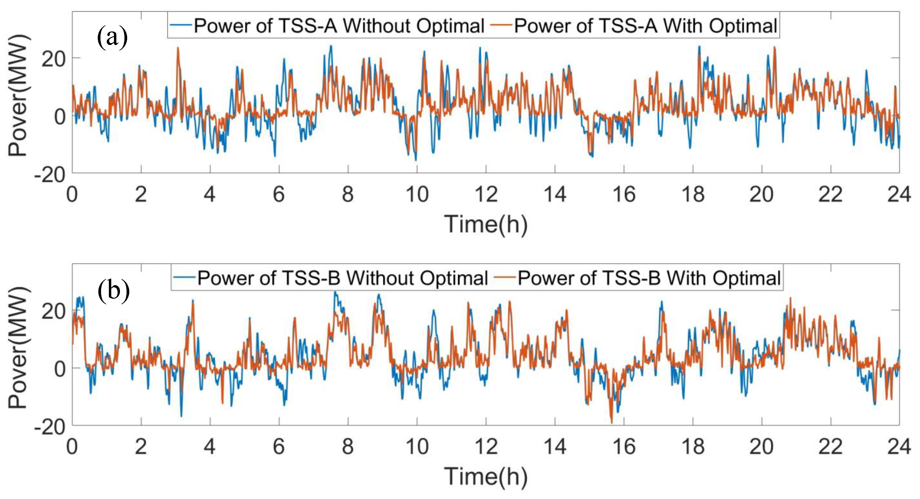
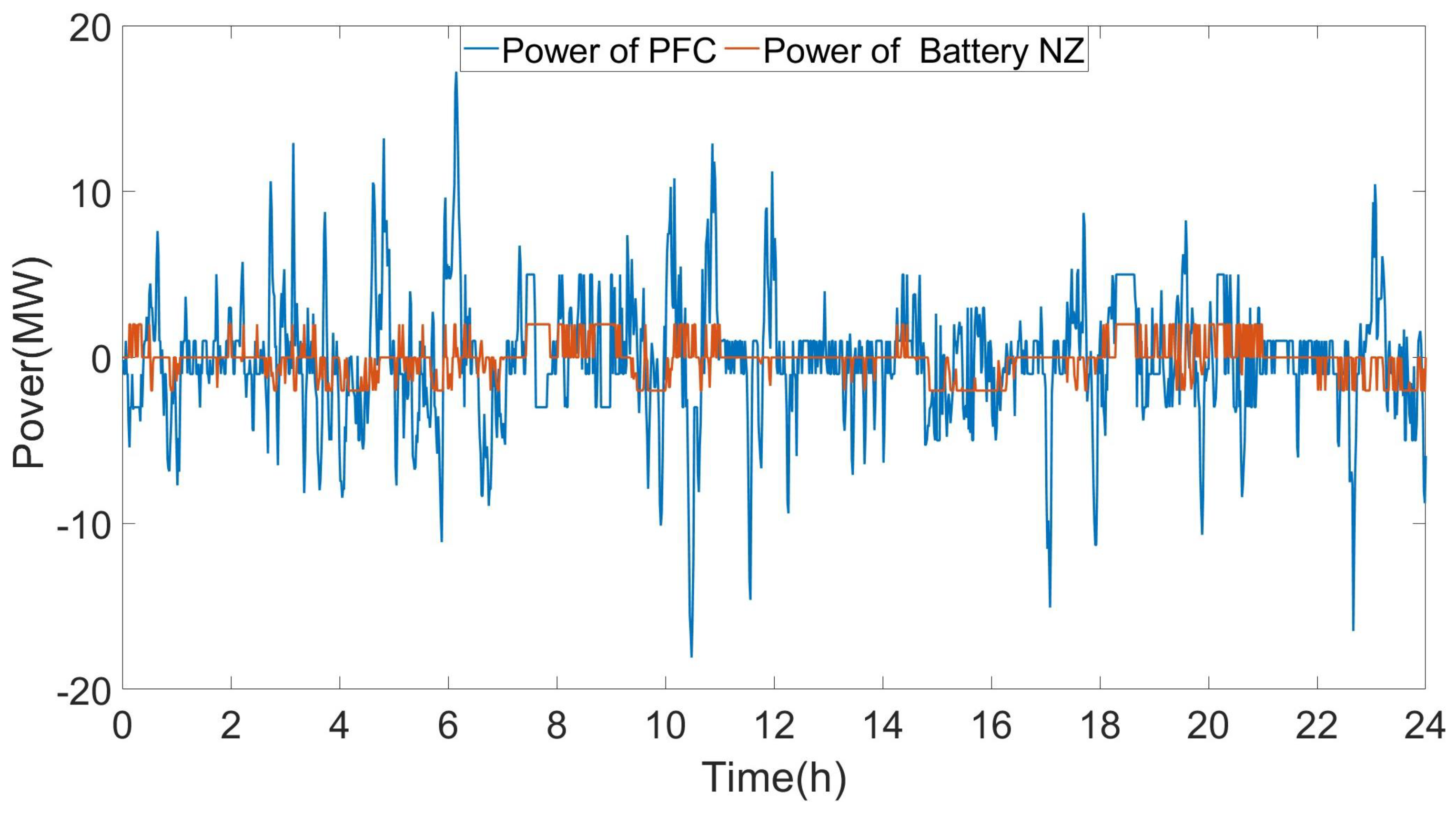
5.3. Performance of Stochastic Optimization Model

Based on the classical traction power scenario in the previous section. Analyze the costs obtained under the model proposed in this paper. Railroad electricity rates are based on the two-part electricity price and take into account the cost of penalties for the excess RBE return to the grid. Figure 9 compares the traction load with the power drawing from the grid side at the model proposed in this paper. Figure 9a shows the comparison of power before and after optimization of TSS−A; it can be seen that by controlling the charging and discharging state of the ESS and the input or output power of the PFC, it can realize the peak shaving and valley filling of the TSS−A load.

Figure 10 shows the output power of PFC and battery. PFC realizes the power flow between the stations. It can be seen that the utilization of excess RBE is achieved by the PFC. Reducing the cost of penalties caused by returning excess RBE to the grid. At the same time, access to the ESS at the PFC enables the flexible flow of energy.

Figure 11 demonstrates the relationship between capacity degradation and charging and discharging states of battery A. Affected by peak and valley tariffs, the battery discharges during peak price periods until its remaining capacity reaches the lower limit, thereby reducing power drawn from the grid and effectively lowering the system’s electricity costs. Moreover, charging is performed when the RBE is sufficient. According to Figure 11b. Under the influence of battery cycle aging, the capacity of the battery decreases faster when discharged. From 7:30 to 9:30, the battery’s capacity degradation due to the superposition of cyclic aging and calendar aging is 0.17589 kWh. At the same time, the capacity of the battery decreases slower when the battery is charging or not having any action. The degradation capacity of the battery under calendar aging from 15:30 to 17:30 is only 0.06844 kWh.

Finally, it can be seen that after a full day of scheduling, the available capacity of battery A is 4998.839 kWh, which means the degradation of capacity is 1.161 kWh. The daily operating costs of HFTPSS are shown in the

Table 4. Comparison of Operating Cost.

Cost ($)	ECC		DC		PC		BC			Total Cost
	TSS-A	TSS-B	TSS-A	TSS-B	TSS-A	TSS-B	Bat-A	Bat-B	Bat-NZ
Without Optimal	12,750	15,136	3030	4195	2068	2064	-	-	-	39,243
With Optimal	11,461	13,588	2299	3163	820	935	1026	1036	1023	35,351

. Of this, the cost of electricity (ECC) was reduced by 10.17%. The cost of demand (DC) was reduced by 24.4% and the penalty cost (PC) was reduced by 57.5%. Approximately 9.9% reduction in total cost.

5.4. Sensitivity Analysis

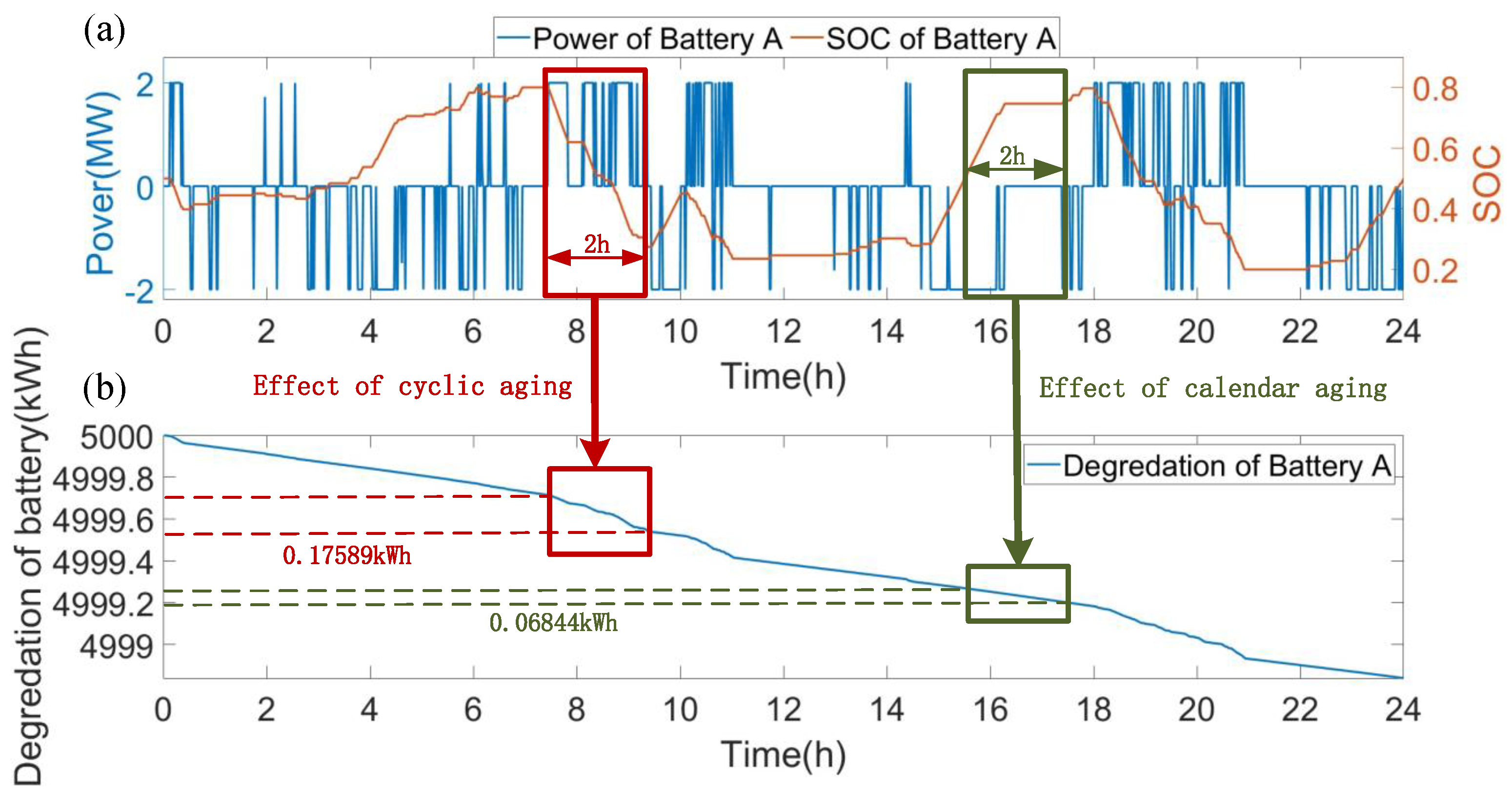
5.4.1. Battery Degradation Analysis

In this paper, a segmented linearization approach is used to deal with nonlinear problems in cyclic aging. By comparing with optimization without considering battery degradation Ref. [41]. It can be seen that the battery capacity degradation is more pronounced under a scheduling strategy that does not consider the effects of battery degradation. The system costs are shown in the

Table 5. Battery Degradation Result.

Model	Capacity Degradation (kWh)						Cost of Degradation ($)		Total Cost ($)
	Canlder Aging			Cycle Aging			Canlder Aging	Cycle Aging
	A	B	NZ	A	B	NZ
Model in this paper	0.778	0.773	0.778	0.383	0.399	0.376	2062	1023	35,351
Model in [41]	0.774	0.775	0.776	0.448	0.448	0.45	2058	1191	35,416

. After considering the online degradation of the battery in this paper, the degradation capacity of battery A is reduced from 0.448 kWh to 0.383 kWh, the degradation capacity of battery B is reduced from 0.448 kWh to 0.399 kWh, and the degradation capacity of battery NZ is reduced from 0.45 kWh to 0.376 kWh. The total system battery degradation cost is reduced from 3249$ to 3085$. Reduced cycle aging costs by 13.9%. The proportion of battery degradation cost decreased from 9.17% to 8.73%. Total system operating cost savings of 65$.

The nonlinear model of battery capacity degradation is transformed into a linear model is established by the method of segmental linearization and solved by MILP. The figure demonstrates the cycle aging size of battery A under different numbers of segments. It can be seen that the cycle aging and lifetime converge with the add of pieces in Figure 12. At a segmentation number of 15, the battery cycle aging and life are essentially unchanged. Therefore, take 20 for the number of pieces in this paper.

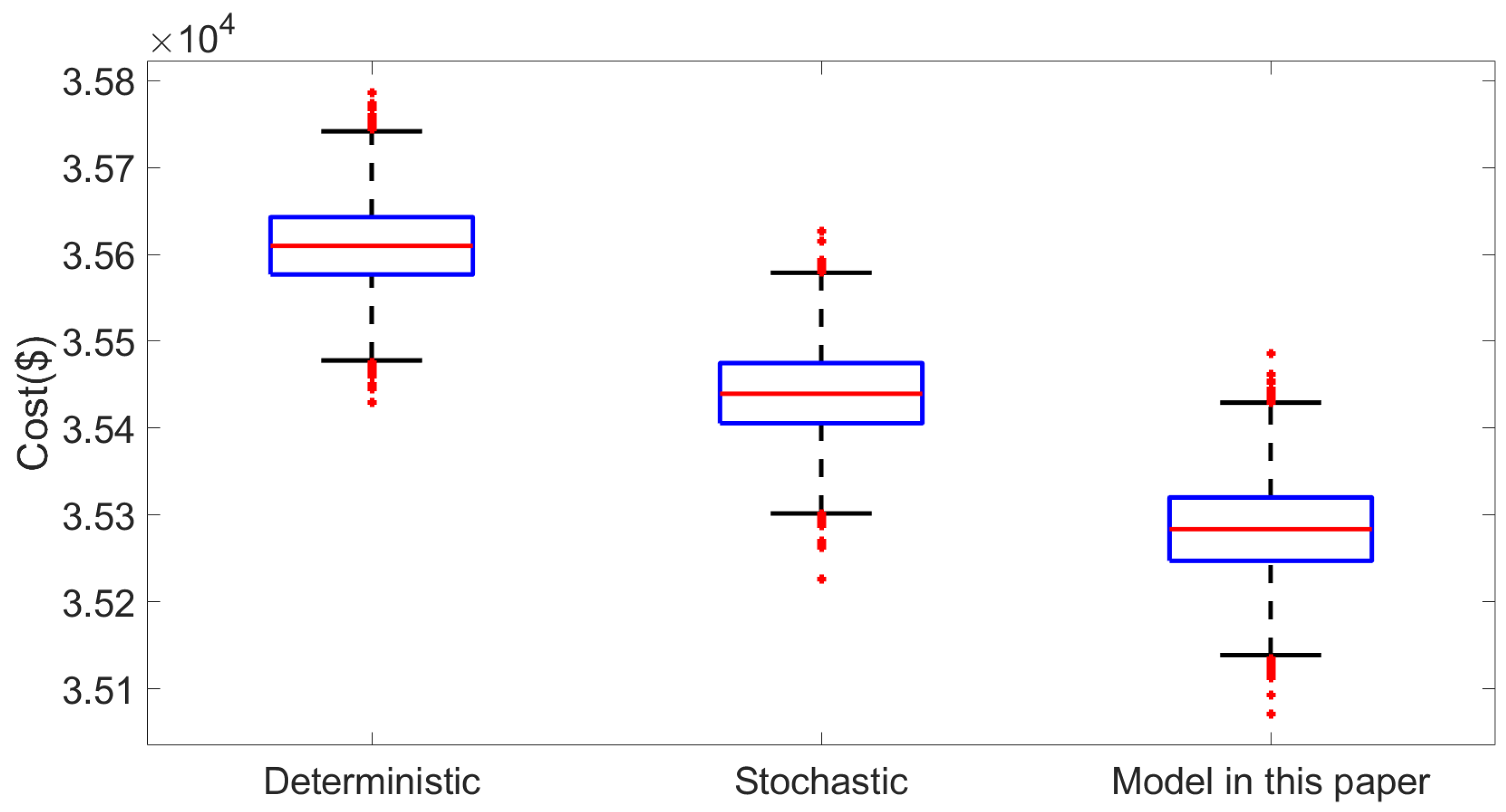
5.4.2. Economy and Robustness Analysis

In order to verify the economy and robustness of the stochastic programming model proposed in this paper. First, actual operational scenarios are simulated by sampling as the set of test scenarios in Figure 13. Then, the model proposed in this paper is solved to obtain the optimal scheduling strategy of the system. The scheduling strategy is brought into the test scenarios to calculate the operating costs under each scenario. The number of the set of test scenarios is 50,000. And, comparing the model of this paper with the deterministic optimization model proposed in Ref. [43] and a classical scene generation model based on Monte Carlo and k-means algorithm proposed in Ref. [44].

Figure 14 reflects the effects of deterministic optimization and stochastic optimization. And compare the cost distribution of the set of test scenarios under the model proposed in this paper with the deterministic optimization model in Ref. [43] and the stochastic optimization model based on Monte Carlo and k-means in Ref. [44]. It can be seen that the system has better robustness and economy under stochastic optimization. Compared with the deterministic optimization, the average costs have decreased by 0.8%. The lower cost under the stochastic optimization model in this paper indicates that the classical scenario generation method can obtain classical scenarios that reflect the characteristics of random variables.

6. Conclusions

This paper proposes a stochastic optimal scheduling strategy for HFTPSS that accounts for the online degradation of energy storage. The model incorporates the impact of battery degradation costs and the stochastic of traction power in scheduling the HFTPSS. To address the stochastic nature of traction power, a classical scenario generation method is proposed, integrating LSTM, LHS, and FCM to generate scenarios that reflect power characteristics. A stochastic optimal operation model is established for the HFTPSS to derive the charging and discharging strategy for the ESS and the control strategy for the PFC. Additionally, a battery aging model is developed, accounting for the effects of calendar and cyclic aging on battery capacity. The nonlinear battery degradation model is linearized using a segmental linearization method. Analysis of the case study indicates that the battery cycle aging cost is reduced by 13.9%. The effectiveness of the proposed classical scenario generation method is validated through comparative analysis. However, the above studies have not considered the impact of environmental factors on battery lifespan. In the future, system optimization and operation will be further explored under the influence of environmental conditions on battery longevity.

References

1. International Energy Agency. The Future of Rail; OECD: Paris, France, 2019; p. 175. [Google Scholar] [CrossRef]
2. Zhang, Z.; Sun, P.; Wei, M.; Wang, Q.; Feng, X. Trajectory Optimization for Heavy Haul Train with Pneumatic Braking via QCMIP. IEEE Trans. Intell. Veh. 2024, 9, 2419–2428. [Google Scholar]
3. Shunkai, L. Research and Application of Regenerative Braking Energy Utilization Scheme for Heavy Haul Railway. China Railw. 2022, 11, 45–54. [Google Scholar]
4. Zhao, S.; Li, K.; Yu, J.; Xing, C. Scheduling of futuristic railway microgrids—A FRA-pruned twins-actor DDPG approach. Energy 2024, 313, 134089. [Google Scholar] [CrossRef]
5. Milićević, S.; Blagojević, I.; Milojević, S.; Bukvić, M.; Stojanović, B. Numerical Analysis of Optimal Hybridization in Parallel Hybrid Electric Powertrains for Tracked Vehicles. Energies 2024, 17, 3531. [Google Scholar] [CrossRef]
6. Chen, Y.; Chen, M.; Xu, L.; Liang, Z. Chance-Constrained Optimization of Storage and PFC Capacity for Railway Electrical Smart Grids Considering Uncertain Traction Load. IEEE Trans. Smart Grid 2024, 15, 286–298. [Google Scholar] [CrossRef]
7. Han, Y.; Li, Q.; Wang, T.; Chen, W.; Ma, L. Multisource Coordination Energy Management Strategy Based on SOC Consensus for a PEMFC–Battery–Supercapacitor Hybrid Tramway. IEEE Trans. Veh. Technol. 2018, 67, 296–305. [Google Scholar] [CrossRef]
8. Chen, Y.; Chen, M.; Lu, W.; Egea-Àlvarez, A.; Xu, L. Improving energy efficiency for suburban railways: A two-stage scheduling optimization in a rail-EV smart hub. eTransportation 2024, 22, 100366. [Google Scholar] [CrossRef]
9. Pilo, E.; Mazumder, S.K.; González-Franco, I. Smart Electrical Infrastructure for AC-Fed Railways with Neutral Zones. IEEE Trans. Intell. Transp. Syst. 2015, 16, 642–652. [Google Scholar] [CrossRef]
10. Aguado, J.A.; Sánchez Racero, A.J.; de la Torre, S. Optimal Operation of Electric Railways with Renewable Energy and Electric Storage Systems. IEEE Trans. Smart Grid 2018, 9, 993–1001. [Google Scholar] [CrossRef]
11. Novak, H.; Lešić, V.; Vašak, M. Hierarchical Model Predictive Control for Coordinated Electric Railway Traction System Energy Management. IEEE Trans. Intell. Transp. Syst. 2019, 20, 2715–2727. [Google Scholar] [CrossRef]
12. Chen, M.; Cheng, Z.; Liu, Y.; Cheng, Y.; Tian, Z. Multitime-Scale Optimal Dispatch of Railway FTPSS Based on Model Predictive Control. IEEE Trans. Transp. Electrif. 2020, 6, 808–820. [Google Scholar] [CrossRef]
13. Chen, M.; Lv, Y.; Lu, W.; Zhang, D.; Chen, Y. Train-Network-HESS Integrated Optimization for Long-Distance AC Urban Rail Transit to Minimize the Comprehensive Cost. IEEE Trans. Intell. Transp. Syst. 2023, 24, 54–67. [Google Scholar] [CrossRef]
14. EN 50388; Railway Applications. Power Supply and Rolling Stock. Technical Criteria for the Coordination Between Power Supply (Substation) and Rolling Stock to Achieve Interoperability. BSI-Standards: London, UK, 2010; pp. 1–44.
15. Kummerow, A.; Klaiber, S.; Nicolai, S.; Bretschneider, P.; System, A. Recursive analysis and forecast of superimposed generation and load time series. In Proceedings of the International ETG Congress 2015; Die Energiewende-Blueprints for the New Energy Age, Bonn, Germany, 17–18 November 2015; pp. 1–6. [Google Scholar]
16. Christiaanse, W.R. Short-Term Load Forecasting Using General Exponential Smoothing. IEEE Trans. Power Appar. Syst. 1971, PAS-90, 900–911. [Google Scholar] [CrossRef]
17. Kalra, S.; Beniwal, R.; Singh, V.; Beniwal, N.S. Innovative Approaches in Residential Solar Electricity: Forecasting and Fault Detection Using Machine Learning. Electricity 2024, 5, 585–605. [Google Scholar] [CrossRef]
18. Liu, L.; Guo, K.; Chen, J.; Guo, L.; Ke, C.; Liang, J.; He, D. A Photovoltaic Power Prediction Approach Based on Data Decomposition and Stacked Deep Learning Model. Electronics 2023, 12, 2764. [Google Scholar] [CrossRef]
19. Song, K.B.; Baek, Y.S.; Hong, D.H.; Jang, G. Short-term load forecasting for the holidays using fuzzy linear regression method. IEEE Trans. Power Syst. 2005, 20, 96–101. [Google Scholar] [CrossRef]
20. Aneiros, G.; Vilar, J.; Raña, P. Short-term forecast of daily curves of electricity demand and price. Int. J. Electr. Power Energy Syst. 2016, 80, 96–108. [Google Scholar] [CrossRef]
21. Ma, Q.; Peng, Y.; Luo, P.; Li, Q.; Sun, J.; Wang, H. Electrified Railway Traction Load Prediction Based on Deep Learning. In Proceedings of the IECON 2020 The 46th Annual Conference of the IEEE Industrial Electronics Society, Singapore, 18–21 October 2020; pp. 4679–4684. [Google Scholar]
22. Yu, F.; Xu, X. A short-term load forecasting model of natural gas based on optimized genetic algorithm and improved BP neural network. Appl. Energy 2014, 134, 102–113. [Google Scholar] [CrossRef]
23. Wang, W.; He, Y.; Xiong, X.; Chen, H. Robust Survivability-Oriented Scheduling of Separable Mobile Energy Storage and Demand Response for Isolated Distribution Systems. IEEE Trans. Power Deliv. 2022, 37, 3521–3535. [Google Scholar] [CrossRef]
24. Li, J.; Du, Z.; Yuan, L.; Huang, Y.; Liu, J. A Two-Stage Distributionally Robust Optimization Model for Managing Electricity Consumption of Energy-Intensive Enterprises Considering Multiple Uncertainties. Electronics 2024, 13, 5058. [Google Scholar] [CrossRef]
25. Liu, Y.; Chen, M.; Cheng, Z.; Chen, Y.; Li, Q. Robust Energy Management of High-Speed Railway Co-Phase Traction Substation with Uncertain PV Generation and Traction Load. IEEE Trans. Intell. Transp. Syst. 2022, 23, 5079–5091. [Google Scholar] [CrossRef]
26. Ebadi, R.; Sadeghi Yazdankhah, A.; Kazemzadeh, R.; Mohammadi-Ivatloo, B. Techno-economic evaluation of transportable battery energy storage in robust day-ahead scheduling of integrated power and railway transportation networks. Int. J. Electr. Power Energy Syst. 2021, 126, 106606. [Google Scholar] [CrossRef]
27. Mirzaei, M.A.; Hemmati, M.; Zare, K.; Mohammadi-Ivatloo, B.; Abapour, M.; Marzband, M.; Farzamnia, A. Two-Stage Robust-Stochastic Electricity Market Clearing Considering Mobile Energy Storage in Rail Transportation. IEEE Access 2020, 8, 121780–121794. [Google Scholar]
28. Zhao, S.; Li, K.; Yang, Z.; Xu, X.; Zhang, N. A new power system active rescheduling method considering the dispatchable plug-in electric vehicles and intermittent renewable energies. Appl. Energy 2022, 314, 118715. [Google Scholar] [CrossRef]
29. Lin, S.; Liu, C.; Shen, Y.; Li, F.; Li, D.; Fu, Y. Stochastic Planning of Integrated Energy System via Frank-Copula Function and Scenario Reduction. IEEE Trans. Smart Grid 2022, 13, 202–212. [Google Scholar] [CrossRef]
30. Ehteshami, H.; Hashemi-Dezaki, H.; Javadi, S. Optimal stochastic energy management of electrical railway systems considering renewable energy resources’ uncertainties and interactions with utility grid. Energy Sci. Eng. 2022, 10, 578–599. [Google Scholar]
31. Yang, S.; Song, K.; Zhu, G. Stochastic Process and Simulation of Traction Load for High Speed Railways. IEEE Access 2019, 7, 76049–76060. [Google Scholar] [CrossRef]
32. Zhang, J.; Wang, Y.; Sun, M.; Zhang, N. Two-Stage Bootstrap Sampling for Probabilistic Load Forecasting. IEEE Trans. Eng. Manag. 2022, 69, 720–728. [Google Scholar] [CrossRef]
33. Mei, F.; Gu, J.; Lu, J.; Lu, J.; Zhang, J.; Jiang, Y.; Shi, T.; Zheng, J. Day-Ahead Nonparametric Probabilistic Forecasting of Photovoltaic Power Generation Based on the LSTM-QRA Ensemble Model. IEEE Access 2020, 8, 166138–166149. [Google Scholar] [CrossRef]
34. Bengio, Y.; Simard, P.; Frasconi, P. Learning long-term dependencies with gradient descent is difficult. IEEE Trans. Neural Netw. 1994, 5, 157–166. [Google Scholar] [CrossRef]
35. Huang, K.; Wei, K.; Li, F.; Yang, C.; Gui, W. LSTM-MPC: A Deep Learning Based Predictive Control Method for Multimode Process Control. IEEE Trans. Ind. Electron. 2023, 70, 11544–11554. [Google Scholar] [CrossRef]
36. Yu, H.; Chung, C.Y.; Wong, K.P.; Lee, H.W.; Zhang, J.H. Probabilistic Load Flow Evaluation with Hybrid Latin Hypercube Sampling and Cholesky Decomposition. IEEE Trans. Power Syst. 2009, 24, 661–667. [Google Scholar] [CrossRef]
37. Xu, Q.; Yang, Y.; Liu, Y.; Wang, X. An Improved Latin Hypercube Sampling Method to Enhance Numerical Stability Considering the Correlation of Input Variables. IEEE Access 2017, 5, 15197–15205. [Google Scholar] [CrossRef]
38. Sun, H.; Yi, J.; Xu, Y.; Wang, Y.; Qing, X. Crack Monitoring for Hot-Spot Areas Under Time-Varying Load Condition Based on FCM Clustering Algorithm. IEEE Access 2019, 7, 118850–118856. [Google Scholar] [CrossRef]
39. Amini, M.; Nazari, M.H.; Hosseinian, S.H. Optimal Scheduling and Cost-Benefit Analysis of Lithium-Ion Batteries Based on Battery State of Health. IEEE Access 2023, 11, 1359–1371. [Google Scholar] [CrossRef]
40. Ju, C.; Wang, P.; Goel, L.; Xu, Y. A Two-Layer Energy Management System for Microgrids with Hybrid Energy Storage Considering Degradation Costs. IEEE Trans. Smart Grid 2018, 9, 6047–6057. [Google Scholar] [CrossRef]
41. Chen, M.; Liang, Z.; Cheng, Z.; Zhao, J.; Tian, Z. Optimal Scheduling of FTPSS with PV and HESS Considering the Online Degradation of Battery Capacity. IEEE Trans. Transp. Electrif. 2022, 8, 936–947. [Google Scholar] [CrossRef]
42. Minh, N.Q.; Linh, N.D.; Khiem, N.T. A mixed-integer linear programming model for microgrid optimal scheduling considering BESS degradation and RES uncertainty. J. Energy Storage 2024, 104, 114663. [Google Scholar] [CrossRef]
43. Liu, Y.; Chen, M.; Lu, S.; Chen, Y.; Li, Q. Optimized sizing and scheduling of hybrid energy storage systems for high-speed railway traction substations. Energies 2018, 11, 2199. [Google Scholar] [CrossRef]
44. Yang, J.; Gao, H.; Ye, S.; Lv, L.; Liu, J. Applying multiple types of demand response to optimal day-ahead stochastic scheduling in the distribution network. IET Gener. Transm. Distrib. 2020, 14, 4509–4519. [Google Scholar] [CrossRef]
Figure 1. Structure of HFTPSS.
Wevj 16 00206 g001
Figure 2. Framework of uncertainty modeling.
Wevj 16 00206 g002
Figure 3. Structure of LSTM.
Wevj 16 00206 g003
Figure 4. The probability cumulative function of Δ P t , s L o a d .
Wevj 16 00206 g004
Figure 5. Cycle aging model of battery.
Wevj 16 00206 g005
Figure 6. The segment function of cycle aging.
Wevj 16 00206 g006
Figure 7. (a) LSTM network. (b) RNN network.
Wevj 16 00206 g007
Figure 8. (a) Sample and classical scenario of TSS−A in all day. (b) Sample and classical scenario of TSS−A at time 9:00−9:30.
Wevj 16 00206 g008
Figure 9. (a) Comparison of power without optimal and with optimal power of TSS−A. (b) Comparison of power without optimal and with optimal power of TSS−B.
Wevj 16 00206 g009
Figure 10. Power of PFC and battery NZ.
Wevj 16 00206 g010
Figure 11. (a) Power and SOC of battery A. (b) Degradation of battery A.
Wevj 16 00206 g011
Figure 12. Relationship between pieces and battery degradation capacity and lifetime.
Wevj 16 00206 g012
Figure 13. Costs by each number of scenarios.
Wevj 16 00206 g013
Figure 14. Costs of different approach.
Wevj 16 00206 g014