Design of Adaptive Trajectory-Tracking Controller for Obstacle Avoidance and Re-Planning

Abstract

In order to solve problems of poor stability and large trajectory-tracking errors when intelligent vehicles are travelling at different speeds, when working conditions that require obstacle avoidance are not taken into account in the trajectory-tracking process, an obstacle avoidance re-planner adaptive trajectory-tracking controller is proposed. For this obstacle avoidance trajectory re-planner, the prediction model is calculated based on the vehicle point mass model, an objective function utilizing the obstacle avoidance function is designed, and finally the obstacle avoidance trajectory is output using a fifth-degree polynomial fitting. For the trajectory-tracking controller, 138 sets of valid data are screened from 300 sets of offline simulation experiments, and the optimal combinations of different vehicle travel speeds and predicted time domains are obtained using grey correlation analysis, and each set of speeds and predicted time domains are fitted using Fourier approximation to design the adaptive parameter model. Using CarSim/Simulink co-simulation, simulation results comparing obstacle avoidance performance and trajectory-tracking performance between the fixed time-domain controller and the controller designed in this paper show that the control accuracy of the controller designed in this paper is improved by 19.9% and the solution speed is increased by 15% at 50 km/h speed; at 100 km/h speed, the maximum traverse angle deviation and maximum lateral deviation are reduced by 0.5% and 26.9%, respectively. In the multi-obstacle environment, the controller is able to achieve obstacle avoidance, and the lateral deviation, traverse angular velocity, and centre-of-mass lateral deviation are all better than those of the fixed time-domain controller. It can be seen that the controller designed in this paper is more stable and has better tracking performance when considering obstacle avoidance.

1. Introduction

Automatic driving technology is the focus of current research in the field of intelligent vehicles; trajectory-tracking control is a key component of automatic driving technology [1], as the stability of the trajectory-tracking control and tracking accuracy determine whether a self-driving vehicle can be safe and stable while driving. At present, the design of the trajectory-tracking controller for self-driving cars often uses the following methods: PID control [2], sliding mode control [3], fuzzy control [4], etc. These methods can control vehicle steering and track the desired trajectory given by the planning layer relatively accurately.

Because model predictive control (MPC) can complete multivariate optimisation, it shows better robustness in the face of interference from uncertain parameters, and has a great advantage in solving optimisation problems with constraints [5,6,7]; as such, it has been widely used in solving the trajectory-tracking control problems of self-driving vehicles. Falcone et al. [8] proposed an active steering control design method based on MPC, and experimentally verified that vehicles using this method can maintain stability at low and high speeds, and that the control effect is good. Zhiheng [9] designed an MPC trajectory-tracking controller which considers vehicle dynamics constraints to improve the stability of a vehicle under low adhesion conditions. Ji et al. [10] proposed a multi-constraint model predictive control (MMPC) to calculate front wheel angles for collision avoidance, etc., and the stability of path tracking was verified by simulation. The improvement of MPC performance by multi-constraint systems sometimes results in the phenomenon of non-smooth control increments, which reduces the accuracy and robustness of trajectory tracking. In recent years, some scholars have adopted variable weight MPC algorithms to improve the accuracy and stability of trajectory tracking by introducing adaptive algorithms. Xu Xing et al. [11] used the empirical formula and neural network control to adaptively control pre-sighting time in MPC to improve accuracy of distributed unmanned vehicle trajectory-tracking systems. Wang et al. [12] combined the fuzzy control algorithm with MPC to dynamically adjust lateral displacement target weights, so that vehicles would have better robustness when changing lanes at different speeds. Wang Yi et al. [13] proposed a variable parameter path-tracking control method based on the use of vehicle speed and road geometry as MPC parameters to improve accuracy in tracking paths at high speeds. Yuan et al. [14] proposed an adaptive path-tracking controller, which consists of an optimal reference model for heading angles and a model prediction controller, and obtains the deviations in the heading angle through a fuzzy control and neural network model, and the MPC achieves higher tracking accuracy at different speeds through steering control.

In the research on modelling predictive trajectory control, many scholars adopt a fixed prediction time horizon. However, when dealing with complex driving environments, the fixed prediction time-domain MPC algorithm may not be able to accurately control vehicle tracking paths in various conditions. It also does not take into account obstacle avoidance conditions during the trajectory-tracking process. In order to improve the performance of trajectory-tracking systems and complete the obstacle avoidance task when facing obstacles in the driving processes of self-driving vehicles, an adaptive time-domain MPC controller combined with obstacle avoidance planning is designed in this study, which can obtain the adaptive time-domain parameter based on changes in vehicle speed, and which continues to carry out the trajectory-tracking task after the obstacle avoidance task has been achieved, and at the same time, maintains good trajectory-tracking accuracy and stability.

2. Materials and Methods

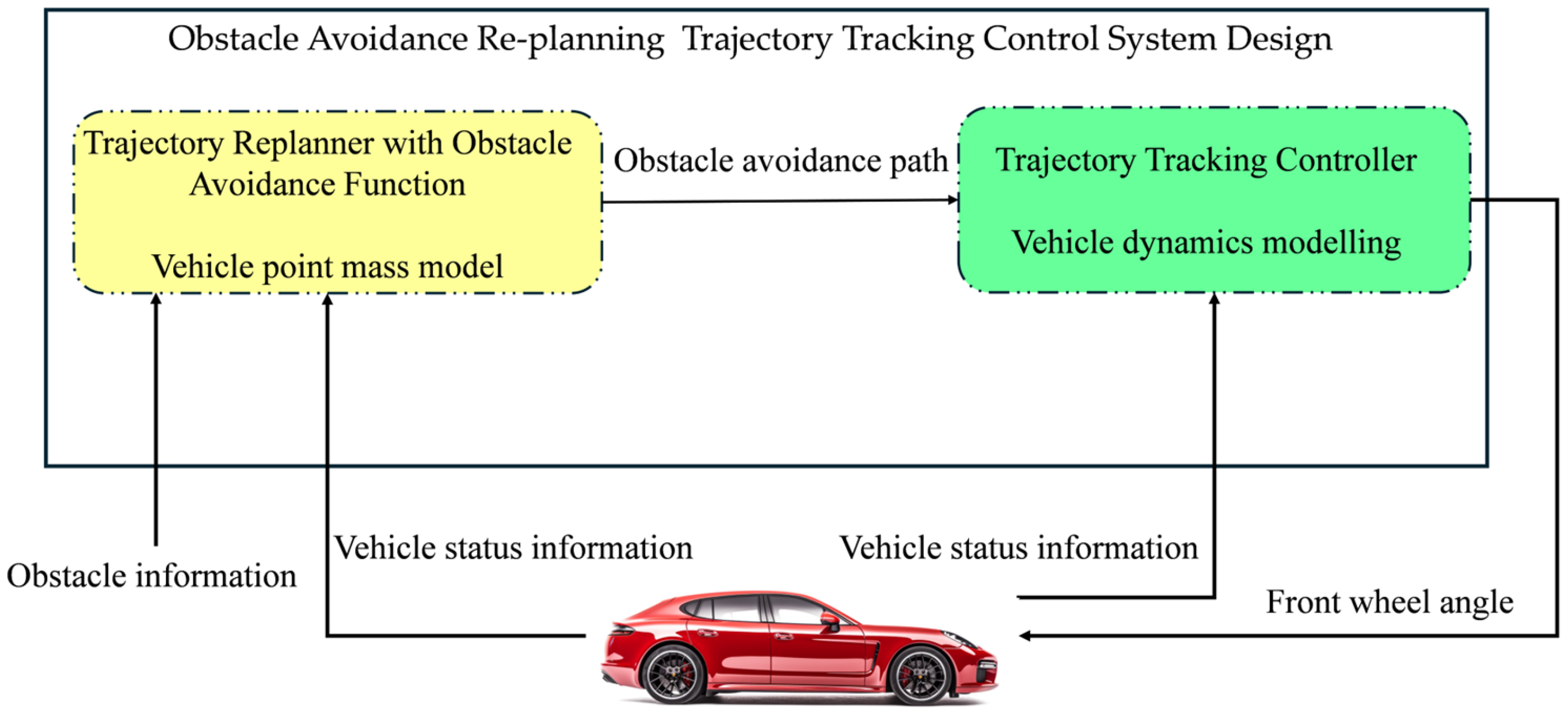
2.1. Obstacle Avoidance Re-Planning Trajectory-Tracking Control System Design

When an intelligent vehicle is driving autonomously on a real road, the presence of pedestrians, other vehicles, and obstacles makes the environment around the vehicle very complex, so the vehicle may not be able to ensure the safety of the vehicle just by direct tracking of the reference trajectory [15,16]. When there are obstacles in the reference trajectory, it creates an obstacle avoidance trajectory-tracking problem, and the intelligent vehicle needs to safely avoid obstacles under the premise of satisfying the problem’s constraints and then fit the reference trajectory as much as possible to complete the trajectory tracking.

This paper designs a trajectory-tracking control system with obstacle avoidance, as shown in Figure 1. This control system is mainly composed of two parts: the obstacle avoidance re-planning controller and the trajectory-tracking controller. The obstacle avoidance re-planning controller uses the obstacle information identified by the sensing module and the reference trajectory information to plan a temporary trajectory that can avoid obstacles, and outputs it to the trajectory-tracking controller. The trajectory-tracking controller calculates and analyses the corresponding front wheel rotation angle according to the temporary trajectory, and transmits this information to the intelligent vehicle to complete the tracking control action for the obstacle avoidance trajectory.

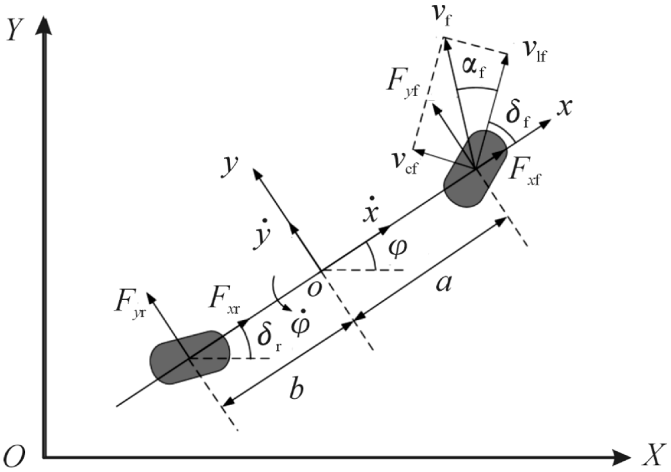
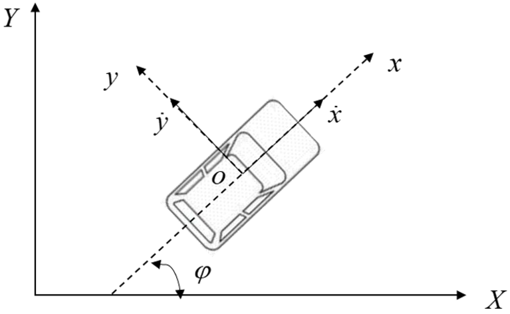
2.2. Modelling of Vehicle Dynamics

Vehicle modelling is the basis for studying intelligent vehicles to realize trajectory planning and trajectory-tracking control, and it needs to be simplified as much as possible due to the need for accurate descriptions of dynamics in order to reduce the computational demands of control algorithms [17]. Figure 2 shows the three-degrees-of-freedom vehicle monorail model.

According to Newton’s second law, the force balance equation is as follows:

$$\left\{\begin{array}{c}m\ddot{x}=m\dot{y}\dot{\phi }+2{{\displaystyle F}}_{x\mathrm{f}}+2{{\displaystyle F}}_{x\mathrm{r}}\\ m\ddot{y}=-m\dot{y}\dot{\phi }+2{{\displaystyle F}}_{y\mathrm{f}}+2{{\displaystyle F}}_{y\mathrm{r}}\\ {{\displaystyle I}}_z\ddot{\phi }=2a{{\displaystyle F}}_{y\mathrm{f}}-2b{{\displaystyle F}}_{y\mathrm{r}}\end{array}\right.$$

(1)

The variables in this equation include m, representing the mass of the vehicle; $a$ and $b$, denoting the distance from the centre mass of the vehicle to the front and rear axes, respectively; $I_z$, which is the moment of inertia around the Z-axis; $F_{x\mathrm{f}}$ and $F_{x\mathrm{r}}$, representing the X-axis directional force on the front and rear wheels of the vehicle, respectively; and $F_{y\mathrm{f}}$ and $F_{y\mathrm{r}}$, denoting the Y-axis directional force on the front and rear wheels, respectively.

In accordance with the established relationship between the body coordinate system and the ground inertia coordinate system, the following formula can be deduced:

$$\left\{\begin{array}{l}\dot{Y}=\dot{x}\sin \phi +\dot{y}\cos \phi \\ \dot{X}=\dot{x}\cos \phi -\dot{y}\sin \phi \end{array}\right.$$

(2)

According to the tire force [18], when combined with Equations (1) and (2), the vehicle dynamics model can be obtained as follows:

$$\left\{\begin{array}{l}\ddot{x}=\dot{y}\dot{\phi }+{\displaystyle \frac{2}{m}}\left[{{\displaystyle C}}_{\mathrm{lf}}{{\displaystyle s}}_{\mathrm{f}}-{{\displaystyle C}}_{\mathrm{cf}}\left({{\displaystyle \delta }}_{\mathrm{f}}-{\displaystyle \frac{\dot{y}+a\dot{\phi }}{\dot{x}}}\right){{\displaystyle \delta }}_{\mathrm{f}}+{{\displaystyle C}}_{\mathrm{lr}}{{\displaystyle s}}_{\mathrm{r}}\right]\\ \ddot{y}=-\dot{x}\dot{\phi }+{\displaystyle \frac{2}{m}}\left[{{\displaystyle C}}_{\mathrm{cf}}\left({{\displaystyle \delta }}_{\mathrm{f}}-{\displaystyle \frac{\dot{y}+a\dot{\phi }}{\dot{x}}}\right)+{{\displaystyle C}}_{\mathrm{cr}}{\displaystyle \frac{b\dot{\phi }-\dot{y}}{\dot{x}}}\right]\\ \ddot{\phi }={\displaystyle \frac{2}{{{\displaystyle I}}_z}}\left[a{{\displaystyle C}}_{\mathrm{cf}}\left({{\displaystyle \delta }}_{\mathrm{f}}-{\displaystyle \frac{\dot{y}+a\dot{\phi }}{\dot{x}}}\right)-b{{\displaystyle C}}_{\mathrm{cr}}{\displaystyle \frac{b\dot{\phi }-\dot{y}}{\dot{x}}}\right]\end{array}\right.$$

(3)

The following variables must be considered: $C_{\mathrm{l}\mathrm{f}}$ and $C_{\mathrm{l}\mathrm{r}}$ are the longitudinal stiffness of the front and rear wheels, respectively; $s_{\mathrm{f}}$ and $s_{\mathrm{r}}$ are the slip rates of the front and rear wheels, respectively; $C_{\mathrm{c}\mathrm{f}}$ and $C_{\mathrm{c}\mathrm{r}}$ are the lateral deflection stiffnesses of the front and rear wheels, respectively; and ${\delta }_{\mathrm{f}}$ and ${\delta }_{\mathrm{r}}$ are the turning angles of the front and rear wheels, respectively.

2.3. Obstacle Avoidance Trajectory Re-Planning Controller Design

2.3.1. Predictive Model

The planning module cycle is generally longer than the control cycle; in order to reduce the computation of the planning module and improve the system response between the planning module and the control module, this chapter adopts a point mass model with good real-time performance as the prediction model for the planning module, which will ignore the body dimensions and does not take into account the load transfer that occurs during the motion process, and only uses a mass model to describe the vehicle’s motion state, which is simpler than either the vehicle kinematic model or the vehicle dynamics model, and its biggest advantage is that it can take a vehicle’s lateral acceleration constraints into account. The vehicle point mass model is shown below:

The point mass model is built in in the geodetic coordinate system XOY and the body coordinate system xoy. In Figure 3, $\dot{x}$ and $\dot{y}$ are the longitudinal and transverse velocities of the vehicle in the body coordinate system, respectively. Assuming that the vehicle is travelling at a constant speed, the expressions of the kinematic equations for the point mass of the vehicle are as follows:

$$\left\{\begin{array}{l}\ddot{y}={{\displaystyle a}}_y\\ \ddot{x}=0\\ \dot{\phi }={\displaystyle \frac{{{\displaystyle a}}_y}{\dot{x}}}\\ \dot{Y}=\dot{x}\sin \phi +\dot{y}\cos \phi \\ \dot{X}=\dot{x}\cos \phi -\dot{y}\sin \phi \end{array}\right.$$

(4)

In the formula, $\dot{Y}$ and $\dot{X}$ are the longitudinal and transverse velocities of the vehicle in the geodetic coordinate system, respectively; $a_y$ is the longitudinal accelerations of the vehicle, respectively; and $\phi$ and $\dot{\phi }$ are the transverse swing angle and transverse swing angular velocity of the vehicle, respectively.

Using the above state space equations as a predictive model for the system, the nonlinear system is expressed as follows:

$$\left\{\begin{array}{l}\dot{\xi }\left(t\right)=f\left(\xi \left(t\right),u\left(t\right)\right)\\ \eta \left(t\right)=C\xi \left(t\right)\end{array}\right.$$

(5)

In the formula, the state quantity $\xi ={\left[\dot{y} \dot{x} \phi Y X\right]}^T$, the control quantity $u=\left[a_y\right]$, and the output quantity matrix $C=\left[\begin{array}{ccccc}0& 0& 1& 0& 0\\ 0& 0& 0& 1& 0\end{array}\right]$.

The system is obtained by discretising the system using zero-order system keeping:

$$\xi \left(k+i+1\right)=\xi \left(k+i\right)+\Delta Tf\left(\xi \left(k+i\right),u\left(k+i\right)\right), i=0, 1, \cdots , {{\displaystyle N}}_p-1$$

(6)

The optimal control quantity for the above nonlinear model predictive control is $\mathrm{U}$, which is defined in the following form:

$$U\left(k\right)=\left[\begin{array}{l}u\left(k\left|k\right.\right)\\ u\left(k+1\left|k\right.\right)\\ ⋮\\ u\left(k+{{\displaystyle N}}_c-1\left|k\right.\right)\end{array}\right]$$

(7)

According to Formulas (6) and (7), the state quantities of the system in the whole prediction time domain can be introduced, and the specific derivation process is as follows:

$$\begin{array}{l}\xi \left(k+1\right)=\xi \left(k\left|k\right.\right)+\Delta Tf\left(\xi \left(k\left|k\right.\right),u\left(k\left|k\right.\right)\right)\\ \xi \left(k+2\right)=\xi \left(k+1\left|k\right.\right)+\Delta Tf\left(\xi \left(k+1\left|k\right.\right),u\left(k+1\left|k\right.\right)\right)\\ ⋮\\ \xi \left(k+{{\displaystyle N}}_c\right)=\xi \left(k+{{\displaystyle N}}_c-1\left|k\right.\right)+\Delta Tf\left(\xi \left(k+{{\displaystyle N}}_c-1\left|k\right.\right),u\left(k+{{\displaystyle N}}_c-1\left|k\right.\right)\right)\\ ⋮\\ \xi \left(k+{{\displaystyle N}}_p\right)=\xi \left(k+{{\displaystyle N}}_p-1\left|k\right.\right)+\Delta Tf\left(\xi \left(k+{{\displaystyle N}}_p-1\left|k\right.\right),u\left(k+{{\displaystyle N}}_c-1\left|k\right.\right)\right)\end{array}$$

(8)

Consequently, the subsequent equation for the system’s output in the prediction time domain can be deduced on the basis of the relationship between the system’s output and the state quantities.

$$\begin{array}{ll}\eta \left(k+1\left|k\right.\right)& =C\xi \left(k+1\left|k\right.\right)\hfill \\ & =C\xi \left(k\left|k\right.\right)+C\Delta \Delta T\left(\xi \left(k\left|k\right.\right),u\left(k\left|k\right.\right)\right)\hfill \\ \eta \left(k+2\left|k\right.\right)& =C\xi \left(k+2\left|k\right.\right)\hfill \\ & =C\xi \left(k+1\left|k\right.\right)+C\Delta \Delta T\left(\xi \left(k+1\left|k\right.\right),u\left(k+1\left|k\right.\right)\right)\hfill \\ ⋮\hfill \\ \hfill \eta \left(k+{{\displaystyle N}}_c\left|k\right.\right)& =C\xi \left(k+{{\displaystyle N}}_c\right)\hfill \\ & =C\xi \left(k+{{\displaystyle N}}_c-1\left|k\right.\right)+C\Delta \Delta T\left(\xi \left(k+{{\displaystyle N}}_c-1\left|k\right.\right),u\left(k+{{\displaystyle N}}_c-1\left|k\right.\right)\right)\hfill \\ ⋮\hfill \\ \eta \left(k+{{\displaystyle N}}_p\left|k\right.\right)\hfill & =C\xi \left(k+{{\displaystyle N}}_p\right)\hfill \\ & =C\xi \left(k+{{\displaystyle N}}_p-1\left|k\right.\right)+C\Delta \Delta T\left(\xi \left(k+{{\displaystyle N}}_p-1\left|k\right.\right),u\left(k+{{\displaystyle N}}_c-1\left|k\right.\right)\right)\hfill \end{array}$$

(9)

At this juncture, it is feasible to obtain the output quantities in the prediction time domain $N_p$ based on the current state quantities of the system and the sequence of control quantities in the future control time domain $N_c$, which in turn completes the iteration.

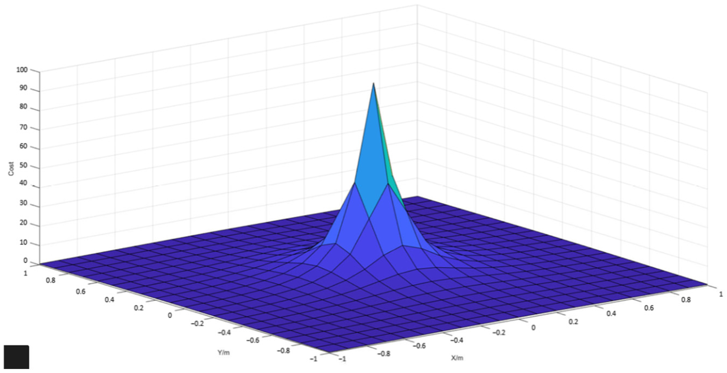
2.3.2. Obstacle Avoidance Function and Objective Function Design

The function of the obstacle avoidance controller is to plan an obstacle avoidance trajectory that meets a set of requirements based on obstacle information. In the process of an intelligent vehicle travelling, obstacle information is generally recognized and perceived by a sensor system equipped on the intelligent vehicle. When obstacle points are close to each other, they can be directly interpreted as a large obstacle to be processed; when obstacle points are distant from each other, they can be directly interpreted as a number of individual small obstacles. Therefore, selection in the obstacle avoidance function needs to take into account the specific location information of the obstacles. There also exists a penalty function, in order to is to adjust function value by calculating the deviation of the distance between the vehicle and the obstacle [19]. In this paper, the selected obstacle avoidance function is as follows:

$$\left\{\begin{array}{l}{{\displaystyle J}}_{obs,i}={\displaystyle \frac{{{\displaystyle S}}_{obs}{{\displaystyle v}}_i}{{{\displaystyle \left({{\displaystyle x}}_i-{{\displaystyle x}}_0\right)}}^2+{{\displaystyle \left({{\displaystyle y}}_i-{{\displaystyle y}}_0\right)}}^2+\epsilon }}\\ {{\displaystyle v}}_i={{\displaystyle v}}_x^2+{{\displaystyle v}}_y^2\end{array}\right.$$

(10)

In the formula, $S_{obs}$ is the weighting factor, $(x_i,y_i)$ is the positional coordinates of the obstacle in the body coordinate system, $(x_0,y_0)$ is the vehicle centre of mass coordinates, and $\epsilon$ is a smaller positive number to prevent the denominator from being zero.

A schematic diagram of the obstacle avoidance function is shown in Figure 4. When the obstacle is far away from the vehicle, the value of the obstacle avoidance function is small, as shown in the dark blue region of the figure; when the obstacle is closer to the vehicle, the value of the obstacle avoidance function increases, as shown in the light blue region of the figure.

Firstly, the heading angle of the vehicle should be consistent with the centre line of the lane during normal driving; secondly, all obstacles can be avoided safely when encountering obstacles; and finally, the steering frequency and amplitude of the vehicle should be considered to ensure the comfort and safety of the ride. Based on the above three objectives, the design objective function is as follows [18]:

$$\begin{array}{l}\underset{{{\displaystyle u}}_t}{\min }{\displaystyle \sum _{i=1}^{{{\displaystyle N}}_p}{{\displaystyle ‖\phi \left(k+i\left|k\right.\right)-{{\displaystyle \phi }}_{ref}\left(k+i\left|k\right.\right)‖}}_Q^2+{\displaystyle \sum _{i=0}^{{{\displaystyle N}}_c-1}{{\displaystyle ‖u\left(k+i\left|k\right.\right)‖}}_R^2}}+{{\displaystyle J}}_{obs,i}\\ s.t.{{\displaystyle X}}_{\min }<X(k+i)<{{\displaystyle X}}_{\max }\hfill \\ \hspace{1em} {{\displaystyle {{\displaystyle a}}_y}}_{\min }<{{\displaystyle a}}_y\left(k+i\right)<{{\displaystyle {{\displaystyle a}}_y}}_{\max }\hfill \end{array}$$

(11)

In the formula, the first expression reflects the vehicle’s need to follow the centre line of the lane to ensure that the vehicle can follow the lane, near the centre line of the lane, after successfully avoiding an obstacle, while the second characterises the magnitude and frequency of the vehicle’s steering angle during obstacle avoidance, to maintain lateral stability when steering to avoid an obstacle. $J_{obs,i}$ is the value of the obstacle avoidance function at sampling moment $i$.

2.3.3. Fifth-Degree Polynomial Fitting of Obstacle Avoidance Trajectories

The planning layer is solved by optimisation to obtain a series of discrete collision-free points; the number of discrete points is related to the length of the prediction time domain, and pN discrete points will be generated in the prediction time domain pN. If the planning layer is directly delivered to the motion control layer in the form of discrete points, it is necessary to change the number of upper and lower controller interfaces simultaneously when different prediction time domains are used, and, secondly, this will also lead to the disadvantage in that the input interfaces will take up too much memory; in addition, due to the inconsistency of the sampling period of the planning layer and the motion control layer, there is a timestamp between the sequence of discrete points in the planning layer and the target points in the motion control layer, and therefore it is necessary to convert these discrete points into continuous curves by curve fitting. Considering that the first-order and second-order derivatives of the quintic polynomial are continuous, which can ensure that the velocity and acceleration of the curve can be well followed by the motion control layer, the quintic polynomial is used to curve-fit the discrete path points, and the expression of the quintic polynomial is as follows:

$$\left\{\begin{array}{l}Y={{\displaystyle a}}_0{{\displaystyle X}}^5+{{\displaystyle a}}_1{{\displaystyle X}}^4+{{\displaystyle a}}_2{{\displaystyle X}}^3+{{\displaystyle a}}_3{{\displaystyle X}}^2+{{\displaystyle a}}_{4}X+{{\displaystyle a}}_5\\ \phi ={{\displaystyle b}}_0{{\displaystyle X}}^5+{{\displaystyle b}}_1{{\displaystyle X}}^4+{{\displaystyle b}}_2{{\displaystyle X}}^3+{{\displaystyle b}}_3{{\displaystyle X}}^2+{{\displaystyle b}}_{4}X+{{\displaystyle b}}_5\end{array}\right.$$

(12)

In the formula, $Y$ is the vehicle position transverse coordinate, $\phi$ is the vehicle’s swing angle, and $a_p=\left[a_0,a_1,a_2,a_3,a_4{,a}_5\right]$ and $b_p=\left[b_0,b_1,b_2,b_3,b_4{,b}_5\right]$ are the coefficients to be determined for the fifth-degree polynomial.

2.4. Adaptive Predictive Time Domain Trajectory Tracker Design

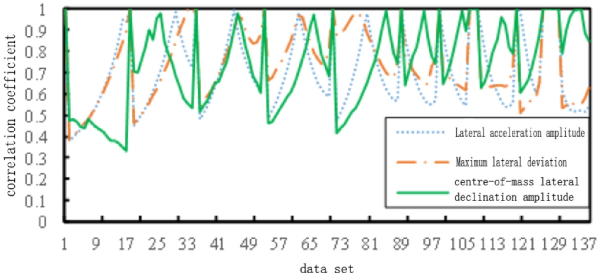
2.4.1. Gray Correlation Analysis

Statistical methods used to carry out systematic analysis of the more classic methods are as follows: regression analysis, analysis of variance, principal component analysis, etc.; these methods tend to be grey, as there is no typical distribution pattern. The core idea of grey correlation analysis is to judge the degree of connection between the characteristic sequences based on the fit of the increasing and decreasing trends of the curves drawn by the parameters of the sequences, and it, in principle, does not require the quality of the samples; additionally, the quantitative results of the analyses using the grey correlation analysis method will always be the same as the results of the qualitative analyses, which is a great natural advantage of the grey correlation analysis method over the other mathematical statistical analysis methods.

The grey correlation reflects the degree of influence of the factors in the system on the target value, and the general steps of analysis using the grey correlation method are as follows:

• Determining the analytical series;

First, two key sets of series are defined: a reference series, reflecting the properties of the system, which consists of data characterising the behaviour of the system, and a comparison series, containing data on the factors influencing the behaviour of the system. Each of these two sets of series provides a quantitative description of the state of the system and the factors influencing it. As further analysed below, the reference series, also known as the parent series, is denoted as: $Y=\left\{Y\left(k\right)\left|k=1,2,\wedge ,n\right.\right\}$; the comparison series, also known as the subsequence can be denoted as: $X_i=\left\{X_i\left(k\right)\left|k=1,2,\wedge ,n\right.\right\},i=1,2,\wedge ,m$.

2.

Dimensionlessness of variables;

Dimensionless treatment of variables is carried out to enable data of different magnitudes to be compared under the same criteria, ensuring the accuracy and reliability of analysis results.

$${{\displaystyle x}}_i\left(k\right)={\displaystyle \frac{{{\displaystyle X}}_i\left(k\right)}{{{\displaystyle X}}_i\left(k\right)}}, k=1, 2, \Lambda , n; i=0, 1, 2, \Lambda , m$$

(13)

3.

Calculate the grey correlation coefficient between the parent sequence and the subsequence.

The correlation coefficient between $X_0\left(k\right)$ and $X_i\left(k\right)$ is calculated with the formula:

$${\xi }_i(k)={\displaystyle \frac{\underset{i}{\min } \underset{k}{\min }|y(k)-x_i(k)|+\rho \underset{i}{\max } \underset{k}{\max }|y(k)-x_i(k)|}{|y(k)-x_i(k)|+\rho \underset{i}{\max } \underset{k}{\max }|y(k)-x_i(k)|}}$$

(14)

Making ${∆}_i\left(k\right)=\left|y\left(k\right),x_i\left(k\right)\right|$ yields the following equation:

$${\xi }_i(k)={\displaystyle \frac{\underset{i}{\min } \underset{k}{\min }{\Delta }_i(k)+\rho \underset{i}{\max } \underset{k}{\max }{\Delta }_i(k)}{{\Delta }_i(k)+\rho \underset{i}{\max } \underset{k}{\max }{\Delta }_i(k)}}$$

(15)

In the formula, $\rho$ represents the resolution factor; the larger the $\rho$ value, the smaller the resolving power. The general value of $\rho$ is (0,1), but the value can be adjusted according to the quality of the sample. Usually, ρ is taken to be 0.5.

4.

Calculating correlation;

The correlation coefficient results usually contain multiple dispersed values, and in order to synthesise these moment-specific correlation values into a composite metric, it is necessary to compute an average of these values to obtain a quantitative representation of the overall degree of correlation between the two series [20]. The formula for calculating the degree of association $r_i$ is as follows:

$${{\displaystyle r}}_i={\displaystyle \frac{1}{n}}{\displaystyle \sum _{k=1}^n{{\displaystyle \xi }}_i}\left(k\right), k=1, 2, \Lambda , n$$

(16)

5.

Order by relevance;

If $r_1<r_2$, the reference series $Y$ is more similar to the comparison series $X$. After calculating the correlation coefficients between the $X_i\left(k\right)$ sequence and the $Y\left(k\right)$ sequence, the correlation values can be sorted, and the average $r_i$ of the correlation coefficients for each category, i.e., the correlation between $X_i\left(k\right)$ and $Y\left(k\right)$, can be calculated.

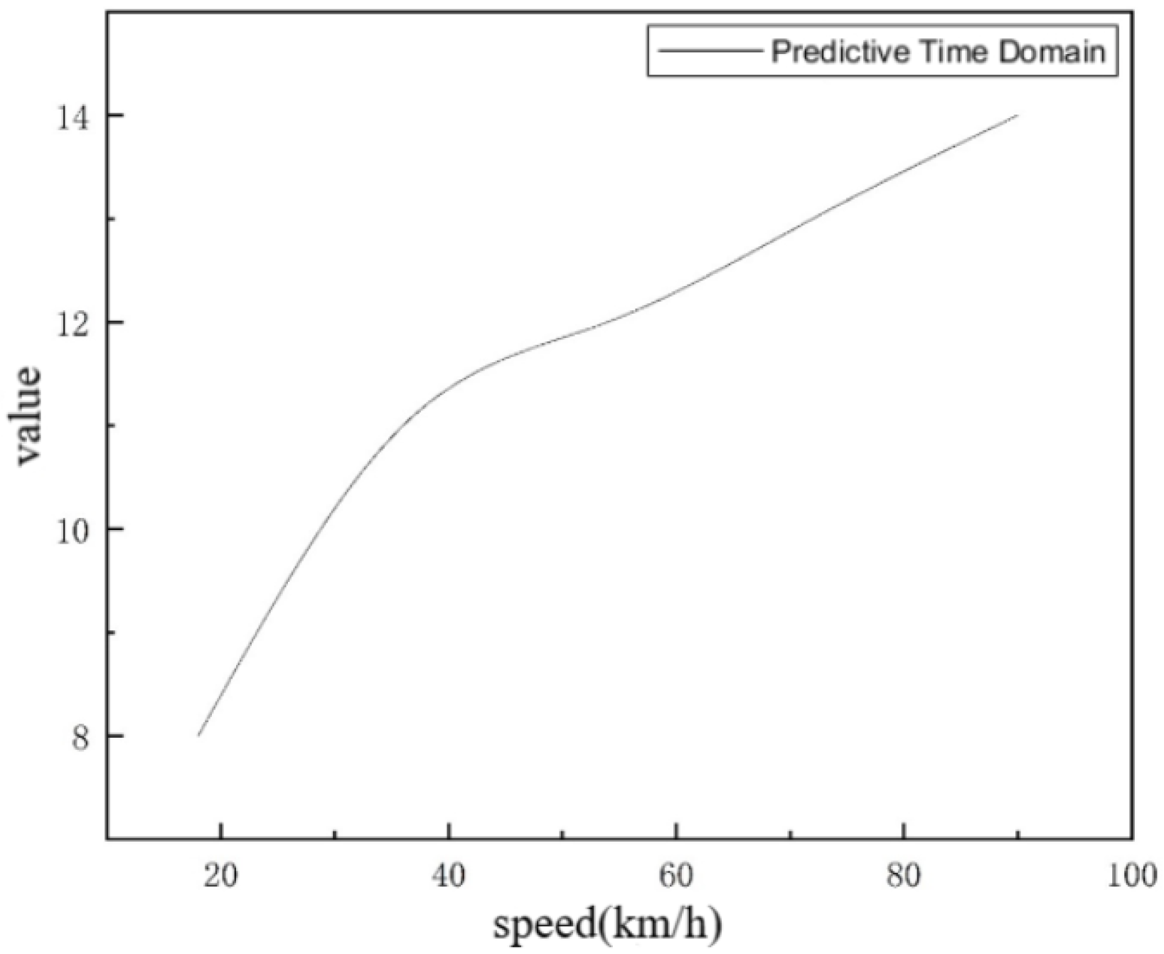
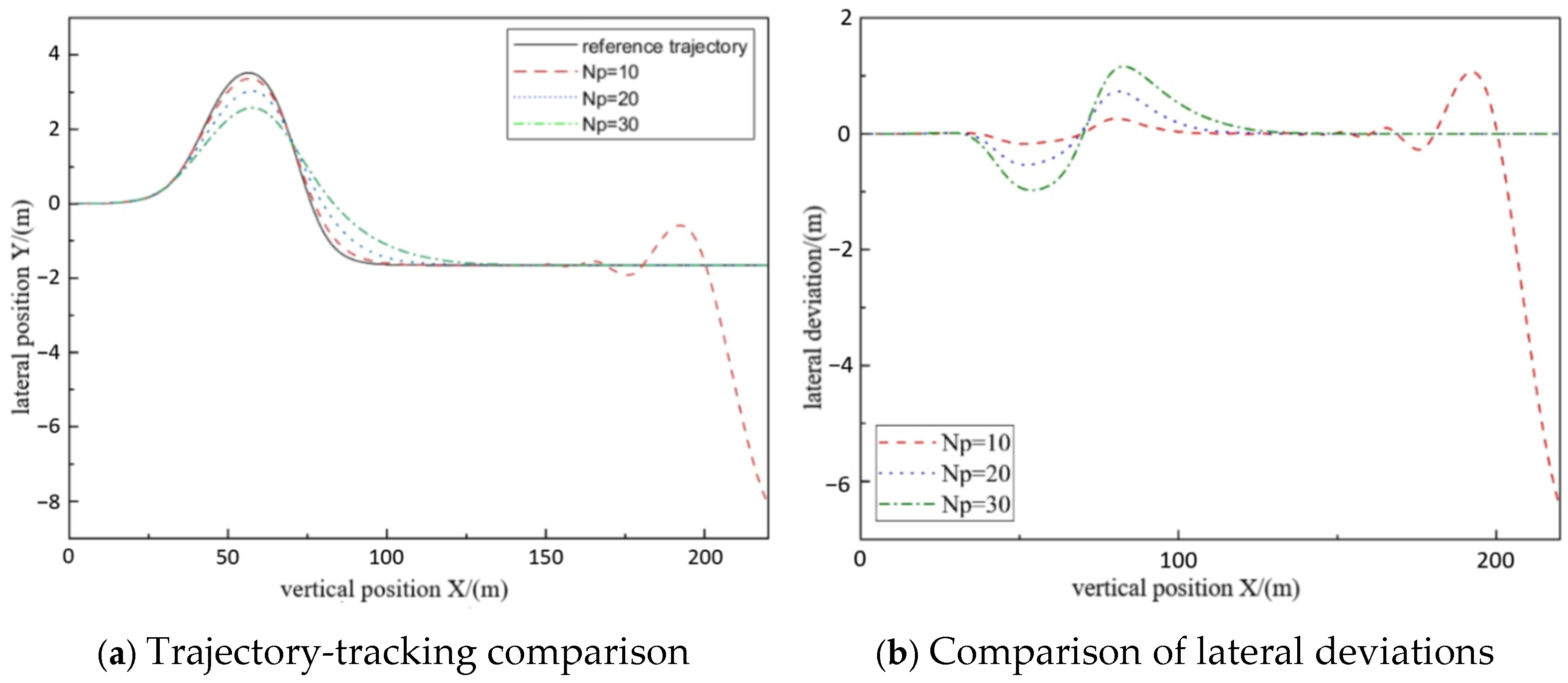
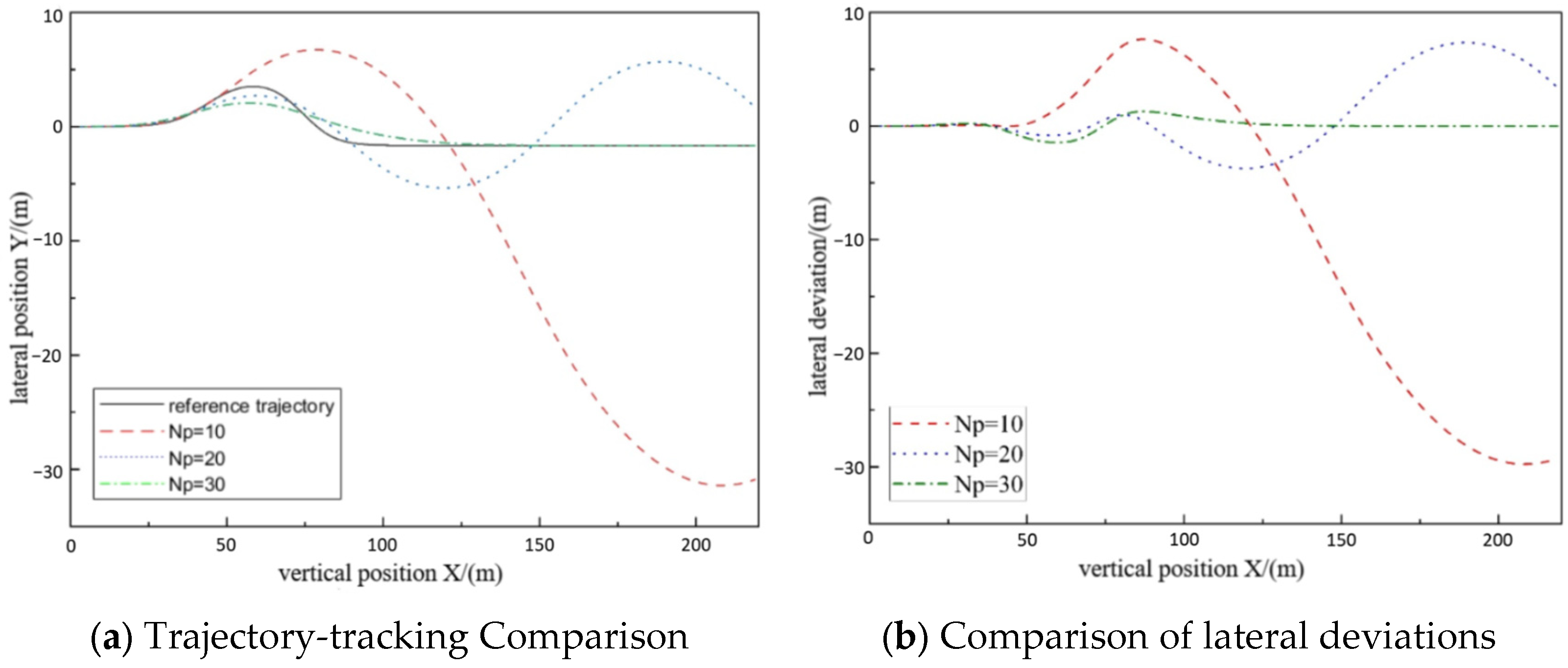
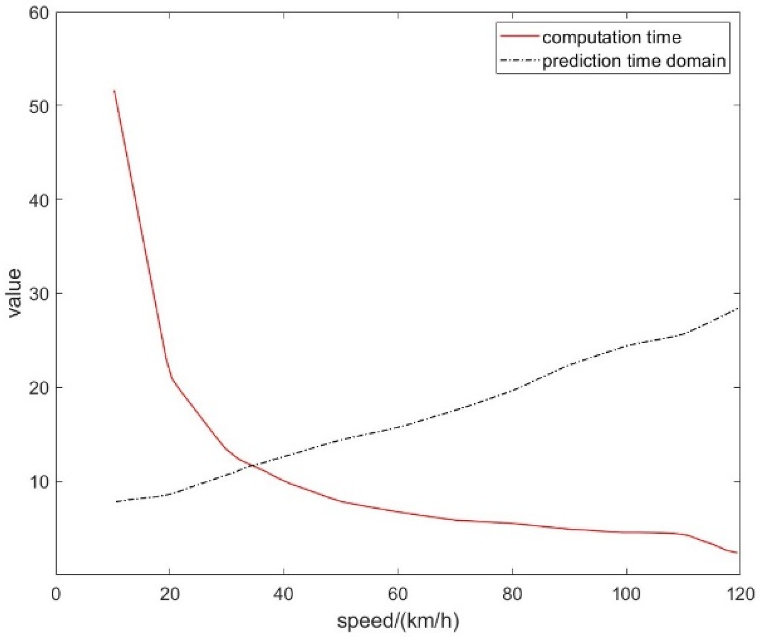
2.4.2. Determination of Optimal Time-Domain Parameters

According to the grey correlation analysis method, the predicted time-domain parameter $N_p$ is selected as the parent sequence, and the maximum lateral deviation of the reprogrammed trajectory from the reference trajectory, the lateral acceleration amplitude, and the amplitude of the lateral deviation of the centre of mass are used as the characteristic sequences (evaluation items) to analyse the degree of correlation of each evaluation item to the parent sequence. The maximum lateral deviation reflects the error between the reprogrammed trajectory and the original reference trajectory, and the lateral acceleration amplitude and the centre-of-mass lateral declination amplitude reflect the stability of the vehicle motion and ride comfort during the tracking process.

In the environment where the reference trajectory is set as a lane-changing double-shifted line trajectory and there are multiple obstacles, 5 m/s is used as the speed interval, and offline simulation experiments are carried out for the controller within a speed interval from 18 to 90 km/h. The value range of the prediction time domain is set to [5,15] with reference to the simulation experience, and the total number of experimental groups is 300. To ensure the effectiveness of the controller’s prediction time-domain parameters, the parameters are selected based on the following criteria:

• The selected time-domain parameters should enable the trajectory re-planning process to smoothly avoid obstacles;
• The selected time-domain parameters should result in a new trajectory, obtained after re-planning by the controller, having the smallest deviation from the original reference trajectory;
• The selected time-domain parameters should enable the vehicle to re-track the original reference trajectory after obstacle avoidance actions;
• The selected time-domain parameters should not cause overshooting during the tracking test;
• The selected time-domain parameters should not cause yaw angle oscillation during the tracking test.

Based on the above screening conditions, 138 groups of tests satisfying the requirements were obtained. In order to facilitate the integration of the index data into the scale, the evaluation items with smaller values were multiplied by 10, and the resolution coefficient was taken as 0.5, so that the correlation coefficients between the parent series prediction time domain parameter Np and the evaluation items of each sub-sequence were obtained as shown in Figure 5.

The grey correlation of each evaluation item to $N_p$ was calculated according to Equation (16):

$${{\displaystyle r}}_n={\displaystyle \sum _{i=1}^{138}{{\displaystyle \tilde{\omega }}}_i}{{\displaystyle \xi }}_{{{\displaystyle N}}_{p,c}}\left(i\right), n=1, 2, 3$$

(17)

In the formula, $r_n$ represents the grey relational degree of each evaluation criterion with respect to the time-domain parameters; $\widetilde{{\omega }_i}$ denotes the weight of the $i$-th indicator variable, with equal weights assigned as 1/138 in this context; ${\zeta }_{N_{p,c}}$ represents the domain correlation coefficient for the time domain parameter.

The grey correlation ranking results obtained according to Equation (17) are shown in

Table 1. Gray correlation rankings.

Evaluation Item	Main Sequence	Relevance	Rank
Maximum Lateral Deviation	$N_p$	0.776	1
Lateral Acceleration Amplitude	$N_p$	0.714	2
Centroid Lateral Deviation Amplitude	$N_p$	0.679	3

.

The time-domain grey correlation results show that the maximum lateral deviation has the highest correlation with the predicted time domain, so the minimum value of the maximum bias deviation is used as a reference term in the offline experimental data to select the optimal data set for the predicted time domain at different vehicle speeds.

The Fourier series consists of a series of sums of trigonometric functions, which can be used to fit a continuous periodic function or a periodic function that contains the first type of discontinuity [21]. Because of the periodicity presented by the time-domain parameters with the speed change, this paper uses the Fourier approximation method to fit the time-domain parameters and the speed parameters. The formulae for the Fourier approximation method of fitting are as follows:

$$f(t)={\displaystyle \frac{a_0}{2}}+{\displaystyle \sum _{n=1}^{\infty }}[a_{n}cos(n\omega t)+b_{n}sin(n\omega t)]$$

(18)

In the Formula (19):

$$a_0={\displaystyle \frac{2}{T}}{\int }_{t_0}^{t_0+T}f(t)cos(\omega t)dt, a_n={\displaystyle \frac{2}{T}}{\int }_{t_0}^{t_0+T}f(t)cos(n\omega t)dt,{ b}_n={\displaystyle \frac{2}{T}}{\int }_{t_0}^{t_0+T}f(t)sin(n\omega t)dt$$

(19)

$f\left(t\right)$ is the fitted function; ${\displaystyle \frac{a_0}{2}}$ is the average height of the curve that defines the datum of the fitted curve. $t_0\to t_0+T$ denotes a period; $\omega$ denotes the rotational speed such that the period of the orthogonal function group sin, cos at $n=1$ is the same as the fitted period, so there is $\omega ={\displaystyle \frac{2\pi }{T}}$; $T$ is the period of the fitted function $f\left(t\right)$, where $T=t_{max}-t_{min}$; i.e., the defined interval of the whole function being fitted is a period; $f\left(t\right)\cos \left(n\omega t\right) \mathrm{a}\mathrm{n}\mathrm{d} f\left(t\right)\sin \left(n\omega t\right)$ are the zoom-in and zoom-out of the set of functions for each period by a factor of $f\left(t\right)$ at the point $t$; $a_1,b_1$ is the multiplicative relationship obtained by averaging the $f\left(t\right)\cos \left(\omega t\right) \mathrm{a}\mathrm{n}\mathrm{d} f\left(t\right)\sin \left(\omega t\right)$ integrations and evaluating the group of functions as a whole.

The Fourier approximation method is used to fit the prediction time-domain parameters and speed parameters, and, at the same time, in order to prevent overfitting, the simulation computation time is used as the weight, and, finally, the adaptive prediction time-domain parameter model based on the speed change is obtained as shown in Formula (20), and the prediction time-domain fitting diagram selected after comprehensive evaluation is shown in Figure 6.

$${{\displaystyle N}}_p={\displaystyle \sum _{i=1}^2{{\displaystyle a}}_0}+{{\displaystyle a}}_i\cos \left(ix\omega \right)+{{\displaystyle b}}_i\sin \left(ix\omega \right), 0\le x\le 100$$

(20)

In the equation, $a,b, \mathrm{a}\mathrm{n}\mathrm{d} \omega$ represent the Fourier fitting coefficients of the time domain, and $x$ represents the longitudinal speed of the vehicle in the global coordinate system.

2.4.3. Trajectory-Tracking Controller Function Design

The vehicle model used for trajectory-tracking control is the dynamics model created using Equation (3). The state variables are $(\dot{Y},\dot{X},\dot{\theta },\theta ,Y,X)$, and the control variable is the front wheel steering angle $\delta$. The specific form of the MPC controller for the tracking control layer is shown in Equation (21) [18].

$$\begin{array}{c}\min {\displaystyle \sum _{i=1}^{N_P}}||\eta (t+i|t)-{\eta }_{ref}(t+i|t)|{|}_Q^2+{\displaystyle \sum _{i=1}^{N_c-1}}\parallel \Delta u(t+1|t){\parallel }_R^2+\rho {\epsilon }^2\\ \begin{array}{c}\mathrm{s}.\mathrm{t}.\Delta U_{min}\le \Delta U_t\le \Delta U_{max}\\ U_{min}\le \mathrm{A}\Delta U_t+U_t\le U_{max}\\ y_{hc,min}\le y_{hc}\le y_{hc,max}\\ y_{sc,min}-\epsilon \le y_{sc}\le y_{sc,max}+\epsilon \\ \epsilon >0\end{array}\end{array}$$

(21)

In the equation, ${\eta }_{ref}=\left[Y_{ref},{\phi }_{ref}\right]$ represents the local reference trajectory; $y_{hc}$ represents the hard constraint output; $y_{sc}$ represents the soft constraint output; $y_{hc,min}$ and $y_{hc,max}$ are the hard constraint limits; and $y_{sc,min}$ and $y_{sc,max}$ are the soft constraint limits.

3. Local Obstacle Avoidance Path Planning and Trajectory Tracking Verification

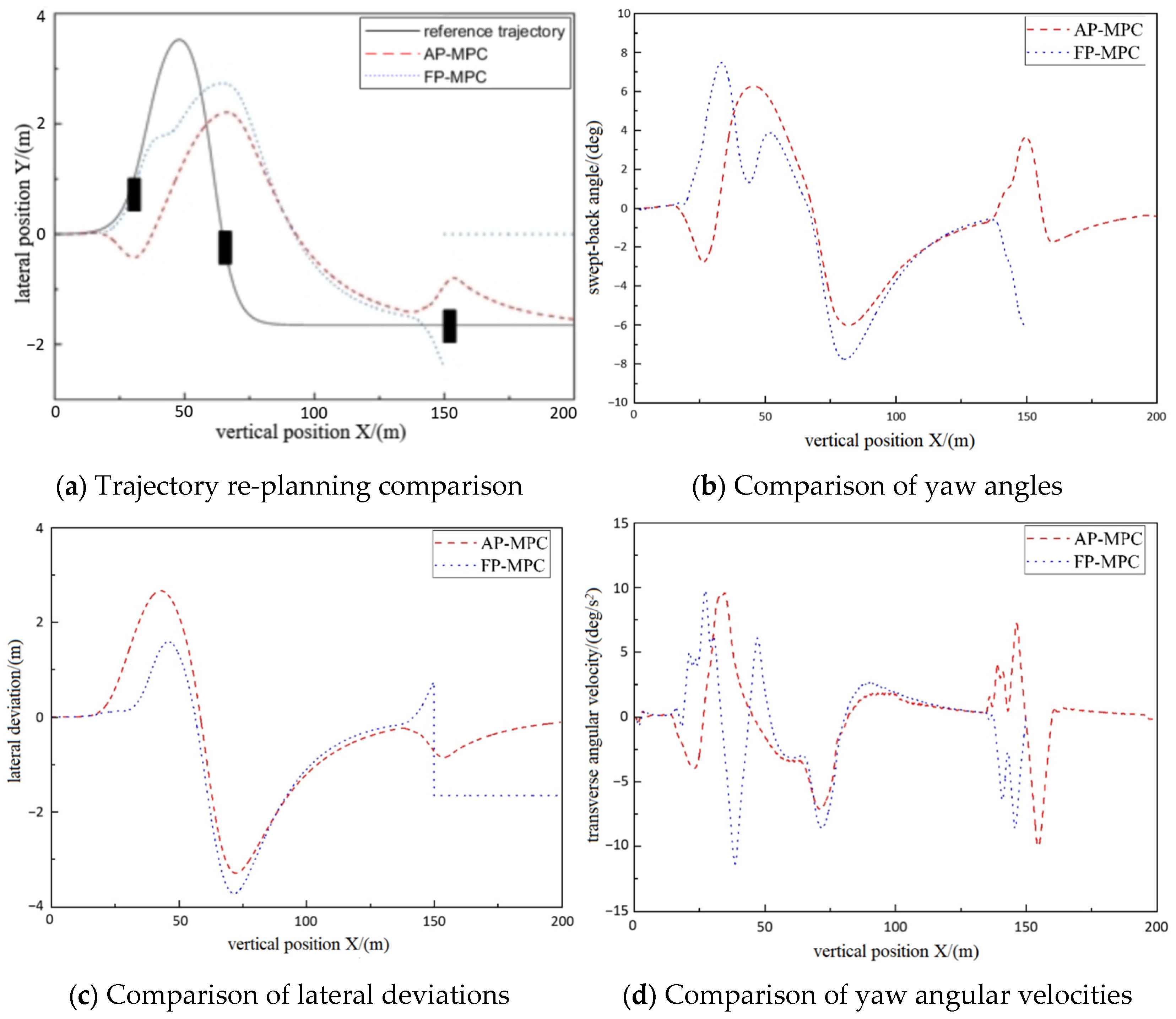
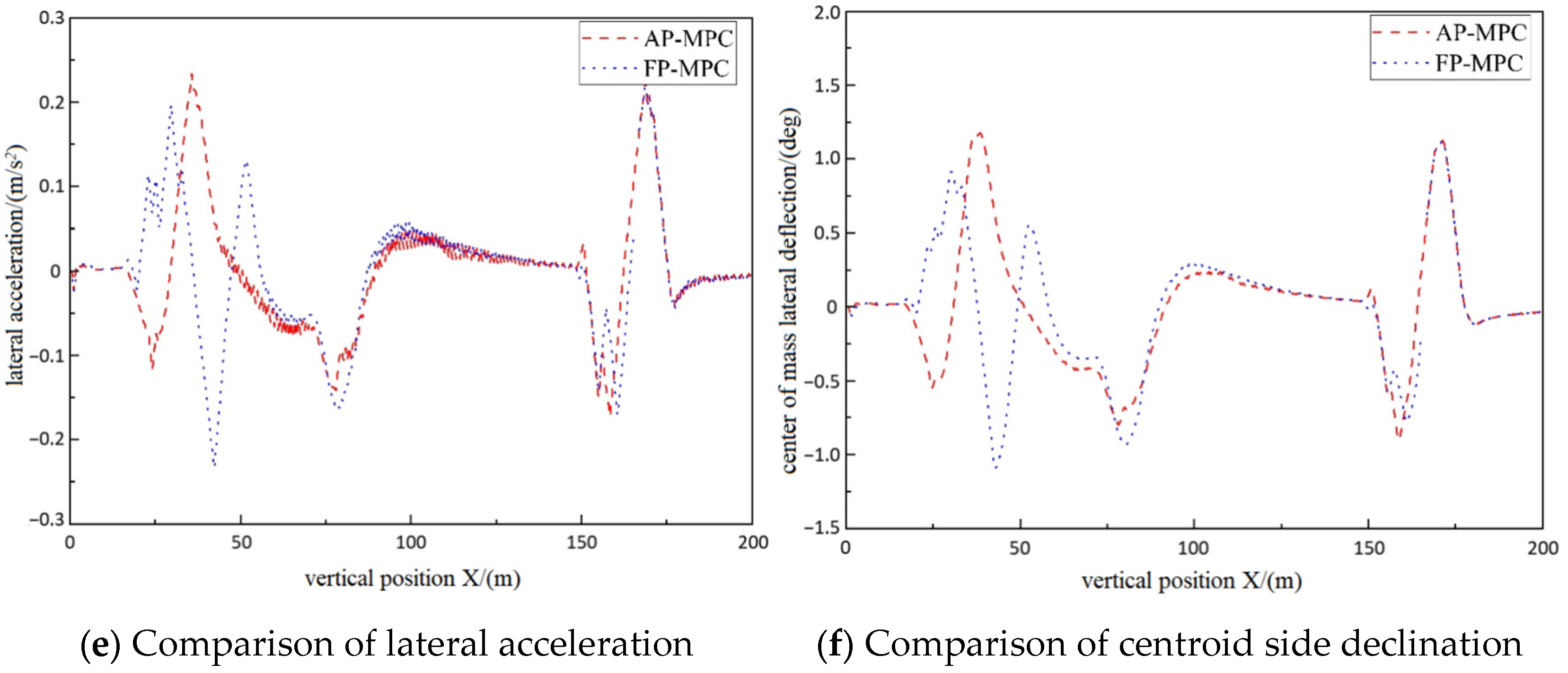
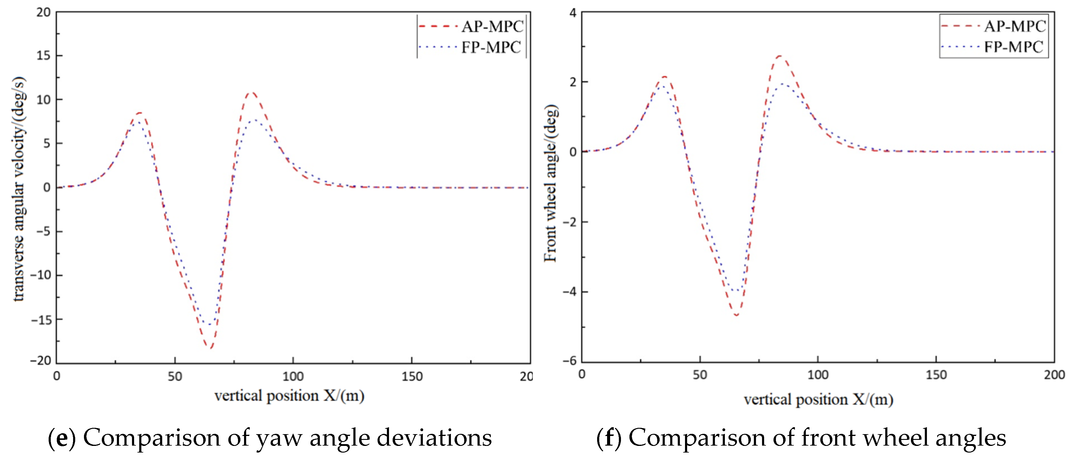
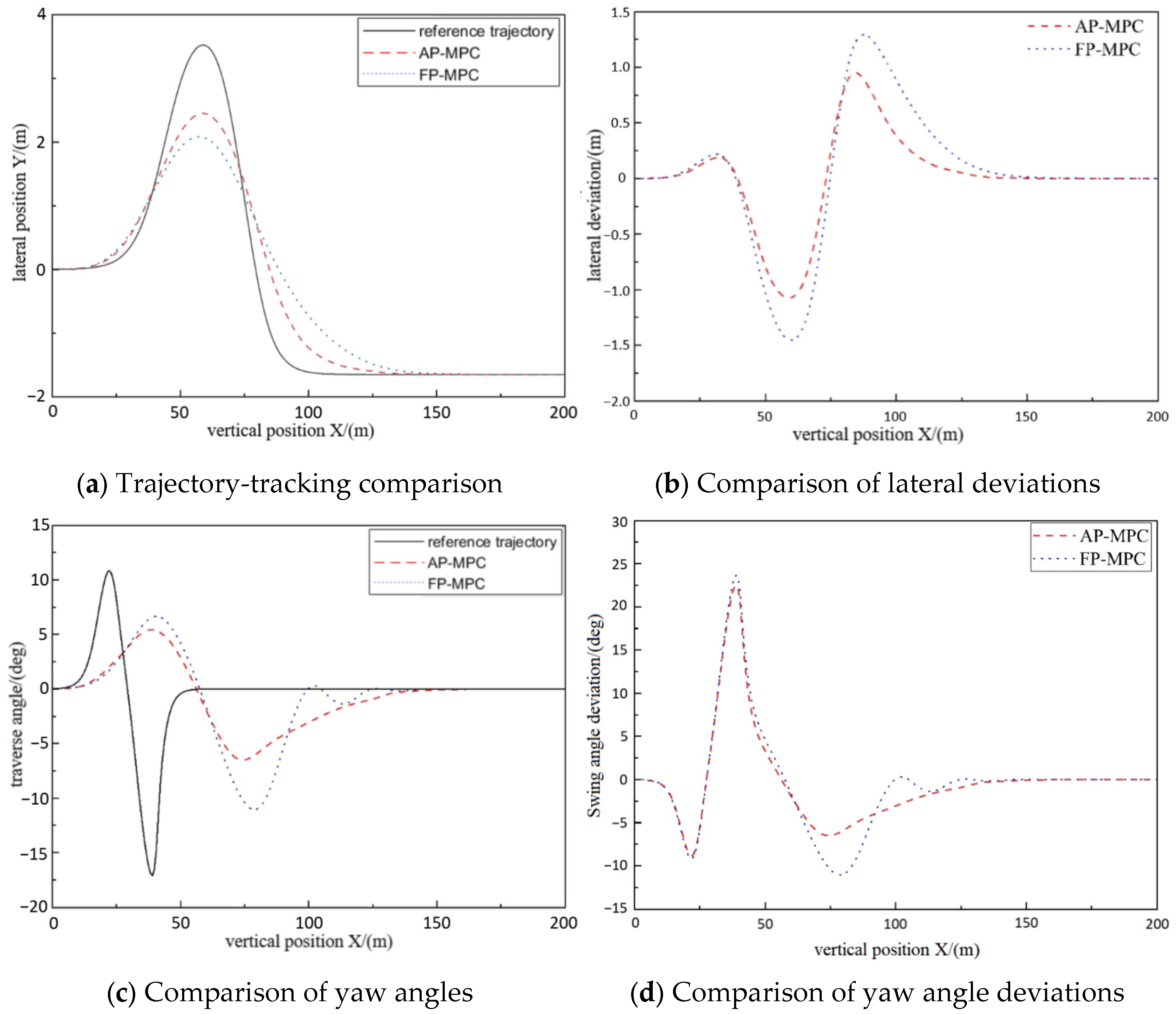
3.1. Comparative Experimental Analysis of Fixed Prediction Time Domain Simulation

To visually demonstrate the impact of different predictive time domains on the trajectory-tracking control process, a MATLAB 2023b/Simulink and CarSim integrated simulation platform was set up for simulation experiment analysis. In CarSim, an E-class vehicle with a wheelbase of 3050 mm was selected as the controlled vehicle model, with basic vehicle parameters listed in

Table 2. Basic vehicle parameters.

Parameter	Value
Vehicle mass, m/kg	1650
Distance from rear axle to vehicle centre of mass, b/m	1.65
Moment of inertia around Z-axis, $I_z/(\mathrm{k}\mathrm{g}·{\mathrm{m}}^2)$	3234
Effective rolling radius of tire, $R_e/\mathrm{m}$	0.32
Centre of mass height, $h_{CG}/\mathrm{m}$	0.53
Front and rear wheel slip ratio, $S_{f,r}$	0.2

and MPC controller parameters in

Table 3. Controller parameters.

Parameter	Value
Prediction Time Domain	10, 20, 30
Control Time Domain	3
Sampling Period, t/s	0.03
Front Wheel Angle Restraint	−10~10°
Front Wheel Angle Increment	$0.53°$
$Q$	$\left[\begin{array}{cc}100& 0\\ 0& 100\end{array}\right]$
$R$	$\left[10\right]$
$\mathrm{Weighting} \mathrm{Factor} \rho$	$1000$

. Simulations were conducted at representative speeds of 50 km/h and 100 km/h, using three sets of different predictive time-domain values for testing on a lane-changing, double lane-change trajectory. The simulation test results are shown in Figure 7 and Figure 8.

From Figure 7, it can be observed that different prediction time domains have varying effects on the controller’s trajectory-tracking performance. When the prediction time domain parameter is set to 10, the controller exhibits minimal lateral deviation while tracking the double lane-change trajectory. However, it shows significant overshoot when tracking straight trajectories, with lateral deviation gradually increasing to 6.5 m, completely deviating from the target trajectory and heading. When the prediction time domain parameter is set to 30, the controller is able to complete the tracking task, but compared to when it is set to 20, there is a larger lateral deviation and some lag in tracking. Combining Figure 7 and Figure 8, it can be seen that as the target tracking speed increases from 50 km/h to 100 km/h, when the predicted time-domain parameter is still taken as 10, the vehicle shows a large offset at the large curvature of the reference trajectory, which indicates that the tracking effect of the FP-MPC controller in complex road conditions has a strong correlation with the change of the vehicle speed under different speed conditions.

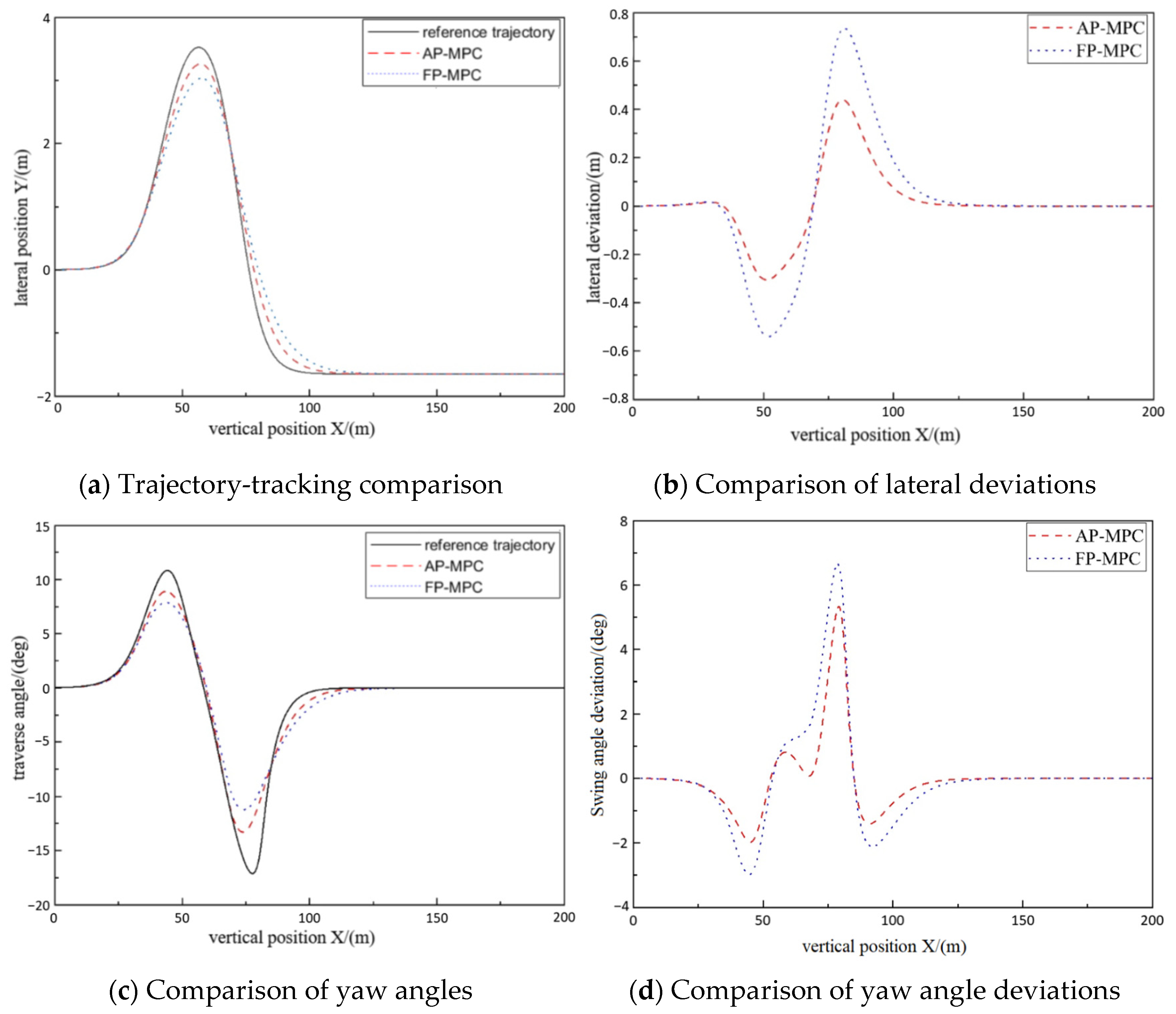
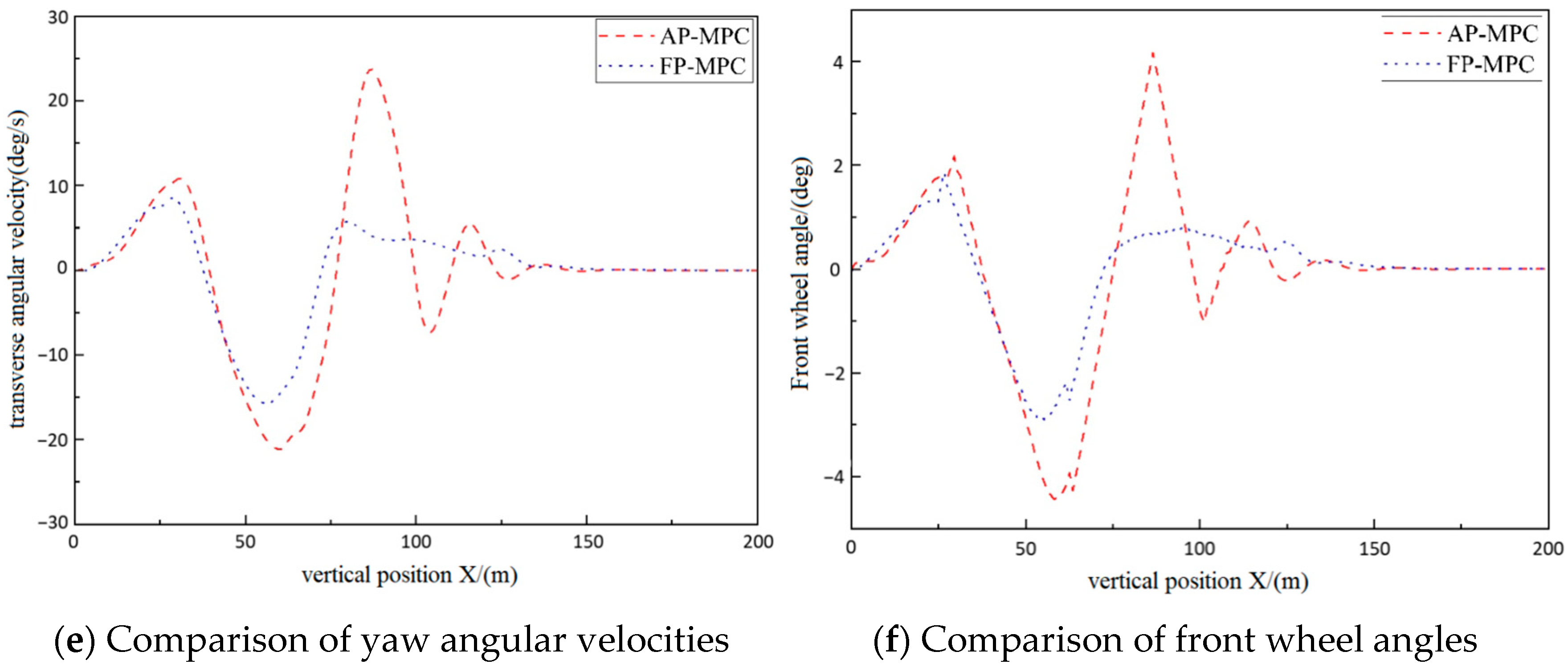
3.2. Simulation Comparison Experiment of AP-MPC

The essence of the adaptive prediction time domain parameter model in Equation (20) is to reduce the computational burden of the algorithm while ensuring controller-tracking accuracy and stability. By selecting relatively optimal prediction time domain parameters, it aims to lower the computational requirements of the controller’s SOC (System-on-Chip). The designed AP-MPC controller’s variation in time-domain prediction parameters with target vehicle speeds and computation times for the double lane-change trajectory in obstacle-free conditions is depicted in Figure 9.

In order to verify the tracking performance of the AP-MPC controller at the control layer, the simulation results are compared with the fixed prediction time-domain FP-MPC controller under the double-shifted lane-changing trajectory, and 50 km/h and 100 km/h are selected as the representative vehicle speeds. The prediction time-domain parameters computed by the adaptive prediction time-domain model are rounded to 50 km/h: $N_p$ = 14; 100 km/h: $N_p$ = 24. The values of other parameters are kept constant, and the simulation results are shown in Figure 10 and Figure 11.

From Figure 10 and Figure 11, it is easy to see that the trajectory-tracking effect of the AP-MPC controller is better than that of the FP-MPC controller under different speed conditions. When the target speed is 50 km/h, the maximum traverse angle deviation of FP-MPC controller is 6.66°, and the measured simulation computation time is 9.17 s, while the maximum traverse angle deviation of AP-MPC controller is 5.33° and the measured simulation computation time is 7.79 s, which indicates an improvement in the control accuracy of 19.9% and the controller solution speed by 15%, and the maximum traverse deviation, traverse angle deviation, and the maximum traverse angle deviation of AP-MPC controller is 5.33° and the measured simulation computation time is 7.79 s. The control accuracy is improved by 19.9%, and the controller solution speed by 15%. The maximum lateral deviation and the oscillation amplitude of the transverse pendulum angle of the controller are smaller than those of the FP-MPC controller. When the speed reaches 100 km/h, the AP-MPC controller effectively reduces the overshooting amount of the trajectory-tracking control, and its maximum traverse angle deviation and maximum lateral deviation are reduced by 0.5% and 26.9%, respectively, compared with those of the timing-domain controller. This shows that under high-speed driving conditions, the AP-MPC controller has better control effects and higher vehicle stability.

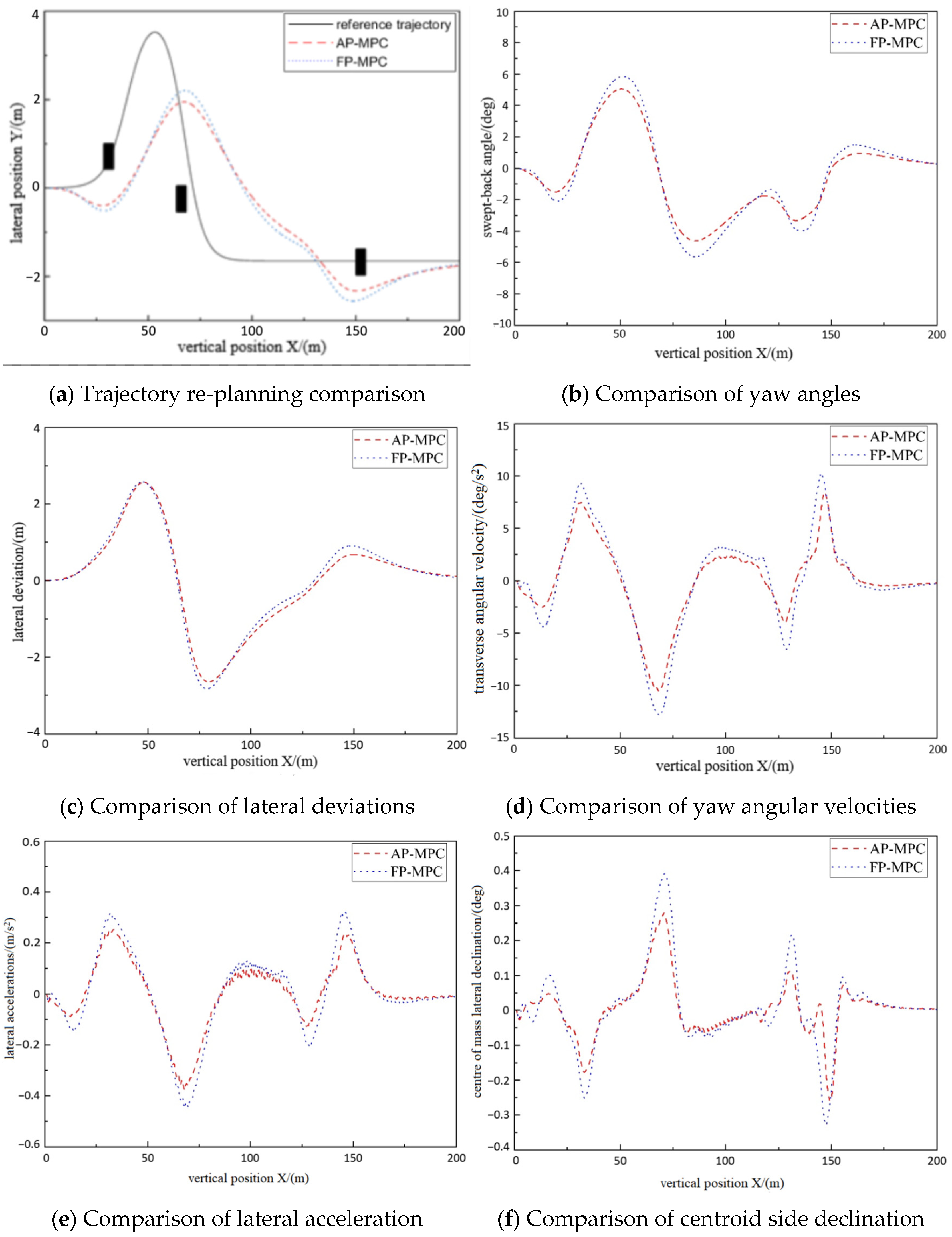
3.3. Comparative Test of AP-MPC Simulation Under Multiple Obstacle Conditions

In the obstacle avoidance re-planning AP-MPC trajectory-tracking simulation experiment, the control time-domain parameters of the tracking controller and the prediction and control time-domain parameters in the planning module are fixed, and the controller prediction time-domain parameters are automatically adjusted by the adaptive prediction time-domain parameter model to study the effect of the change in the prediction time-domain parameters of the control layer, on the trajectory re-planning and tracking control accuracy. The basic parameters of the AP-MPC controller are shown in

Table 4. AP-MPC controller parameters.

Control Parameter	Trajectory Planning Layer	Trajectory-Tracking Layer
Predictive time domain	15	/
Control time domain	2	2
Sampling period T	0.1 s	0.05 s
Front Wheel Angle Restraint	/	$-10°~10°$
Front wheel angle increment	/	0.85°
Weighting matrix Q	$[100]$	$\left[\begin{array}{cc}100& 0\\ 0& 100\end{array}\right]$
Weighting coefficients of the Obstacle avoidance function $S_{obs}$	$500$	/
Weighting matrix R	$[20]$	$5\times {10}^5$
Weighting factor $\rho$	/	1000

.

The joint simulation test ignores the influence of aerodynamics, tire flat ratio, and other factors, as well as the road surface attachment coefficient $\mu$ = 1.0; the reference trajectory is the lane change double-shift line trajectory; the obstacles are set at the first and third large curvature of the trajectory and at the straight-line segment; and the coordinates of the points at the lower left corner of the three obstacles are as follows: obstacle 1: (30, 0.5); obstacle 2: (65, −0.5); obstacle 3: (150, −1.9); the tested vehicles were travelling at the desired speeds of 36 km/h and 72 km/h respectively; according to Equation (20), the values of the prediction time-domain parameters calculated by the adaptive prediction time-domain model after rounding are as follows: 36 km/h:${ N}_p$ = 10; 72 km/h:${ N}_p$ = 13; the fixed prediction time domain parameter takes the value of: $N_p$ = 8. The values of other parameters are kept constant, and the simulation test results are shown in Figure 11 and Figure 12.

• Test results at a longitudinal speed of 36 km/h:

Figure 12. Test results with multiple obstacles at a longitudinal speed of 36 km/h.

Figure 12. Test results with multiple obstacles at a longitudinal speed of 36 km/h.

2.

Test results at a longitudinal speed of 72 km/h:

From Figure 12a,c, it can be seen that at a longitudinal speed of 36 km/h, the AP-MPC controller can successfully avoid multiple obstacles and continue to track the original reference trajectory after the end of the obstacle avoidance action, and its transverse deviation gradually converges, while the FP-MPC controller is unsuccessful in avoiding the first and third obstacles, and gradually deviates from the original reference trajectory at the third obstacle. The AP-MPC controller maintains a large safety distance when avoiding all three obstacles, and the maximum lateral safety distances of the three obstacles are as follows: obstacle 1: 0.92 m; obstacle 2: 12.94 m; and obstacle 3: 0.61 m. The minimum turning radius is too large because of the large axle spacing of the vehicle model in CarSim, which makes the safety distance for obstacle avoidance at obstacle 2 too large. Obstacle 3 is located in the straight-line segment of the double-shifted trajectory, and it can be seen that the AP-MPC controller starts to control the vehicle obstacle avoidance action at 14 m from the obstacle, and continues to track the reference trajectory after the obstacle avoidance is completed. Combining Figure 12b,e,f, it can be seen that the stability of the vehicle during traveling is high, and its lateral acceleration and centre-of-mass lateral deflection are within the effective constraints.

It can be concluded from Figure 13 that with the increase in vehicle speed, the controller’s time domain parameter requirements become smaller; a smaller prediction time-domain FP-MPC controller can also complete obstacle avoidance of the three obstacles on the original reference trajectory, but the amplitude of its transverse deviation, transverse angular velocity, and centre-of-mass lateral deflection angle, which are quantities reflecting the stability of the vehicle manoeuvre and ride comfort, are larger than those of the AP-MPC controller. The output of the AP-MPC controller is smooth and better in real time under multiple obstacle conditions, which can adapt to the change of vehicle speed, and the controlled vehicle is in a stable driving state during the whole obstacle avoidance and trajectory-tracking process.

4. Conclusions

This study enhances the existing trajectory-tracking control system by integrating an obstacle avoidance planning module and designing an Adaptive Predictive Model Predictive Control (AP-MPC) controller to adapt to the impacts of trajectory re-planning and tracking control on predictive time horizons. The newly constructed system includes a trajectory planner with obstacle avoidance capabilities and a trajectory-tracking controller. The trajectory planning module utilizes a point-mass model for prediction, employing MPC algorithms to plan local reference trajectories upon detecting obstacles, which are then transmitted to the tracking control module. The trajectory-tracking module uses a dynamic model for prediction and calculates the front wheel steering angle control output based on newly planned local reference trajectory information.

Group simulation tests are conducted in the joint simulation platform of MATLAB/Simulink and CarSim at different longitudinal speeds, and the experimental results show that the controllers demonstrate good tracking control performance at both 36 km/h and 72 km/h, and that the target vehicle can re-track the original reference trajectory after completing the obstacle avoidance task in a number of multiple obstacle scenarios. This can be further optimised in subsequent studies in conjunction with real vehicle experiments.

References

1. Chen, H.Y.; Chen, S.P.; Gong, J.W. A Review on the Research of Lateral Control for Intelligent Vehicles. Acta Armamentarii 2017, 38, 1203–1214. [Google Scholar]
2. Zeng, F.Z.; Gao, X.J.; Yuan, Z.Q.; You, S.H.; Zhang, B.C.; Huang, W.Y.; Han, Y. Design of Fuzzy PID Longitudinal Automatic Control Algorithm Based on Vehicle Parameter Adjustment. China Meas. Test 2023, 1–10. Available online: https://www.google.com/url?sa=t&source=web&rct=j&opi=89978449&url=https://scholar.google.co.in/scholar%3Fq%3DDesign%2Bof%2Bfuzzy%2BPID%2Blongitudinal%2Bautomatic%2Bcontrol%2Balgorithm%2Bbased%2Bon%2Bvehicle%2Bparameter%2Badjustment%26hl%3Den%26as_sdt%3D0%26as_vis%3D1%26oi%3Dscholart&ved=2ahUKEwjmxsvq1aGMAxW7jGMGHbjbCQoQgQN6BAgIEAE&usg=AOvVaw3PzBUSpCQNDszNidL929Yn (accessed on 21 February 2025).
3. Chen, L.B.; Tang, L.; Tan, P.Y. Research on collaborative control of intelligent vehicle path tracking in lane changing. China Meas. Test 2022, 48, 108–115. [Google Scholar]
4. Mei, S.Y.; Tao, W.G.; Hou, H. Research on fuzzy control and feedforward compensation for permanent magnet synchronous motor. China Meas. Test 2023, 1–6. [Google Scholar]
5. Hen, G.; Yao, J.; Hu, H.; Gao, Z.; He, L.; Zheng, X. Design and experimental evaluation of an efficient MPC based lateral motion controller considering path preview for autonomous vehicles. Control. Eng. Pract. 2022, 123, 105164. [Google Scholar]
6. Khan, M.; Tahiyat, M.; Imtiaz, S.; Choudhury, M.S.; Khan, F. Experimental evaluation of control performance of mpc as a regulatory controller. ISA Trans. 2017, 70, 512–520. [Google Scholar] [PubMed]
7. Mackinnon, L.; Ramesh, P.S.; Mhaskar, P.; Swartz, C.L. Dynamic real-time optimization for nonlinear systems with Lyapunov stabilizing MPC. J. Process Control 2022, 114, 1–15. [Google Scholar]
8. Francesco, B.; Paolo, F. MPC-based approach to active steering for autonomous vehicle systems. Int. J. Veh. Auton. Syst. 2005, 3, 265–291. [Google Scholar]
9. You, Z.H. Research on Model Predictive Control-Based Trajectory Tracking for Unmanned Vehicles; Jilin University: Changchun, China, 2018. [Google Scholar]
10. Ji, J.; Khajepour, A.; Melek, W.W.; Huang, Y. Path planning and tracking for vehicle collision avoidance based on model predictive control with multiconstraints. IEEE Trans. Veh. Technol. 2017, 66, 952–964. [Google Scholar]
11. Xu, X.; Tang, Z.; Wang, F.; Chen, L. Varied Weight Coefficients Based Trajectory Tracking of Distributed Drive Self-driving Vehicle. China J. Highw. Transp. 2019, 32, 36–45. [Google Scholar]
12. Wang, J.N.; Teng, F.; Li, J.; Zang, L.; Fan, T.; Zhang, J.; Wang, X. Intelligent vehicle lane change trajectory control algorithm based on weight coefficient adaptive adjustment. Adv. Mech. Eng. 2021, 13, 168781402110033. [Google Scholar] [CrossRef]
13. Wang, Y.; Cai, Y.; Chen, L.; Wang, H.; He, Y.; Li, J. Design of Intelligent and Connected Vehicle Path Tracking Controller Based on Model Predictive Control. J. Mech. Eng. 2019, 55, 136–144,153. [Google Scholar] [CrossRef]
14. Yuan, X.F.; Huang, G.M.; Shi, K. Improved adaptive path following control system for autonomous vehicle in different velocities. IEEE Trans. Intell. Transp. Syst. 2020, 21, 3247–3256. [Google Scholar] [CrossRef]
15. Deng, W.; Guo, H.; Zhang, K.; Lin, M.; Zhang, X.; Yu, F. Obstacle-avoidance algorithm design for autonomous vehicles considering driver subjective feelings. Proc. Inst. Mech. Eng. 2021, 235, 945–960. [Google Scholar]
16. Hu, C.; Zhao, L.; Cao, L.; Tjan, P.; Wang, N. Steering control based on model predictive control for obstacle avoidance of unmanned ground vehicle. Meas. Control 2020, 53, 501–518. [Google Scholar] [CrossRef]
17. Liu, K.; Gong, J.; Chen, S.; Zhang, Y.; Chen, H. Dynamic Modeling Analysis of Optimal Motion Planning and Control for High-speed Self-driving Vehicles. J. Mech. Eng. 2018, 54, 141–151. [Google Scholar] [CrossRef]
18. Gong, J.; Jiang, Y.; Xu, W. Model Predictive Control for Unmanned Vehicles; Beijing Institute of Technology Press: Beijing, China, 2020. [Google Scholar]
19. Wang, K. Intelligent Vehicle Trajectory Planning and Motion Control Based on Vehicle Information Interaction; Nanjing University of Aeronautics and Astronautics: Nanjing, China, 2018. [Google Scholar]
20. Ma, Y.; Li, Y.; Sun, W. Application of comprehensive evaluation system based on gray correlation analysis and TOPSIS theory. Electron. Technol. Softw. Eng. 2018, 184–187. [Google Scholar] [CrossRef]
21. Wang, X.; Zhang, G.; Zhang, Y.; Wang, N.; Meng, H. Fourier series-based interpolation estimation method for zero-tuning cells. Electron. Qual. 2022, 7, 11–14. [Google Scholar]
Figure 1. Obstacle avoidance re-planning trajectory-tracking control system design.
Wevj 16 00191 g001
Figure 2. Vehicle dynamics model.
Wevj 16 00191 g002
Figure 3. Vehicle point mass model.
Wevj 16 00191 g003
Figure 4. Schematic diagram of the obstacle avoidance function.
Wevj 16 00191 g004
Figure 5. Plot of predicted time-domain parameters versus evaluation term coefficientst.
Wevj 16 00191 g005
Figure 6. Predicted time-domain fit plot.
Wevj 16 00191 g006
Figure 7. Comparison of 50 km/h trajectory-tracking control effect.
Wevj 16 00191 g007
Figure 8. Comparison of 100 km/h trajectory-tracking control effect.
Wevj 16 00191 g008
Figure 9. Predicting the variation of time-domain parameters.
Wevj 16 00191 g009
Figure 10. Comparison of 50 km/h trajectory-tracking control effect.
Wevj 16 00191 g010aWevj 16 00191 g010b
Figure 11. Comparison of 100 km/h trajectory-tracking control effect.
Wevj 16 00191 g011aWevj 16 00191 g011b
Figure 13. Test results with multiple obstacles at a longitudinal speed of 72 km/h.
Wevj 16 00191 g013