Energy Consumption Prediction for Electric Buses Based on Traction Modeling and LightGBM

Abstract

In the pursuit of sustainable urban transportation, electric buses (EBs) have emerged as a promising solution to reduce emissions. The increasing adoption of EBs highlights the critical need for accurate energy consumption prediction. This study presents a comprehensive methodology integrating traction modeling with a Light Gradient Boosting Machine (LightGBM)-based trip-level energy consumption prediction framework to address challenges in power system efficiency and passenger load estimation. The proposed approach combines transmission system efficiency evaluation with dynamic passenger load estimation, incorporating temporal, weather, and driving pattern features. The LightGBM model, hyperparameter tuned through Bayesian Optimization (BO), achieved a mean absolute percentage error (MAPE) of 3.92% and root mean square error (RMSE) of 1.398 kWh, outperforming traditional methods. SHAP analysis revealed crucial feature impacts on trip-level energy consumption predictions, providing valuable insights for operational optimization. The model’s computational efficiency makes it suitable for real-time IoT applications while establishing precise parameters for future optimization strategies, contributing to more sustainable urban transit systems.

1. Introduction

Urban public transportation electrification is promoted as a sustainable step towards achieving net-zero emissions [1,2]. Electric buses (EBs) demonstrate significant potential for electrification because of their relatively fixed driving patterns [3,4] and regular daily routes. According to the International Energy Agency (IEA), the global EB fleet reached 650,000 units in 2023, with China accounting for 92.3% of the global total [5]. When operating under the same conditions, EBs can lower CO₂ emissions by 61.20% over the entire energy chain lifecycle compared to diesel buses [6].

The development of high-precision trip-level energy consumption prediction models for EBs has become essential for schedule optimization [7], charging infrastructure layout improvement [8,9], energy storage sharing [10,11], and operational cost-effectiveness enhancement. Energy consumption for EBs between trips exhibits considerable variations both temporally and spatially [12]. Temporally, trip energy consumption varies due to different days of the week [13], times of the day [14,15], and weather conditions [16]. Spatially, uncertainties in passenger loads [17] between different stops, variations in elevation [18], and differing driving patterns [19] result in varying trip energy requirements.

Recent research has made substantial progress in developing trip-level energy consumption prediction models for EBs, which can be categorized into model-driven and data-driven approaches. Model-driven methods, based on vehicle dynamics and physical principles, encompass various approaches: strategic models with auxiliary systems [20], analyses of Global Positioning System (GPS) data frequency effects [21], route-specific energy curve methods [22,23], and geographical data integration for network-level assessments [24]. Hybrid approaches, such as [25], combine physical models with data-driven adjustments to improve accuracy. Data-driven approaches utilize operational data and machine learning techniques, ranging from operational state segmentation with Long Short-Term Memory (LSTM) networks [26] to feature-engineered models using clustering and regression [27,28,29]. These also include optimization models for charging schedules [30,31,32], driving strategies [33], and advanced deep learning applications with Convolutional Neural Networks (CNNs) [34], autoencoders [35,36], and multi-model approaches [37,38]. Researchers have also investigated various data aspects, including low-frequency data [39], real-time data [40,41], and the impacts of traffic [42,43], extreme weather [44,45], driving behaviors [46,47], and geographic factors [48]. Recent developments in feature selection methods for data-driven models are also emerging [49,50]. Collectively, these studies represent a comprehensive exploration of EBs’ trip-level energy prediction, with increasingly sophisticated approaches in both model-driven and data-driven methods.

However, existing studies still face some limitations, such as the following:

• While EBs’ motor systems are generally more efficient from battery to wheels compared to combustion engines, their complex energy transmission systems, including non-linear motor efficiency curves [51] and variable regenerative braking recovery rates [52], make accurate energy consumption evaluation challenging. This becomes even more critical as power system efficiency decreases over time [53,54].
• Passenger load significantly impacts energy consumption per trip [55], but gathering passenger data poses difficulties. Data from electronic payment systems and vehicle operations are often separately managed and hard to integrate. Additionally, collecting data from non-electronic payment passengers or onboard devices (infrared or cameras) is complicated by low device adoption rates and privacy concerns.
• While macro-level models have modest computational requirements, real-time energy consumption models are more complex, challenging onboard hardware capabilities. Therefore, models must balance complexity with computational efficiency for practical vehicle deployment.

Therefore, our study presents a comprehensive approach that first evaluates EBs’ transmission system efficiency, encompassing both electrical power transfer and mechanical transmission efficiency, through traction modeling and regenerative braking analysis to achieve more accurate trip-level energy consumption evaluations. We developed a dynamic passenger load estimation method using traction data and incorporated key trip characteristics, including inter-stop distances and elevation changes. Our model integrates temporal features, weather conditions, and driving patterns to create a trip-level energy consumption prediction framework based on a Light Gradient Boosting Machine (LightGBM). With hyperparameter tuned through Bayesian Optimization (BO), our model achieved exceptional prediction accuracy with a mean absolute percentage error (MAPE) of 3.92% and root mean square error (RMSE) of 1.398 kWh on the test set. The model’s superiority was validated through comparative analysis with alternative approaches, while maintaining low memory requirements suitable for IoT deployment. Additionally, we utilized SHapley Additive exPlanations (SHAP) values and sensitivity analysis to generate practical recommendations for energy-efficient operations.

Section 2 describes the data acquisition and processing procedures; Section 3 presents the detailed methodology; Section 4 provides model validation and results analysis; and Section 5 presents conclusions, discusses study limitations, and proposes directions for future research.

2. Data Acquisition and Preprocessing

2.1. Data Acquisition

The research data were collected from 8 EBs operating on Bus Rapid Transit (BRT) Line 2 in Xiamen, China, spanning three years with a 15 s sampling interval. These vehicles accumulated an average mileage of approximately 300,000 km per unit, operating under a nominal voltage of 537.6 V. Key technical specifications are summarized in

Table 1. Technical specifications of the studied EBs.

Parameters	Value
Curb weight	11,800 kg
Rim size	22.5 inch
Maximum speed	69 km/h
Vehicle dimensions	10.5 × 2.5 × 3.07 m (L × W × H)
Battery chemistry	LiFePO4 (Lithium Iron Phosphate)
Battery system mass	1728 kg
Battery system capacity	250 kWh

.

The 41.3 km route comprises 34 stations (8 ground level and 26 elevated platforms), with altitude variations between terminals, as shown in Figure 1.

Figure 2 illustrates GPS trajectories mapped in the World Geodetic System 1984 (WGS-84) coordinate system, combined with a heatmap visualization. Stations are marked as flag icons, while the color gradient from green to red represents the increasing frequency of vehicle GPS locations along the route.

The real-world operational data were acquired through the 2023 Digital Vehicle Competition organized by China’s National Big Data Alliance of New Energy Vehicles (NDANEV) (http://www.ncbdc.top/), which aims at achieving simultaneous safety monitoring and performance benchmarking [56]. NDANEV collects real-time Controller Area Network (CAN) bus data via Internet of Things (IoT) General Packet Radio Service (GPRS) encrypted transmission, including more than 60 parameters covering three core systems: power battery, motor drive, and vehicle control units [57].

Table 2. Trip-relevant key parameters from CAN bus system.

Features	Description
vin	ID of bus
datetime	Time stamps in seconds
vehicle_status	Vehicle operating status (0/1)
charge_status	Charging status (0/1)
speed	Real-time speed (km/h)
mileage	Total accumulated mileage (km)
soc	State of charge (%)
total_voltage	Total battery system voltage (V)
total_current	Total battery system current (A)
motor_status	Motor operating status (0/1)
motor_speed	Motor speed (r/min)
motor_torque	Motor torque (Nm)
longitude	Geographic longitude (°)
latitude	Geographic latitude (°)

presents the key data items relevant to trip-level energy consumption analysis.

Meteorological data were obtained from the Visual Crossing Weather Data API (https://www.visualcrossing.com/), with a precision of one hour. The data were collected from the nearest observation station along the route. The dataset includes various types of weather data such as temperature, precipitation, wind characteristics, atmospheric conditions, solar information, and general weather conditions.

2.2. Data Preprocessing

Due to obstructions from buildings, sensor malfunctions, or signal loss, along with interference from other signals during transmission, the dataset contains a notable amount of outliers and missing values [58]. In real-world data collection, various types of noise inevitably exist in the dataset, including measurement errors, data entry mistakes, equipment malfunctions, extreme natural phenomena, and data processing issues [59]. Consequently, data cleaning primarily focuses on outlier filtering and missing value imputation.

The dataset includes anomalies in voltage and current that are often skewed, as shown in Figure 3, making traditional methods like the moving average filter (MAF) [60] or box plots [61] less effective in addressing these deviations. Typically, the interquartile range (IQR) method is used for outlier detection, defining a reasonable data range as [Q1 − 1.5 IQR, Q3 + 1.5 IQR], where Q1 and Q3 represent the first and third quartiles. Data points outside this range are classified as outliers. However, the IQR method may inadvertently remove faulty data along with actual outliers, which is not conducive to in-depth analyses. While machine learning approaches [62,63] can offer more precise identification, they often suffer from longer computation times and lower efficiency.

Different IQR values set varying bounds, leading to different numbers of detected outliers. Figure 4 illustrates that a smaller IQR value flags many points as outliers, but as extreme outliers deviate significantly, increasing the IQR leads to a sharp decline in the number of detected outliers. It is possible to dynamically determine boundaries based on the data. Therefore, we propose an enhanced boxplot approach, using 0.5 IQR increments to systematically evaluate the number of outliers at different threshold levels, which allows for the dynamic determination of boundaries based on the data. By examining the data distribution closely, we identified two distinct categories of outliers, as follows:

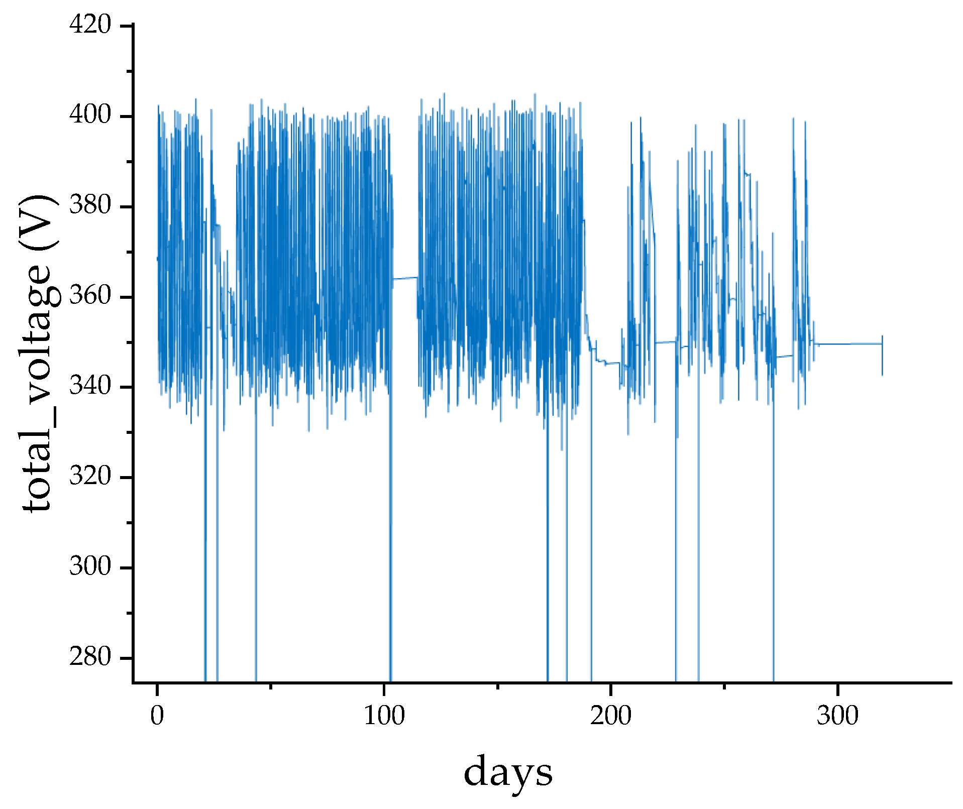
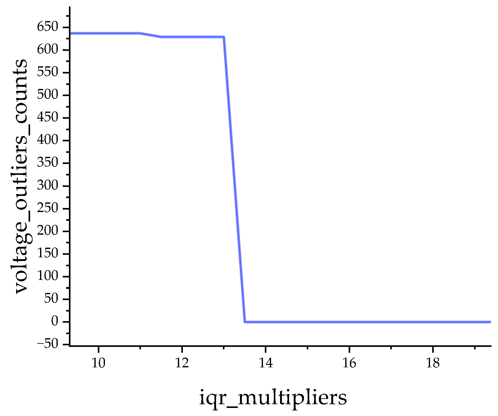
• Mild outliers: data points that moderately deviate from the central values and occur with relatively high frequency.
• Extreme outliers: isolated points that show substantial deviations from central values.

By categorizing outliers into mild and extreme, this approach ensures only extreme outliers are removed, preserving data quality.

Since the proportion of missing and outlier-removed values in the data is less than 0.1%, linear interpolation is directly used to fill in the gaps.

2.3. Trip Segmentation

The focus of this study is on trip-level energy consumption analysis. After filtering outliers and interpolating missing data, the real-time discharge cycles were segmented into individual trips. Trip segmentation was performed by matching vehicle GPS coordinates (latitude and longitude) with known station locations. A trip was identified when the following conditions were met:

• The vehicle location was closest to a station;
• Both vehicle speed and motor speed were zero, indicating a complete stop.

Using these criteria, the start and end points of each trip were determined. Figure 5 illustrates an example of daily discharge cycle segmentation into individual trips, where the vertical axis represents the EB State of Charge (SOC). Through this process, a total of 11,333 trips were identified for analysis.

3. Methodology

3.1. Driving Patterns Analysis

In this study, driving patterns were analyzed to extract representative features for model development. Acceleration is a fundamental parameter in our analysis, characterizing driving conditions. The instantaneous acceleration is calculated as follows:

$$a_{i+1}={\displaystyle \frac{v_{i+1}-v_i}{t_{i+1}-t_i}}\times {\displaystyle \frac{1000}{3600}}\left(\mathrm{m}/{\mathrm{s}}^2\right)$$

(1)

where $a_{i+1}$ represents acceleration at time step $i+1$ ($\mathrm{m}/{\mathrm{s}}^2$), $v_{i+1}$ and $v_i$ denote velocities at respective time steps ($\mathrm{k}\mathrm{m}/\mathrm{h}$), and $t_{i+1}$ and $t_i$ represent corresponding time points (s).

During actual vehicle operation, each start and stop generates a driving segment, which includes multiple kinematic states. Segments are classified using a predefined principle when the acceleration ranges between −0.15 and 0.15 m/s² [64]. Based on kinematic characteristics, driving segments are classified into four states [65], as follows:

• Idle State ($S_{\mathrm{I}}$);
  • High-voltage system active;
  • $v=0 \mathrm{k}\mathrm{m}/\mathrm{h}$.
• Constant Speed State ($S_{\mathrm{C}}$);
  • $\left|a\right|\le 0.15 \mathrm{m}/{\mathrm{s}}^2$;
  • $v>0 \mathrm{k}\mathrm{m}/\mathrm{h}$.
• Acceleration State ($S_{\mathrm{A}}$);
  • $a>0.15 \mathrm{m}/{\mathrm{s}}^2$;
  • $v>0 \mathrm{k}\mathrm{m}/\mathrm{h}$.
• Deceleration State ($S_{\mathrm{D}}$).
  • $a<-0.15 \mathrm{m}/{\mathrm{s}}^2$;
  • $v>0 \mathrm{k}\mathrm{m}/\mathrm{h}$.

Vehicle operation is a complex process, requiring the selection of an appropriate number of feature parameters to evaluate these kinematic segments. Classifying kinematic segments assists in identifying key parameters, and selecting both commonly used parameters and those potentially useful in describing driving conditions. In addition to the usual 9 feature parameters, extra parameters were incorporated for kinematic segment extraction based on studies from Shanghai [66] and Dalian [67]. Ultimately, we identified 13 characteristic parameters that capture various aspects of vehicle operation, detailed in

Table 3. 13 Driving characteristic parameters.

Characteristic	Symbol	Unit
Idle Time Ratio	$R_{\mathrm{i}\mathrm{d}}$	%
Acceleration Time Ratio	$R_{\mathrm{a}}$	%
Deceleration Time Ratio	$R_{\mathrm{d}}$	%
Constant Speed Time Ratio	$R_{\mathrm{c}}$	%
Average Speed	$V_{\mathrm{a}\mathrm{v}\mathrm{e}}$	km/h
Average Travel Speed	$V_{\mathrm{a}\mathrm{v}\mathrm{e}\_\mathrm{t}\mathrm{r}\mathrm{a}\mathrm{v}\mathrm{e}\mathrm{l}}$	km/h
Maximum Speed	$V_{\mathrm{m}\mathrm{a}\mathrm{x}}$	km/h
Speed Standard Deviation	$V_{\mathrm{s}\mathrm{t}\mathrm{d}}$	km/h
Maximum Acceleration	$a_{\mathrm{m}\mathrm{a}\mathrm{x}}$	$\mathrm{m}/{\mathrm{s}}^2$
Maximum Deceleration	$d_{\mathrm{m}\mathrm{a}\mathrm{x}}$	$\mathrm{m}/{\mathrm{s}}^2$
Average Acceleration	$a_{\mathrm{a}\mathrm{v}\mathrm{e}}$	$\mathrm{m}/{\mathrm{s}}^2$
Average Deceleration	$d_{\mathrm{a}\mathrm{v}\mathrm{e}}$	$\mathrm{m}/{\mathrm{s}}^2$
Acceleration-Deceleration Standard Deviation	$a_{\mathrm{s}\mathrm{t}\mathrm{d}}$	$\mathrm{m}/{\mathrm{s}}^2$

.

The calculation methods of the 13 features are as follows:

• Idle Time Ratio;

$$R_{\mathrm{i}\mathrm{d}}={\displaystyle \frac{T_{\mathrm{i}\mathrm{d}}}{T}}\times 100\%$$

(2)

where $T_{\mathrm{i}\mathrm{d}}$ is the total duration of the idle state (high-voltage system active; $v=0 \mathrm{k}\mathrm{m}/\mathrm{h}$), and $T$ is the total duration of the driving segment.

2.

Acceleration Time Ratio;

$$R_{\mathrm{a}}={\displaystyle \frac{T_{\mathrm{a}}}{T}}\times 100\%$$

(3)

where $T_{\mathrm{a}}$ is the total duration in the acceleration state ($a>0.15 \mathrm{m}/{\mathrm{s}}^2,v>0 \mathrm{k}\mathrm{m}/\mathrm{h}$).

3.

Deceleration Time Ratio;

$$R_{\mathrm{d}}={\displaystyle \frac{T_{\mathrm{d}}}{T}}\times 100\%$$

(4)

where $T_{\mathrm{d}}$ is the total duration in the acceleration state ($a<-0.15 \mathrm{m}/{\mathrm{s}}^2,v>0 \mathrm{k}\mathrm{m}/\mathrm{h}$).

4.

Constant Speed Time Ratio;

$$R_{\mathrm{c}}={\displaystyle \frac{T_{\mathrm{c}}}{T}}\times 100\%$$

(5)

where $T_{\mathrm{c}}$ is the total duration of the constant speed state ($\left|a\right|\le 0.15 \mathrm{m}/{\mathrm{s}}^2,v>0 \mathrm{k}\mathrm{m}/\mathrm{h}$).

5.

Average Speed;

The average speed $V_{\mathrm{a}\mathrm{v}\mathrm{e}}$ represents the mean velocity of a vehicle during its active motion periods, excluding all idle time ($T_{\mathrm{i}\mathrm{d}}$). It is calculated as follows:

$$V_{\mathrm{a}\mathrm{v}\mathrm{e}}={\displaystyle \frac{S}{T-T_{\mathrm{i}\mathrm{d}}}}$$

(6)

where $S$ is the distance traveled, calculate $S$ from the following:

$$S={\displaystyle \sum _{i=1}^k}{v}_i·t_i$$

(7)

where $v_i$ is instantaneous speed and $t_i$ is the time interval.

6.

Average Travel Speed;

The average travel speed $V_{\mathrm{a}\mathrm{v}\mathrm{e}\_\mathrm{t}\mathrm{r}\mathrm{a}\mathrm{v}\mathrm{e}\mathrm{l}}$ represents the mean velocity over the complete trip duration, including all idle periods. It is calculated as follows:

$$V_{\mathrm{a}\mathrm{v}\mathrm{e}\_\mathrm{t}\mathrm{r}\mathrm{a}\mathrm{v}\mathrm{e}\mathrm{l}}={\displaystyle \frac{S}{T}}$$

(8)

7.

Maximum Speed;

$$V_{\mathrm{m}\mathrm{a}\mathrm{x}}=\max \{V_i, i=1,2,\dots ,n\}$$

(9)

8.

Speed Standard Deviation;

$$V_{\mathrm{s}\mathrm{t}\mathrm{d}}=\sqrt{{\displaystyle \frac{1}{n-1}}{\displaystyle \sum _{i=1}^n}{\left(V_i-\overline{V_{\mathrm{a}\mathrm{v}\mathrm{e}\_\mathrm{t}\mathrm{r}\mathrm{a}\mathrm{v}\mathrm{e}\mathrm{l}}}\right)}^2}$$

(10)

9.

Acceleration-Related Parameters;

• Maximum Acceleration:

  $$a_{\mathrm{m}\mathrm{a}\mathrm{x}}=\max \{a_i,i=1,2,\dots ,n\}$$

  (11)
• Maximum Deceleration:

  $$d_{\mathrm{m}\mathrm{a}\mathrm{x}}=\min \{a_i,i=1,2,\dots ,n\}$$

  (12)
• Average Acceleration:

  $$a_{\mathrm{a}\mathrm{v}\mathrm{e}}={\displaystyle \frac{{\sum }_{a_i\ge 0.15}{a}_i,i=1,2,\dots ,n}{T_{\mathrm{a}}}}$$

  (13)
• Average Deceleration:

  $$d_{\mathrm{a}\mathrm{v}\mathrm{e}}={\displaystyle \frac{{\sum }_{a_i\le -0.15}{a}_i,i=1,2,\dots ,n}{T_{\mathrm{d}}}}$$

  (14)
• Acceleration–Deceleration Standard Deviation:

  $$a_{\mathrm{s}\mathrm{t}\mathrm{d}}=\sqrt{{\displaystyle \frac{1}{n-1}}{\displaystyle \sum _{i=1}^n}{a}_i^2}$$

  (15)

The features derived above are numerous and are largely determined through calculation, which results in relatively low computational efficiency and increased complexity in model solving. Since most extracted features are related to time, speed, and acceleration, there is correlation among different features, and redundant information may lead to an excessive number of features, increased model complexity, decreased accuracy, and weakened generalization ability. To address this issue, we utilized Principal Component Analysis (PCA) to reduce dimensionality, transforming the 13 feature parameters into a smaller set of principal components.

PCA effectively reduces feature numbers and data complexity by retaining a subset of principal components. This method transforms high-dimensional data into uncorrelated variables while preserving maximum variance. For a dataset $X\in R^{n\times \mathbb{2}}$ with $n$ observations, we use orthogonal transformation to find new coordinates $Y$ that better represent the data structure.

The transformation can be expressed in matrix form, as follows:

$$\left[\begin{array}{c}{Y}_1\\ Y_2\end{array}\right] =\left[\begin{array}{cc}\cos \left(\alpha \right)& \sin \left(\alpha \right)\\ -\sin \left(\alpha \right)& \cos \left(\alpha \right)\end{array}\right]\left[\begin{array}{c}{X}_1\\ X_2\end{array}\right]=P^{T}X$$

(16)

where $P$ is an orthogonal matrix ($P{P}^T=P^{T}P=I$), and ($Y_1$, $Y_2$) represent the principal components ordered by decreasing variance.

The implementation involves standardizing the data ($\tilde{X}=\left(X-\mu \right)/\sigma$), computing the covariance matrix ($\mathsf{\Sigma }={\displaystyle \frac{1}{n}}\widetilde{X^T}\tilde{X}$), and solving the eigenvalue equation $\mathsf{\Sigma }v=\lambda v$. The proportion of variance explained by $k$ components is given by $\eta ={\sum }_{i=1}^k{\lambda }_i/{\sum }_{i=1}^n{\lambda }_i$, enabling effective dimensionality reduction while minimizing information loss.

Through the PCA of the 13 standardized features, we identified the first four principal components as having eigenvalues greater than 1, accounting for only 71.57% of the total variance. Including the first six principal components would exceed 80% variance contribution. Thus, a compromise was made to select the inflection point in the plot, choosing the first five principal components, which collectively account for 77.85% of the total variance, as depicted in Figure 6. These five components were selected to represent the original feature set.

Table 4. Principal component loading matrix.

Characteristic	PC1	PC2	PC3	PC4	PC5
Idle Time Ratio	−0.079	−0.418	0.438	0.045	−0.361
Acceleration Time Ratio	−0.234	−0.061	0.051	0.258	0.280
Deceleration Time Ratio	0.538	−0.052	0.021	−0.547	−0.119
Constant Speed Time Ratio	0.189	−0.234	−0.096	0.113	−0.212
Average Speed	0.402	−0.424	−0.007	−0.025	0.154
Average Travel Speed	0.252	0.154	−0.407	−0.013	−0.001
Maximum Speed	−0.066	0.274	0.373	−0.555	0.206
Speed Standard Deviation	−0.164	0.213	−0.033	0.008	0.156
Maximum Acceleration	−0.212	0.093	0.349	−0.206	0.012
Maximum Deceleration	−0.125	0.373	−0.168	−0.052	−0.758
Average Acceleration	−0.022	0.085	0.061	−0.117	0.036
Average Deceleration	−0.103	−0.254	0.305	0.048	−0.257
Acceleration-Deceleration Standard Deviation	0.535	0.470	0.494	0.500	0.000

presents the Principal Component Loading Matrix, a key result of PCA, where each principal component is a linear combination of the original variables. The loading coefficients indicate the degree of contribution of each variable to the principal component. A higher loading coefficient signifies a stronger correlation between the feature value and the principal component, and vice versa.

When identifying principal components to retain, it is also essential to examine the relationship between the principal components and various feature parameters. Ensuring a strong correlation between each principal component and a specific feature parameter helps maintain a match between the selected principal components and actual data, thereby enhancing model accuracy and reliability:

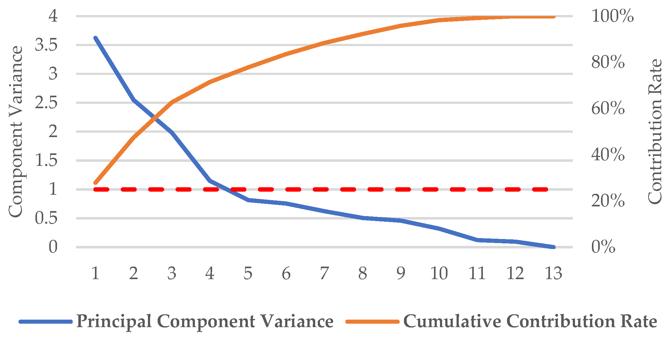
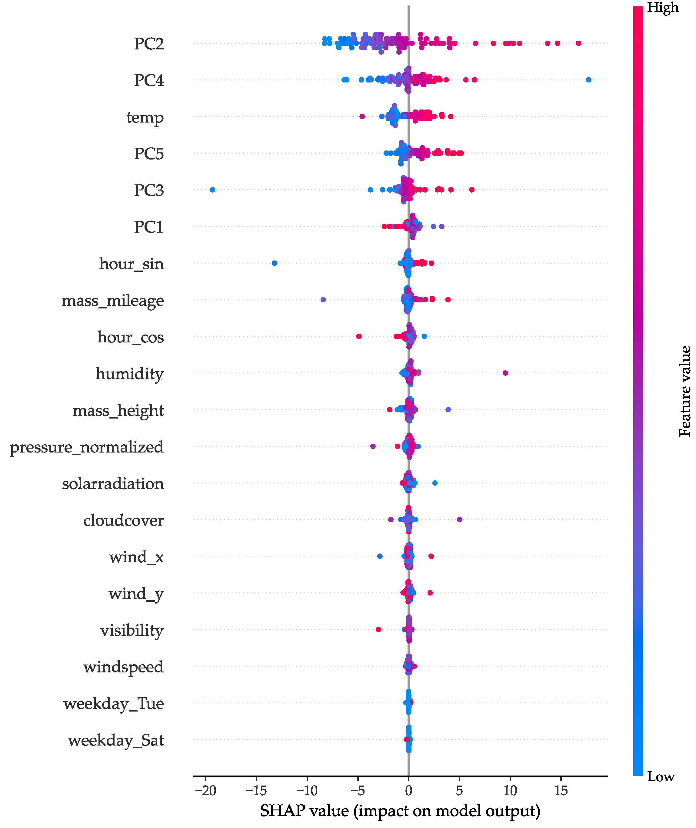
• First Principal Component (PC1): primarily describes the balance between acceleration and deceleration, with significant contributions from the Deceleration Time Ratio and Acceleration–Deceleration Standard Deviation;
• Second Principal Component (PC2): mainly characterizes variations in speed-related features, particularly the Idle Time Ratio and Average Speed;
• Third Principal Component (PC3): focuses on speed metrics and their deviations, as indicated by contributions from the Average Travel Speed and Maximum Speed;
• Fourth Principal Component (PC4): reflects the interplay of speed and acceleration, especially through contributions from Average Deceleration and Maximum Speed;
• Fifth Principal Component (PC5): primarily associated with the variability in deceleration, dominated by the Maximum Deceleration.

3.2. Energy Consumption Evaluation

3.2.1. Battery Output Power

The energy source of EBs is the output energy from their batteries, which is determined by the battery’s output power and serves as the foundation for further calculations. The total energy consumption can be expressed as follows:

$$E=\left({\displaystyle \sum _{k=1}^n}{U}_k·I_k·\mathsf{\Delta }{t}_k=\underset{Battery\hspace{0.25em}Energy\hspace{0.25em}\left(E_{\mathrm{b}}\right)}{\underbrace{\sum _{I_k>0}{U}_k·I_k·\mathsf{\Delta }{t}_k}}+\underset{Regenerative\hspace{0.25em}Energy\hspace{0.25em}\left(E_{\mathrm{r}}\right)}{\underbrace{\sum _{I_k<0}{U}_k·I_k·\mathsf{\Delta }{t}_k}}\right)\times {\displaystyle \frac{1}{\mathrm{3,600,000}}}$$

(17)

where

• $E$ represents the net energy consumption [kWh];
• $U_k$ is the battery voltage at time step $k$ [V];
• $I_k$ represents the battery current at time step $k$ [A], positive for discharge and negative for charging;
• $\mathsf{\Delta }{t}_k$ is the sampling time interval [s];
• $n$ is the total number of sampling points.

Brake energy regeneration, as shown in Figure 7, is a process where the electric motor captures excess energy during coasting or braking, converts it into electrical power, and recharges the battery to support subsequent acceleration. This technology is a key feature of modern electric and hybrid vehicles, and thus, net energy consumption must be taken into account during energy calculations.

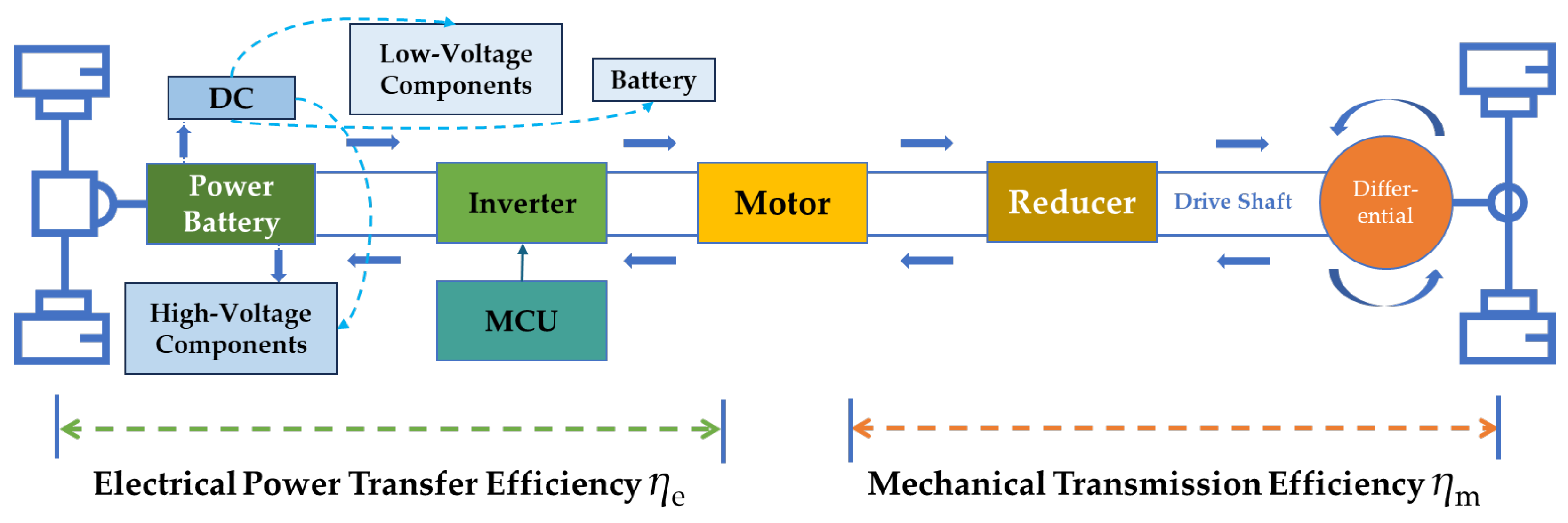
3.2.2. Traction Modeling

The energy output from the battery involves multiple efficiency factors, including battery internal efficiency, power transfer efficiency, and mechanical transmission efficiency [68]. While the battery’s internal efficiency is inherently reflected in the battery management system (BMS) measurements [69], the actual energy consumed during each trip of EBs is further affected by downstream conversion losses. The energy output from the battery is not entirely equivalent to the actual energy consumed during each trip of EBs. The electric motor converts electrical energy into mechanical energy, driving the vehicle via the transmission system. However, over time, factors such as internal motor wear, heat accumulation, and magnetic losses can lead to performance degradation in the motor [70]. Compared to internal combustion engine vehicles, electric vehicles have simpler transmission systems, primarily consisting of components like reducers and drivetrains, which ensure normal vehicle operation and interrupt power transmission when necessary. Over long-term use, the wear of the transmission components can cause a gradual decrease in mechanical transmission efficiency [71], potentially leading to significant errors in energy consumption predictions. The main components of the vehicle include the battery, DC/AC inverter, electric motor, and transmission system, each with its own efficiency [72]. To dynamically assess the post-battery conversion efficiencies, a traction model is constructed based on the energy transfer chain, divided into the electrical power transfer stage with MCU (Motor Control Unit) and mechanical transmission, as shown in Figure 8. The model calculates two efficiencies: the electrical power transfer efficiency (${\eta }_{\mathrm{e}}$) of the traction motor and the mechanical transmission efficiency (${\eta }_{\mathrm{m}}$) of the drivetrain. These efficiencies are used to determine the energy actually utilized in vehicle operation.

1.

Electrical Power Transfer Efficiency (${\eta }_{\mathrm{e}}$);

The energy conversion process from electrical to mechanical power in the traction motor involves various losses. The average monthly electrical power transfer efficiency is calculated based on the motor’s input and output power over time, as follows:

• Traction Motor Output Power [73] ($P_{\mathrm{m}\mathrm{o}\mathrm{t}\mathrm{o}\mathrm{r}}$):

$$P_{\mathrm{m}\mathrm{o}\mathrm{t}\mathrm{o}\mathrm{r}}={\displaystyle \frac{n·T}{9.55}}$$

(18)

where $n$ represents motor rotational speed [rpm] and $T$ denotes motor torque [Nm].

• Electrical Input Power ($P_{\mathrm{D}\mathrm{C}}$):

$$P_{\mathrm{D}\mathrm{C}}=U·I$$

(19)

where $U$ represents the DC bus voltage [V] and $I$ is the DC bus current [A].

Hence, the electrical power transfer efficiency is as follows:

$${\eta }_{\mathrm{e}}={\displaystyle \frac{P_{\mathrm{m}\mathrm{o}\mathrm{t}\mathrm{o}\mathrm{r}}}{P_{\mathrm{D}\mathrm{C}}}}$$

(20)

2.

Mechanical Transmission Efficiency (${\eta }_{\mathrm{m}}$);

In constant-speed operation, the mechanical power output equals the driving resistance power. Therefore, only constant-speed states are considered when calculating mechanical transmission efficiency. Driving resistance power includes acceleration resistance, slope resistance, rolling resistance, and air resistance. However, in steady states, acceleration resistance is zero, and changes in road slopes on urban routes are typically minor and have a negligible impact on energy consumption [74]. Therefore, driving resistance is calculated only considering rolling resistance and air resistance in constant-speed conditions.

●

Rolling Resistance Force [75,76] ($F_{\mathrm{r}\mathrm{o}\mathrm{l}\mathrm{l}\mathrm{i}\mathrm{n}\mathrm{g}}$):

$$F_{\mathrm{r}\mathrm{o}\mathrm{l}\mathrm{l}\mathrm{i}\mathrm{n}\mathrm{g}}=f·M·g$$

(21)

where

•

$f=0.02$ (rolling resistance coefficient);

•

$M=\mathrm{11,800} \mathrm{k}\mathrm{g}$ (vehicle mass);

•

$g=9.81 \mathrm{m}/{\mathrm{s}}^2$ (gravitational acceleration);

●

Aerodynamic Drag Force [77] ($F_{\mathrm{a}\mathrm{i}\mathrm{r}}$):

$$F_{\mathrm{a}\mathrm{i}\mathrm{r}}={\displaystyle \frac{C_{\mathrm{D}}·A·u_{\mathrm{a}}^2}{21.15}}$$

(22)

where

•

$C_{\mathrm{D}}=0.8$ (aerodynamic drag coefficient for buses);

•

$A=7.1655{ \mathrm{m}}^2$(frontal area);

•

$u_{\mathrm{a}}=$ vehicle velocity [$\mathrm{m}/{\mathrm{s}}^2$].

Consequently, the driving resistance power is as follows:

$$P_{\mathrm{r}\mathrm{e}\mathrm{s}\mathrm{i}\mathrm{s}\mathrm{t}\mathrm{a}\mathrm{n}\mathrm{c}\mathrm{e}}=\left(F_{\mathrm{r}\mathrm{o}\mathrm{l}\mathrm{l}\mathrm{i}\mathrm{n}\mathrm{g}}+F_{\mathrm{a}\mathrm{i}\mathrm{r}}\right)·u_{\mathrm{a}}=713.22·u_{\mathrm{a}}+0.0753·u_{\mathrm{a}}^3$$

(23)

The mechanical transmission efficiency quantifies power losses in the drivetrain components:

●

Mechanical Input Power at Constant Speed ($P_{\mathrm{m}\mathrm{o}\mathrm{t}\mathrm{o}\mathrm{r}-\mathrm{c}\mathrm{o}\mathrm{n}\mathrm{s}\mathrm{t}\mathrm{a}\mathrm{n}\mathrm{t}}$):

$$P_{\mathrm{m}\mathrm{o}\mathrm{t}\mathrm{o}\mathrm{r}-\mathrm{c}\mathrm{o}\mathrm{n}\mathrm{s}\mathrm{t}\mathrm{a}\mathrm{n}\mathrm{t}}={\displaystyle \frac{n·T}{9.55}}$$

(24)

Thus, the mechanical transmission efficiency is as follows:

$${\eta }_{\mathrm{m}}={\displaystyle \frac{P_{\mathrm{r}\mathrm{e}\mathrm{s}\mathrm{i}\mathrm{s}\mathrm{t}\mathrm{a}\mathrm{n}\mathrm{c}\mathrm{e}}}{P_{\mathrm{m}\mathrm{o}\mathrm{t}\mathrm{o}\mathrm{r}-\mathrm{c}\mathrm{o}\mathrm{n}\mathrm{s}\mathrm{t}\mathrm{a}\mathrm{n}\mathrm{t}}}}$$

(25)

3.

System-Level Energy Transfer Efficiency (${\eta }_{\mathrm{s}}$);

The overall system efficiency is the product of both component efficiencies:

$${\eta }_{\mathrm{s}}={\eta }_{\mathrm{e}}\times {\eta }_{\mathrm{m}}=\left({\displaystyle \frac{P_{\mathrm{motor}}}{P_{\mathrm{DC}}}}\right)\times \left({\displaystyle \frac{P_{\mathrm{resistance}}}{P_{\mathrm{m}\mathrm{o}\mathrm{t}\mathrm{o}\mathrm{r}-\mathrm{c}\mathrm{o}\mathrm{n}\mathrm{s}\mathrm{t}\mathrm{a}\mathrm{n}\mathrm{t}}}}\right)$$

(26)

This approach provides a more accurate measure of energy consumption, helping improve the model’s predictive accuracy.

3.3. LightGBM Algorithm Description

LightGBM is a boosting ensemble model developed by Microsoft [78], known for its optimized and efficient implementation of Gradient Boosting Decision Trees (GBDTs) [79]. While similar to eXtreme Gradient Boosting (XGBoost), LightGBM often shows superior performance in various circumstances.

Handling large datasets is essential for many applications. Unlike deep learning algorithms, which use mini-batches to train networks and circumvent memory constraints, traditional machine learning algorithms like GBDT require multiple iterations over the entire training set. This need to load the entire dataset into memory can restrict dataset size, and frequent reading and writing would be time-prohibitive [80].

Standard GBDT algorithms face challenges when dealing with industrial-scale data. To address these issues, LightGBM was designed to efficiently train GBDT models on large datasets [81]. It employs a histogram-based algorithm [82], as shown in Figure 9 [83,84], that reduces memory usage and simplifies data segmentation by the following:

• Discretizing continuous floating-point features into discrete bins and creating histograms of a fixed width.
• Iterating through the training data to accumulate statistics for each discrete bin in the histogram.
• Determining the optimal split point by iterating over the histogram bins during feature selection.

This histogram method reduces memory consumption by storing only discretized feature values instead of additional storage for pre-sorted data. A few bits typically suffice to represent these values.

LightGBM also uses a leaf-wise growth strategy [85], depicted in Figure 10 [86,87], unlike the level-wise strategy used by algorithms like CatBoost [88] and XGBoost. This strategy allows for more precise data fitting, enhancing model performance. At each step, LightGBM identifies and splits the leaf with the highest split gain, usually the one with the largest data volume. Compared to level-wise methods, leaf-wise growth reduces errors for the same number of splits, leading to better accuracy. However, it can produce deep trees and risk overfitting, which LightGBM mitigates by setting a maximum depth limit, balancing efficiency and preventing overfitting.

Mathematically, LightGBM’s boosting process involves minimizing a loss function $L$, often represented as the following:

$$L\left(y,F\left(x\right)\right)={\displaystyle \sum _{i=1}^n}l\left(y_i,F\left(x_i\right)\right)$$

(27)

where $y$ denotes the target value, $F\left(x\right)$ is the predicted output, $l$ is the loss function, and the sum runs over all $n$ observations. The model aims to find the function $F$ that minimizes $L$.

LightGBM introduces Gradient-based One-Side Sampling (GOSS), which retains instances with large gradients while randomly sampling those with smaller gradients [89]. This approach focuses on instances where the model’s prediction is less accurate, emphasizing difficult-to-predict examples without compromising accuracy. The large gradient instances are critical for precise model updates, while a subset of small gradient instances ensures diversity without significant computational cost. LightGBM also incorporates Exclusive Feature Bundling (EFB), which reduces dimensionality by combining mutually exclusive features [90]. When features rarely take non-zero values simultaneously, they can be bundled into a single feature without losing information, further improving computational efficiency and reducing memory usage.

LightGBM is renowned for its fast training speeds and lower memory requirements, often outperforming competitors like CatBoost and GBM. Particularly on large datasets, it significantly decreases runtime through its leaf-wise strategy and optimizes computational resource allocation. LightGBM’s capability to handle high-dimensional, large-scale datasets makes it ideal for complex and scalable applications requiring high accuracy [91]. It consistently achieves high predictive performance across various tasks, frequently surpassing other algorithms in both classification and regression, especially with high-dimensional data.

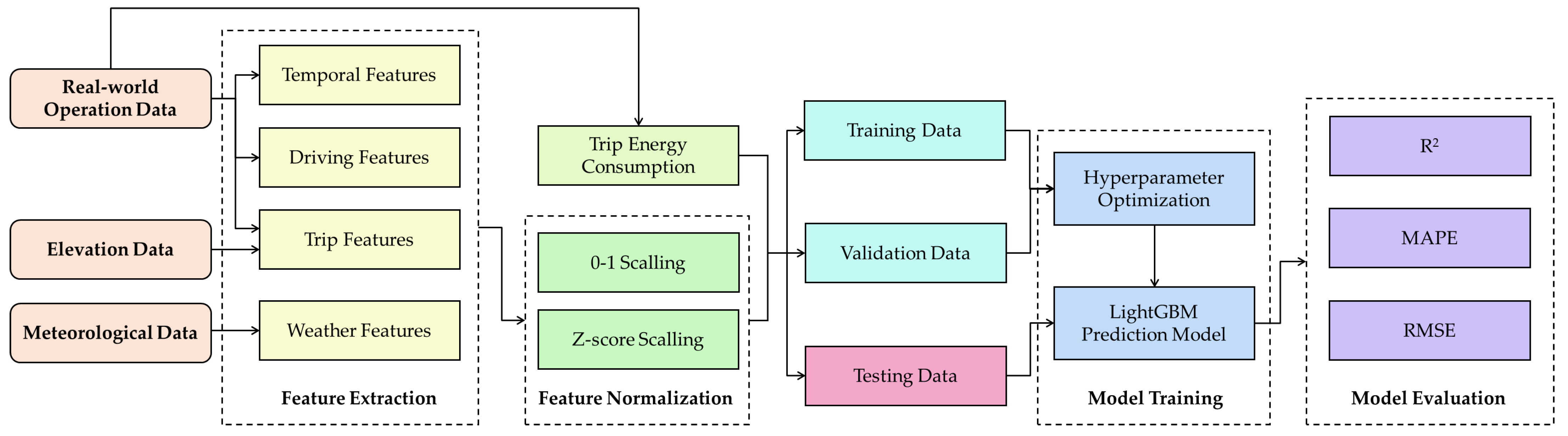
3.4. Trip-Level Energy Consumption Prediction Model Construction

The final trip-level energy consumption prediction model, illustrated in Figure 11, is constructed through four steps: feature extraction, feature normalization, model training, and model evaluation.

3.4.1. Feature Extraction

• Temporal Features;

Time-related features are crucial for understanding the operational characteristics of bus schedules, as they exhibit both time and date periodicity. In contrast to previous methods that segmented time into periods like rush hours and used one-hot encoding, leading to high-dimensional sparse matrices, we transform continuous hour values into cyclical features using sine and cosine functions, mapping each hour onto a unit circle. This method captures the periodic nature of time (24 h cycles), avoiding discontinuities between adjacent times, such as 23:59 and 00:00. The transformations are calculated as follows:

$$\mathrm{hour}\_\sin =\sin \left({\displaystyle \frac{2\mathsf{\pi }·\mathrm{hour}}{24}}\right),\mathrm{hour}\_\cos =\cos \left({\displaystyle \frac{2\pi ·\mathrm{hour}}{24}}\right)$$

(28)

For example, transforming 3:00 yields sine and cosine values both approximately 0.707, whereas 15:00 results in about −0.707 for both. This mapping ensures smooth transitions between neighboring hours (e.g., 11:00 and 12:00 are adjacent on the circle) and aligns antipodal hours symmetrically (e.g., 6:00 and 18:00), enhancing the model’s capacity to understand temporal relationships without misinterpreting cyclical boundaries.

Furthermore, we encode weekdays using one-hot encoding, translating categorical data from Monday (0) to Sunday (6) into a binary format suitable for machine learning models. These encoding strategies collectively enhance the model’s ability to leverage time-related information accurately and efficiently.

2.

Driving Features;

The features are derived using the five principal components, PC1 through PC5, for each trip as described earlier.

3.

Trip Features;

When analyzing trip features, it is essential to consider the impact of passenger load, as this factor is inherently related to the distance between stops and the elevation changes along the route. However, the original data do not include passenger load information, and it is challenging to obtain in reality. To address this, we can construct energy consumption prediction features for EBs by inferring dynamic mass through the motor torque ($T$) and acceleration ($a$). This approach indirectly reflects the impact of passenger load. By rearranging the vehicle dynamics formula, we can estimate the total mass as follows:

$$M^{\prime }={\displaystyle \frac{T}{a·r}}$$

(29)

where

• $M\prime$ is the dynamically estimated total mass (including passenger load);
• $T$ represents motor torque;
• $a$ is vehicle acceleration;
• $r$ is the wheel radius.

Given that the unloaded mass is $M_0$, the change in mass due to passenger load ($\mathsf{\Delta }M$) can be calculated by the following:

$$\mathsf{\Delta }M=M^{\prime }-M_0$$

(30)

The value of $\mathsf{\Delta }M$ can indirectly represent the passenger load, and we then integrate passenger load, stop distance, and elevation differences into input features through product summation:

• Sum of product of load and stop distances.

This feature reflects the combined effect of mass and distance, inspired by mechanical work in physics. When driving on flat terrain, the mechanical work conducted by the vehicle to overcome rolling friction and air resistance can be approximated as follows:

$$W_{\mathrm{friction}}=F_{\mathrm{friction}}·d=\left({\mu }_{\mathrm{rolling}}·M·g\right)·d$$

(31)

Here, $M$ is the total mass (including passenger load), $d$ is the distance between stops, $g$ is gravitational acceleration, and ${\mu }_{\mathrm{rolling}}$ is the rolling friction coefficient. Energy consumption is approximately positively correlated with $M·d$. Higher passenger load ($M$) and longer travel distances ($d$) result in greater energy loss due to rolling friction. Summing up $M·d$ across segments provides a comprehensive reflection of the load’s contribution to total energy consumption.

• Sum of product of load and elevation difference

This feature captures the “mass-elevation difference interaction”, emphasizing the physical essence of “overcoming potential energy change”. Elevation data for stops can be obtained via Google Earth. When a vehicle ascends an elevation $\mathsf{\Delta }h$, the potential energy changes as follows:

$$W_{\mathrm{potential}}=M·g·\mathsf{\Delta }h$$

(32)

Thus, energy consumption is directly related to $M·\mathsf{\Delta }h$. The impact of elevation difference on energy consumption is highly dependent on the load; ascending or descending energy consumption varies greatly when the vehicle is unloaded versus fully loaded. By accumulating $M·\mathsf{\Delta }h$ across segments, we can roughly estimate the energy consumption from total potential energy changes.

The features $M·d$ and $M·\mathsf{\Delta }h$ capture two factors related to passenger load, aligning well with the energy consumption model in physics:

• Assumption of linear additivity: energy consumption across segments is roughly additive, adhering to the common practice of piecewise linearization in engineering.
• Data availability: with available stop distances, elevation differences, and dynamic mass estimates ($\mathsf{\Delta }M=M^{\prime }-M_0$), the results can be directly calculated, making practical implementation feasible.
• Feature interpretability: The design of these features intuitively reflects the physical sources of energy consumption, aiding in identifying key influencing factors during model analysis. By summing the products of mass-distance and mass-elevation differences, we effectively capture the core physical mechanisms of vehicle energy consumption.
• Strong model interpretability: Feature design adheres to the law of conservation of energy, facilitating causal analysis in real-world scenarios.

Combining these features with other operating parameters can further enhance the accuracy of the energy consumption prediction model.

4.

Weather Features;

The weather data are gathered hourly from meteorological stations situated near the bus route, providing precise and real-time environmental observations. The raw dataset includes the following parameters, as shown in

Table 5. Overview of weather data variables.

Parameter	Description	Unit
temp	Ambient temperature	°C
humidity	Relative humidity	%
precip	Precipitation (rain/snow)	mm
windspeed	Wind speed	m/s
winddir	Wind direction (raw 0–360° azimuth)	degrees
cloudcover	Cloud coverage	%
visibility	Horizontal visibility	km
solarradiation	Incident solar radiation	W/m2
solarenergy	Cumulative solar energy	MJ/m2
uvindex	Ultraviolet radiation intensity	Index (0–11+)
sealevelpressure	Sea-level atmospheric pressure	hPa

.

Since the wind direction (winddir, 0–360°) is a circular variable, it can be challenging for predictive models to interpret. To resolve this, wind direction is broken down into east–west (wind_x) and north–south (wind_y) vector components using trigonometric functions:

$$\mathrm{wind}\_\mathrm{x}=\mathrm{windspeed}\times \sin \left({\displaystyle \frac{\pi \times \mathrm{winddir}}{180}}\right)$$

(33)

$$\mathrm{wind}\_\mathrm{y}=\mathrm{windspeed}\times \cos \left({\displaystyle \frac{\pi \times \mathrm{winddir}}{180}}\right)$$

(34)

This transformation converts directional information into two linearly interpretable features, where:

• A positive wind_x value indicates an eastward wind, while a negative value indicates a westward wind.
• A positive wind_y value indicates a northward wind, while a negative value indicates a southward wind.

To correct for baseline biases caused by regional elevation differences, raw atmospheric pressure values (sealevelpressure) are standardized. The normalization formula is the following:

$$\mathrm{pressure}\_\mathrm{normalized}={\displaystyle \frac{\mathrm{sealevelpressure}-1013.25}{10}}$$

(35)

Here, 1013.25 hPa represents the global average sea-level pressure. Dividing by 10 scales the normalized values into a practical range for machine learning applications.

3.4.2. Feature Normalization

The normalization of extracted features is essential to prevent model parameters from being disproportionately influenced by variables with varying scales. This process aligns data distributions across dimensions, thereby providing balanced model inputs and significantly enhancing optimization efficiency and predictive accuracy.

We employ a two-step approach: linear normalization for bounded feature alignment, followed by z-score standardization for features requiring rescaling to zero-mean and unit variance.

• Step 1: Linear Normalization

Features are scaled to the [0, 1] interval using Equation (36), which mitigates the impact of outliers in bounded features:

$$x_{\mathrm{n}\mathrm{o}\mathrm{r}\mathrm{m}}={\displaystyle \frac{x-x_{\mathrm{m}\mathrm{i}\mathrm{n}}}{x_{\mathrm{m}\mathrm{a}\mathrm{x}}-x_{\mathrm{m}\mathrm{i}\mathrm{n}}}}$$

(36)

where $x$ is the original feature value, $x_{\mathrm{m}\mathrm{i}\mathrm{n}}$ and $x_{\mathrm{m}\mathrm{a}\mathrm{x}}$ represent the minimum and maximum values within the feature set, and $x_{\mathrm{n}\mathrm{o}\mathrm{r}\mathrm{m}}$ is the normalized output.

• Step 2: Z-Score Standardization

For features with unbounded ranges or Gaussian-like distributions, standardization via Equation (37) ensures a mean of 0 and a standard deviation of 1:

$$x_{\mathrm{standard}}={\displaystyle \frac{x-\mu }{\sigma }}$$

(37)

where $\mu$ and $\sigma$ denote the feature’s mean and standard deviation, respectively.

This dual strategy ensures both dimensionally uniform inputs and stable gradient updates during training, accelerating model convergence.

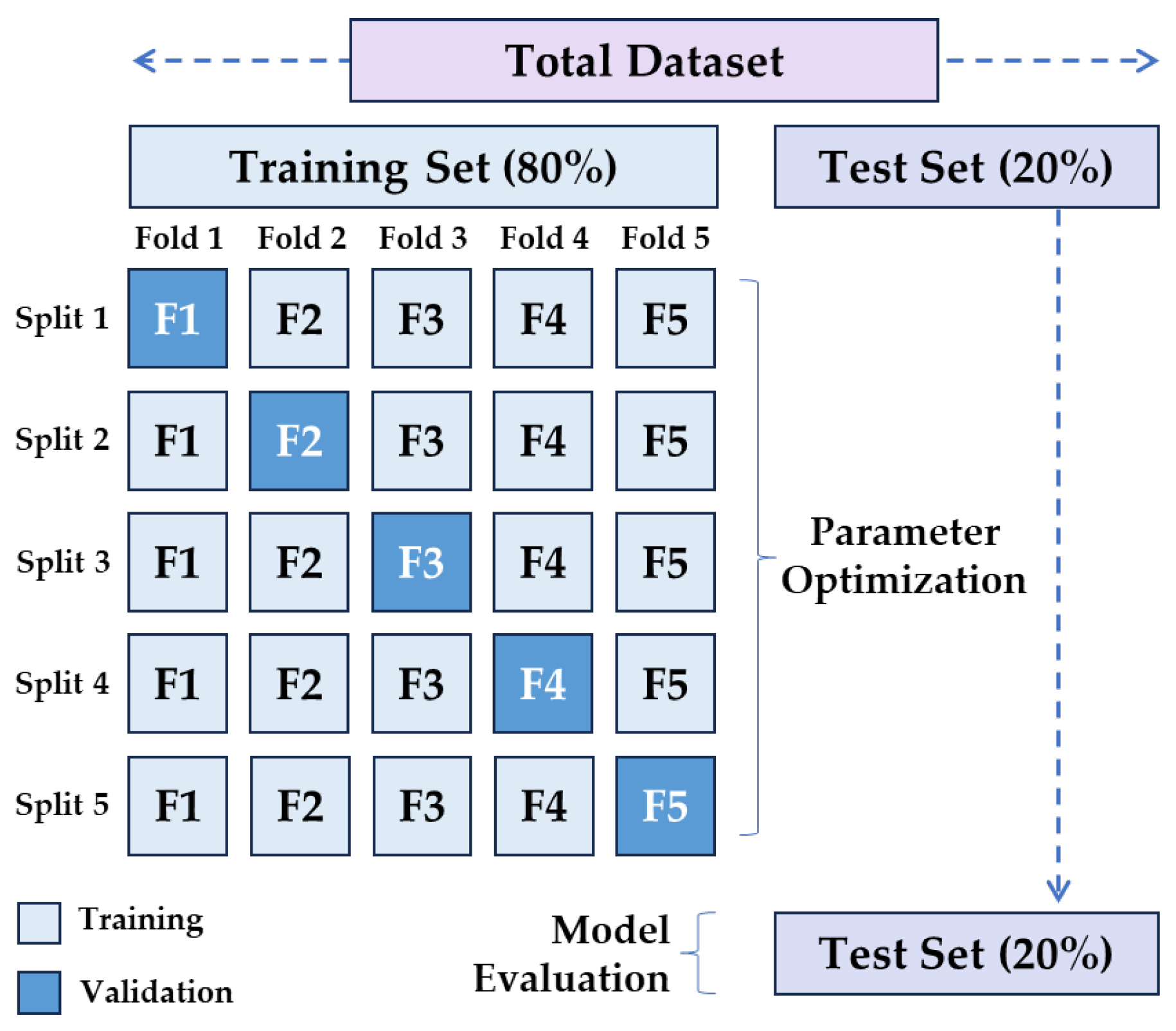
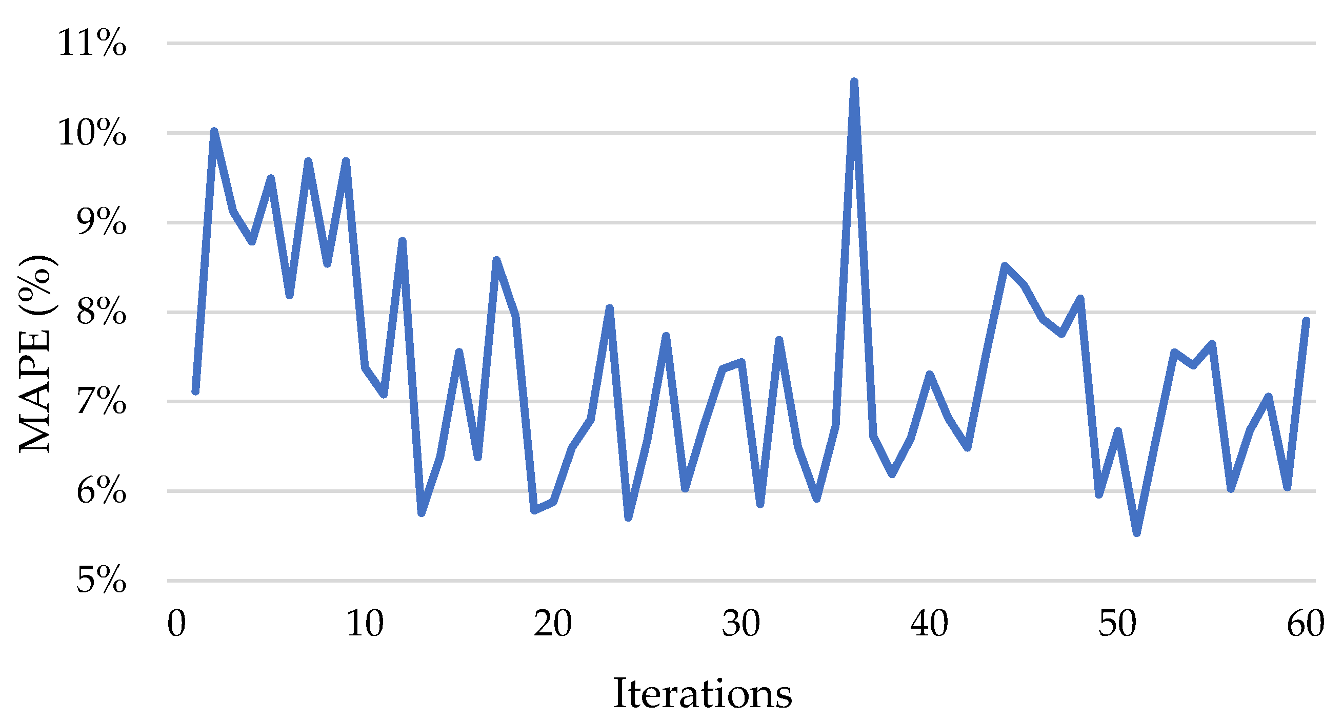
3.4.3. Model Training

The dataset was randomly partitioned, with 80% randomly selected for the training set and the remaining 20% allocated to the test set. As shown in Figure 12, a 5-fold cross-validation approach was applied to the training set, where each fold used 80% of the data for training and 20% for validation.

The primary training objective was to minimize the discrepancy between the predicted and actual energy consumption per trip. To achieve this, Bayesian Optimization (BO)—a global probabilistic approach [92]—was implemented for hyperparameter tuning. BO outperforms grid and random search in scenarios with costly objective evaluations by iteratively updating a surrogate model (Gaussian Process [93]) and effectively balancing exploration–exploitation through acquisition functions.

The optimization problem is defined as follows:

$$x^{*}=\mathrm{a}\mathrm{r}\mathrm{g}\underset{x\in \mathcal{X}}{\min } f\left(x\right) \mathrm{s}.\mathrm{t}.\left\{\begin{array}{c}5\le \text{max\_depth}\le 25,\\ 100\le \text{n\_estimators}\le 800,\\ 0.01\le \text{learning\_rate}\le 0.3,\\ 0.6\le \text{subsample}\le 1.0,\\ 0\le \text{reg\_alpha}\le 1\end{array}\right.$$

(38)

where $f\left(x\right)$ represents the objective function, and the constraints define the feasible hyperparameter space [94] for the LightGBM model based on common practices [95] in gradient boosting algorithms and preliminary experiments to achieve a balance between model performance and computational efficiency.

To assess the model’s performance during hyperparameter optimization, we used the Mean Absolute Percentage Error (MAPE). The MAPE quantifies accuracy in percentage terms, highlighting the average deviation of the prediction from the actual values.

$$MAPE={\displaystyle \frac{100\%}{n}}{\displaystyle \sum _{i=1}^n}\left|{\displaystyle \frac{y_i-\widehat{y_i}}{y_i}}\right|$$

(39)

Here, $y_i$ represents the actual values and $\widehat{y_i}$ denotes the predicted values. A lower MAPE value indicates a more precise forecast.

As illustrated in Figure 13, the BO algorithm achieves and maintains strong performance throughout the optimization process, with MAPE values generally staying between 5.5% and 8.5%, and reaching its best performance of 5.5% at iteration 51 on the training set. As shown in

Table 6. Performance comparison after optimization techniques.

Method	Execution Time (s)	Test Set MAPE (%)
Default Params	N/A *	9.37
Grid Search	29,376.28	4.72
BO Search	708.10	3.92

* Default parameters require no hyperparameter search process.

, BO reduced the test set MAPE by 5.45 percentage points (58.2% relative reduction) compared to default hyperparameters, achieving superior performance with a final MAPE of 3.92%. This efficiency is particularly notable given that BO required 98.7% fewer evaluations than a grid search (60 iterations vs. 4752 parameter combinations), corresponding to a 97.6% reduction in execution time (708.10 s vs. 29,376.28 s).

The optimized hyperparameters obtained through BO are detailed in

Table 7. Optimized hyperparameters via BO.

Parameter	Value
learning_rate	0.298
max_depth	13
n_estimators	633
reg_alpha	0.167
subsample	0.824

.

3.4.4. Model Evaluation

To evaluate model performance after hyperparameter optimization, we use R-squared ($R^2$) and Root Mean Square Error (RMSE) metrics, in addition to MAPE. These assessments are conducted on the test dataset to confirm the model’s generalizability and effectiveness.

The $R^2$ metric is calculated as follows:

$$R^2=1-{\displaystyle \frac{{\sum }_{i=1}^n{\left(y_i-\widehat{y_i}\right)}^2}{{\sum }_{i=1}^n{\left(y_i-\overline{y}\right)}^2}}$$

(40)

where $y_i$ represents the actual energy consumption values, $\widehat{y_i}$ denotes the predicted values, and $\overline{y}$ is the mean of the actual values. $R^2$ quantifies the proportion of variance explained by the model, indicating how well the model fits the data.

In addition, we calculate the Root Mean Square Error (RMSE) as follows:

$$RMSE=\sqrt{{\displaystyle \frac{1}{n}}{\displaystyle \sum _{i=1}^n}{\left(y_i-\widehat{y_i}\right)}^2}$$

(41)

RMSE provides an absolute measure of error in the same units as the target variable (kWh). By analyzing these metrics, we obtain a comprehensive understanding of the model’s predictive performance on the test set.

4. Results and Discussion

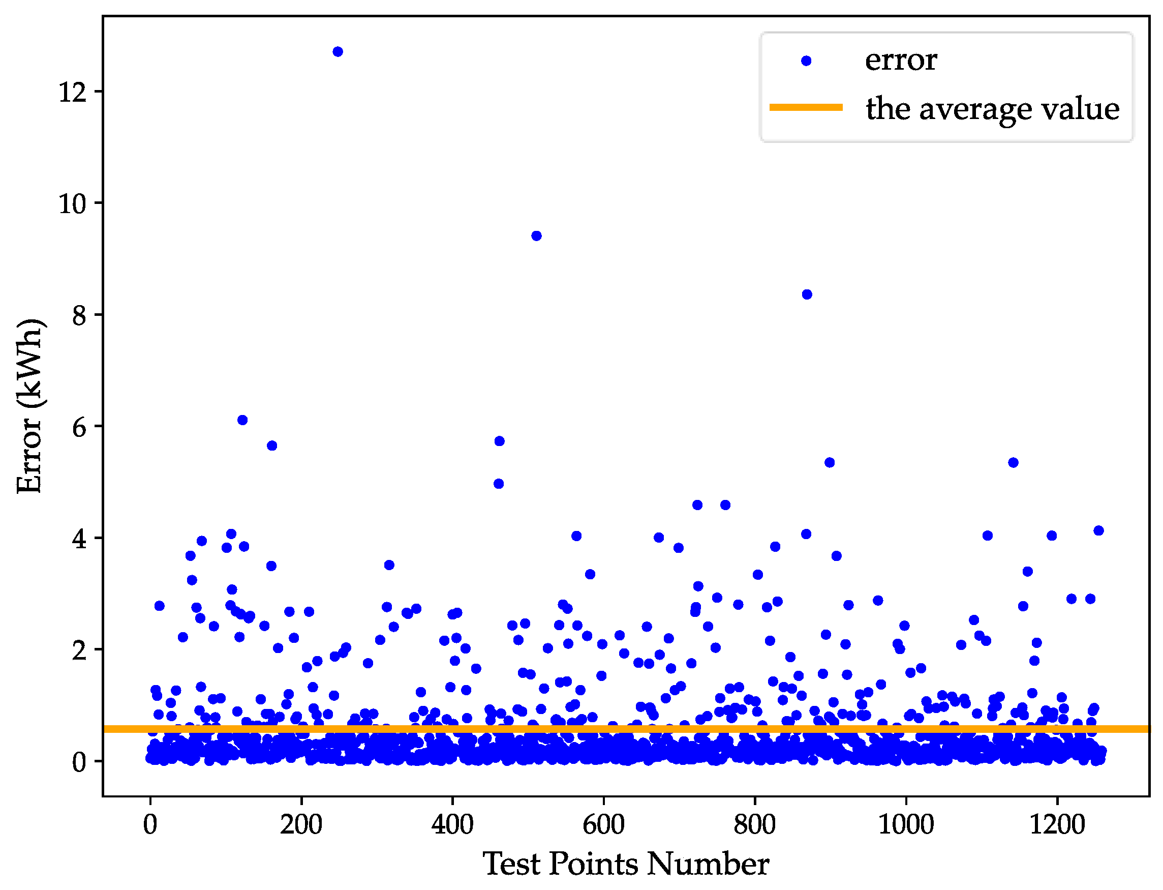
4.1. Model Validation

The proposed trip-level energy consumption prediction model achieves accurate predictions on the test set, with an average absolute error of 0.569 kWh (approximately 2.99% relative error), as shown in Figure 14. Regarding the average speed, the average total energy consumption is 19.03 kWh.

Model evaluation on the test dataset revealed exceptional performance, with an R² score exceeding 0.995, a MAPE of 3.92%, and an RMSE of 1.398 kWh, indicating strong alignment between predictions and actual values. The proposed method’s suitability for real-time trip-level energy prediction stems from the following two advantages:

• Data Accessibility: Input features (datetime, weather, trip dynamics, and driving patterns) can be directly obtained or calculated from real-time operation data or public APIs.
• Computational Efficiency: Model requires only 1.0337 s and 177.91 MB of memory on personal computer, meeting real-time operational requirements.

The model facilitates seamless integration into onboard systems, enhancing real-time trip-level energy management capabilities.

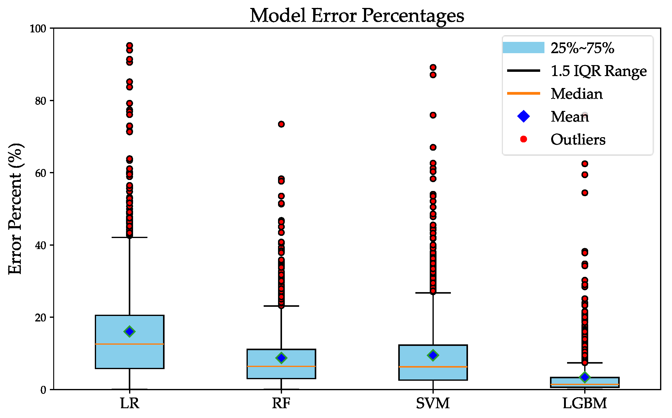
4.2. Different Algorithms’ Comparation

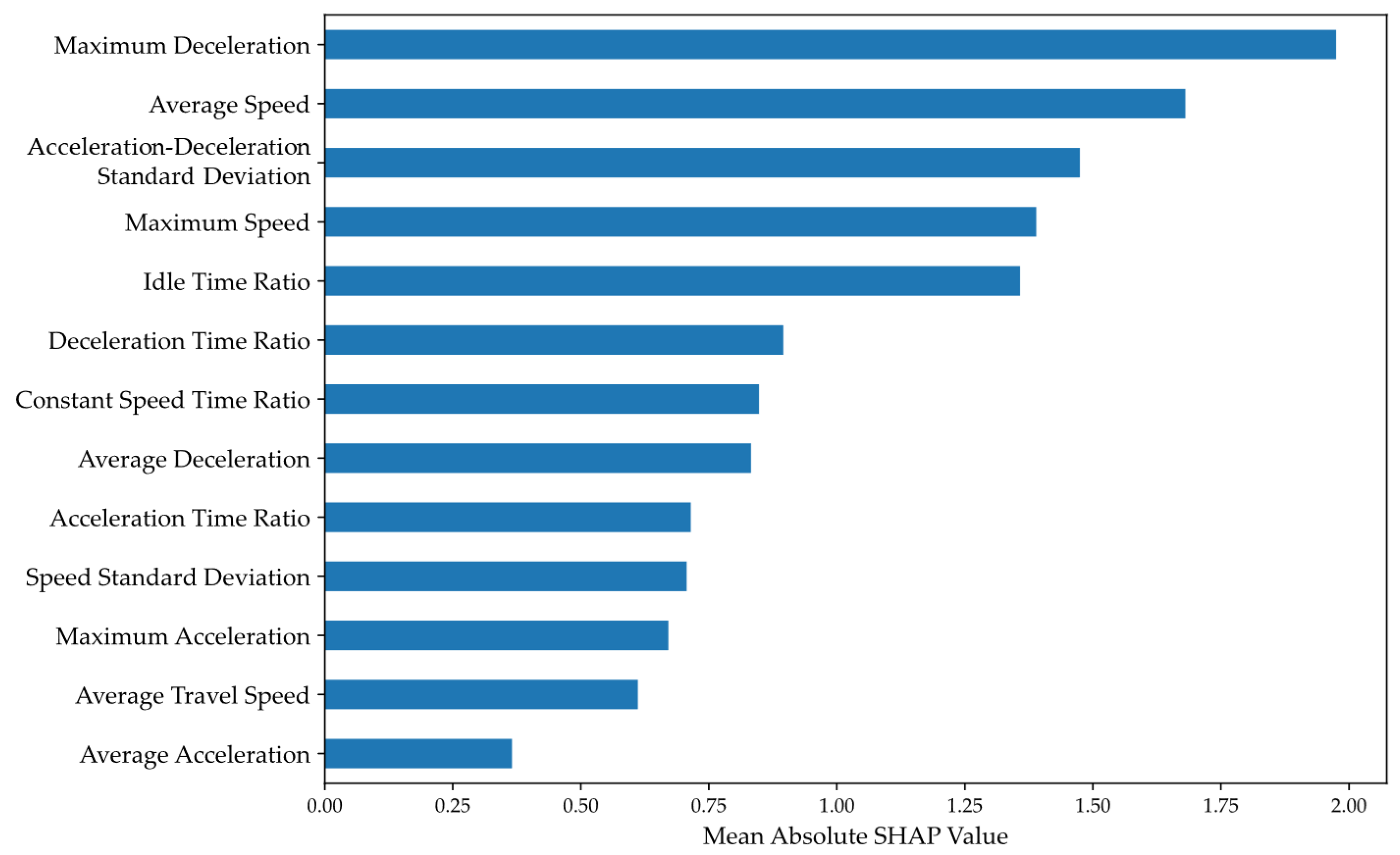
To verify the effectiveness of our approach, we compare LightGBM with linear regression (LR), random forest (RF), and support vector machine (SVM)-based algorithms. Figure 15 presents a box plot of relative prediction errors, providing a clear visual comparison of these methods. The results clearly show that LightGBM outperforms the other algorithms. It has both the smallest interquartile range (between 25% and 75%) and the lowest median error, indicating that its predictions are more consistent and accurate. These findings demonstrate that LightGBM is more reliable than traditional methods like LR, RF, and SVM for this prediction task.

To ensure a rigorous evaluation of model performance, we assessed all algorithms on an independent test set that was completely separated from the training data. The hyperparameters of all models were optimized using a BO search with 5-fold cross-validation to ensure fair comparison.

Table 8. Performance metrics comparison across models.

Metric	Model	Test Set Performance
R2	Linear Regression	0.145
	Random Forest	0.830
	Support Vector Machine	0.061
	LightGBM	0.995
MAPE (%)	Linear Regression	16.07%
	Random Forest	8.74%
	Support Vector Machine	9.46%
	LightGBM	3.92%
RMSE (kWh)	Linear Regression	17.495
	Random Forest	7.789
	Support Vector Machine	18.332
	LightGBM	1.398

provides a comprehensive comparison of prediction accuracy across different models.

The experimental results demonstrate that LightGBM consistently outperformed other algorithms across all evaluation metrics. Compared to traditional machine learning methods, LightGBM exhibited better performance, validating its capability and reliability in trip-level energy consumption prediction tasks.

4.3. SHAP Analysis

To gain deeper insights into how different features contribute to the model’s predictions, we employed SHAP analysis [96]. SHAP values provide a unified measure of feature importance that shows both the magnitude and direction of each feature’s impact on model predictions. As shown in Figure 16, the SHAP summary plot illustrates the distribution of feature effects, where the horizontal location indicates the impact on the model output, and the color represents the feature value.

The SHAP summary plot illustrates the impact of different features on model predictions, with features ranked by their overall importance.

Among driving pattern features, PC2 emerges as the most influential feature overall, with higher values substantially increasing the predicted output. PC4 and PC5 follow closely behind, exhibiting similar patterns where higher values tend to increase predictions. While PC3 and PC1 show relatively smaller contributions, they still demonstrate notable impacts on the predictions, with higher PC3 values showing a clear trend toward increasing output.

For weather-related features, temperature stands out as the most critical factor, with higher temperatures generally leading to increased outputs. Humidity displays a tendency where higher values correspond to increased outputs. Other weather features, including normalized pressure, solar radiation, cloud cover, wind components (wind_x and wind_y), and visibility, exhibit smaller and more complex relationships with the model output.

Trip-specific features, including mass_mileage and mass_height, show a moderate influence on predictions, with extreme values of mass_mileage leading to higher predicted outputs, demonstrating that extreme passenger load can significantly increase the trip energy consumption.

Temporal features demonstrate varying levels of impact, with different times of day showing significant influence on predictions. In contrast, weekday indicators exhibit minimal impact on the model output.

Furthermore, to understand the direct impact of the original 13 driving characteristics that were compressed through PCA, we decomposed the principal components back [97] to their original features and calculated their mean absolute SHAP values. The results of this reconstruction are presented in Figure 17.

This figure shows the mean absolute SHAP values of the original 13 driving characteristics derived from PCA decomposition. Maximum Deceleration emerges as the most influential feature, followed by Average Speed and Acceleration–Deceleration Standard Deviation. Other features like the Maximum Speed and Idle Time Ratio also show notable impacts on predictions.

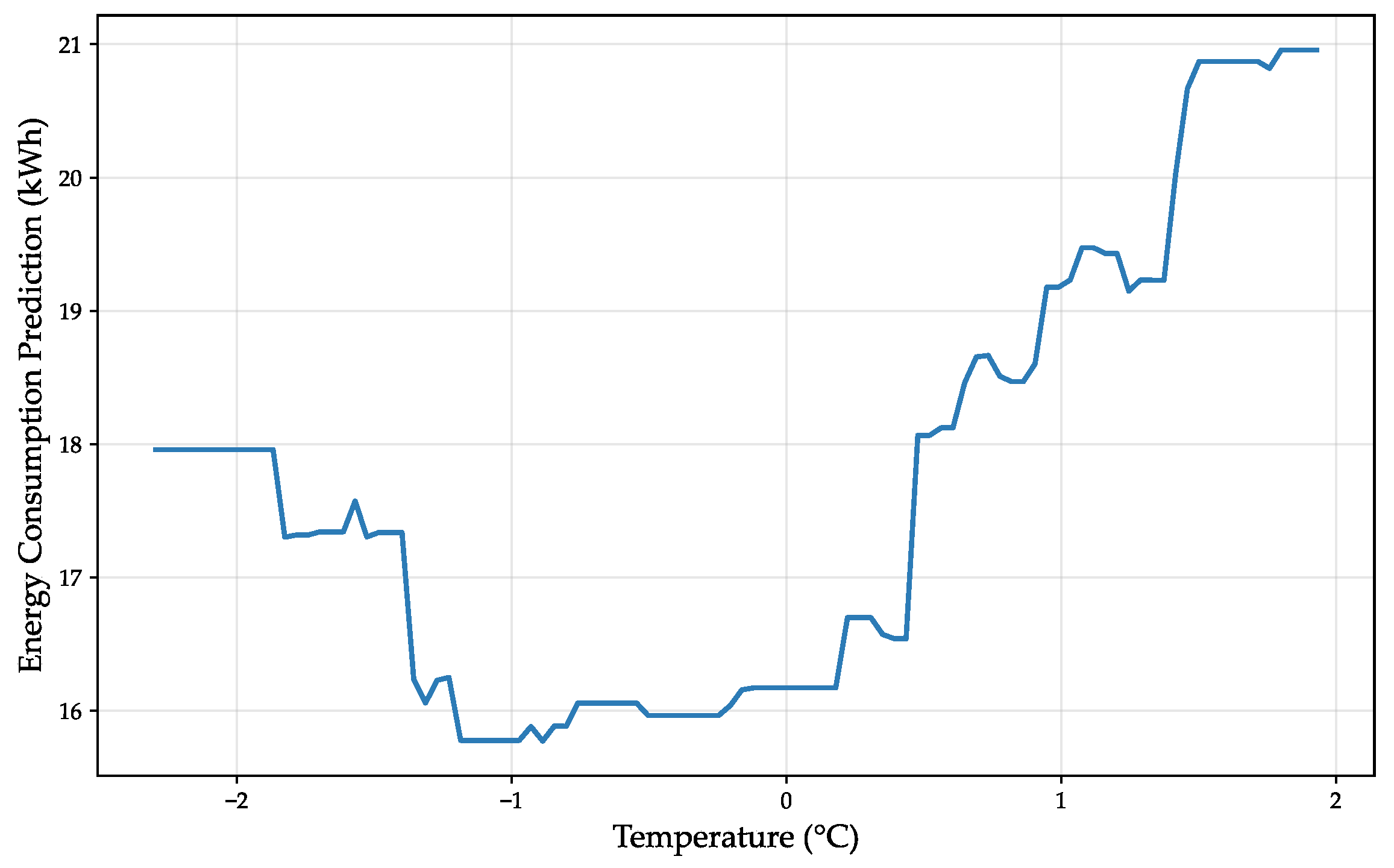
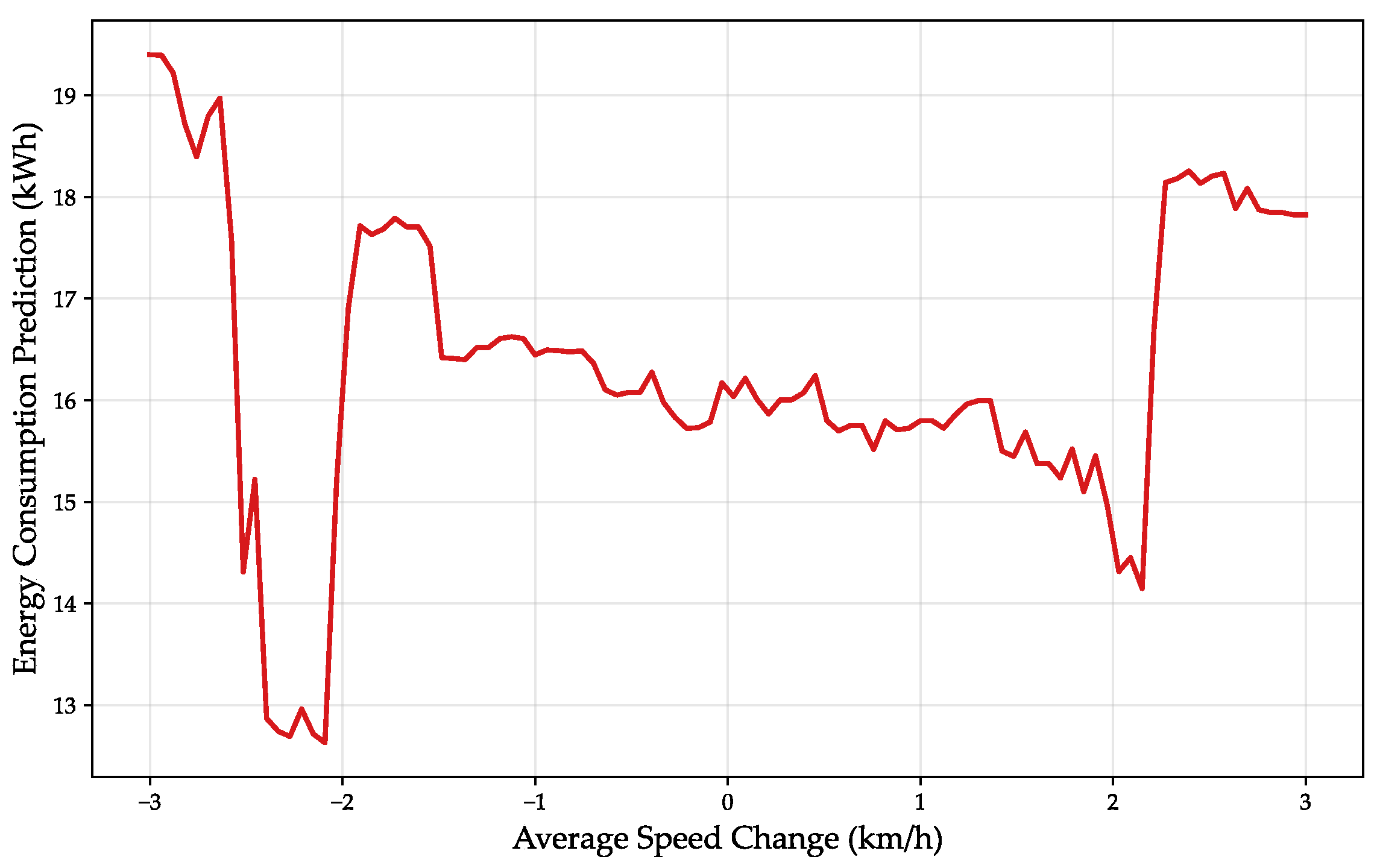
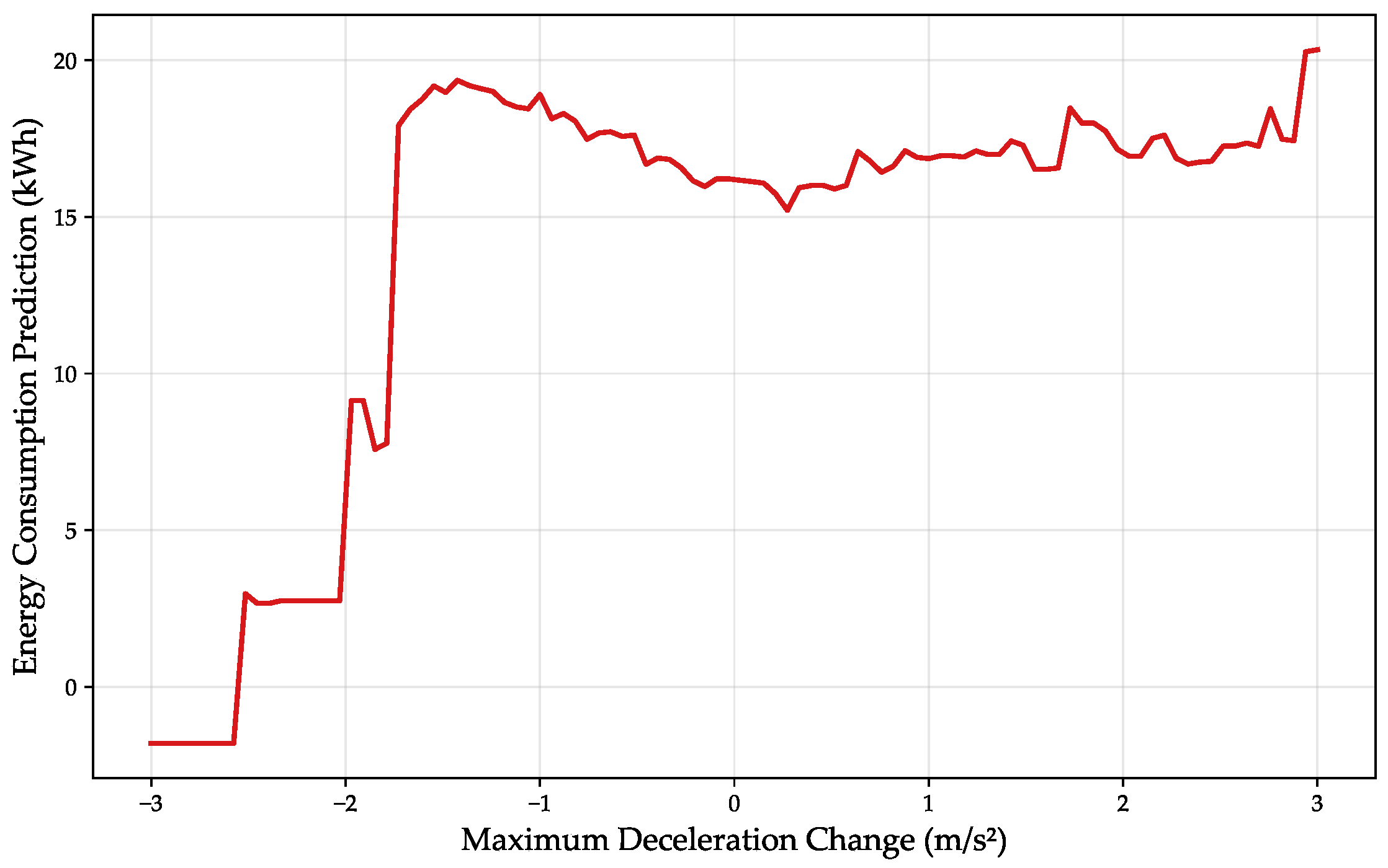
4.4. Sensitivity Analysis

To gain deeper insights into how various features influence EBs’ trip energy consumption, we conducted sensitivity analysis on key features identified through SHAP analysis. This analysis examined the impact of individual feature variations on trip-level energy consumption predictions while maintaining other features at their mean values. It’s important to note that only values near the baseline have practical significance.

The baseline values were established by calculating the mean of each feature in the training dataset, as shown in

Table 9. Baseline values for sensitivity analysis.

Parameter	Value
Temperature	24.76 °C
Average Speed	57.42 km/h
Maximum Deceleration	−1.38 m/s2

:

Temperature, as a crucial environmental factor, significantly affects trip-level energy consumption of EBs. As shown in Figure 18, with a baseline temperature of 24.76 °C, trip-level energy consumption exhibits nonlinear trends as the standardized temperature varies from minimum to maximum. In the low-temperature range (standardized value < −1), energy consumption decreases notably with rising temperature. In the moderate temperature range (−1 to 1), energy consumption remains relatively stable, indicating minimal temperature impact. In the high-temperature range (>1), energy consumption increases again, primarily due to increased air conditioning system load.

For driving behavior analysis, we selected the average speed and Maximum Deceleration as representative features based on SHAP analysis results. The analysis revealed the following insights:

• Impact of Average Speed;

As shown in Figure 19, there is a clear nonlinear relationship between average speed and trip-level energy consumption. With a baseline speed of 57.42 km/h, the low-speed range lacks explanatory power for trip-level energy prediction. In the baseline speed range [−2, +2], trip-level energy consumption decreases as speed increases, possibly due to reduced frequent stops and more stable operation, leading to lower energy losses from acceleration and braking. At medium to high speeds, energy consumption increases with speed, consistent with the physical principle of increasing air resistance.

2.

Impact of Maximum Deceleration;

As shown in Figure 20, the Maximum Deceleration’s impact on trip-level energy consumption shows a complex pattern. While the low deceleration range lacks practical significance, moderate deceleration contributes to energy recovery. Excessive deceleration may lead to increased energy loss as the regenerative braking system cannot engage effectively, forcing the mechanical brakes to engage and dissipate energy as heat.

These sensitivity analysis findings reveal the nonlinear relationships between environmental, operational factors, and trip-level energy consumption, providing practical guidance for EBs operation optimization in terms of HVAC management, driving strategy, and regenerative braking utilization.

5. Conclusions

This study presents a comprehensive approach to high-precision trip-level energy consumption prediction for EBs. The research advances existing methodologies by integrating detailed transmission system efficiency evaluation, dynamic passenger load estimation, and comprehensive feature incorporation spanning temporal, weather, and driving pattern characteristics. The LightGBM model demonstrated superior predictive performance while maintaining computational efficiency suitable for real-time IoT applications. Through SHAP and sensitivity analyses, we derived practical insights for optimizing EB operations. The resulting accurate trip-level energy consumption estimates serve as valuable parameters for subsequent optimization models [98], offering a deployable tool for enhancing EBs’ energy management systems.

The limitations of this study should also be acknowledged.

• Firstly, the traction modeling component lacks validation through actual experiments, which could further refine its accuracy.
• Secondly, the absence of detailed terrain data, such as slopes and curves, limits the model’s ability to fully capture the complexities of real-world routes, as it primarily focuses on relatively flat road segments.
• Thirdly, given that the studied vehicles were of similar condition and efficiency, the research may not have fully demonstrated the value of incorporating efficiency considerations under more diverse operational scenarios.

While this study validates the proposed framework through model comparisons and a physics-aligned design, future research will address existing limitations by incorporating field validations to achieve more precise model calibration. Further investigations will involve co-simulation with commercial platforms (e.g., AVL CRUISE) in scenarios where high-resolution road topology and motor efficiency data are accessible. Future research will also explore the model’s adaptability across diverse operating environments and examine its long-term performance in dynamic urban settings, aiming to enhance its robustness and applicability in broader contexts.

References

1. Manzolli, J.A.; Trovão, J.P.; Antunes, C.H. A review of electric bus vehicles research topics—Methods and trends. Renew. Sustain. Energy Rev. 2022, 159, 112211. [Google Scholar] [CrossRef]
2. Gao, H.; Liu, K.; Yao, E. Formation and scheduling optimization of electric modular buses with station-based demand-responsive model. China J. Highw. Transp. 2024, 37, 24–36. [Google Scholar] [CrossRef]
3. Gao, H.; Liu, K.; Wang, J.; Guo, F. Modular bus unit scheduling for an autonomous transit system under range and charging constraints. Appl. Sci. 2023, 13, 7661. [Google Scholar] [CrossRef]
4. Wang, J.; Zhang, Y.; Xing, X.; Zhan, Y.; Chan, W.K.V.; Tiwari, S. A data-driven system for cooperative-bus route planning based on generative adversarial network and metric learning. Ann. Oper. Res. 2024, 339, 427–453. [Google Scholar] [CrossRef]
5. IEA. Global EV Outlook 2024; IEA: Paris, France, 2024. [Google Scholar]
6. Wang, X.; Liu, W.; Zhang, L.; Zhang, M. CO2 emission reduction effect of electric bus based on energy chain in life cycle. J. Transp. Syst. Eng. Inf. Technol. 2019, 19, 19–25. [Google Scholar]
7. He, J.; Yan, N.; Zhang, J.; Wang, T.; Chen, Y.Y.; Tang, T.Q. Battery electricity bus charging schedule considering bus journey’s energy consumption estimation. Transp. Res. Part D Transp. Environ. 2023, 115, 103587. [Google Scholar] [CrossRef]
8. Berk Saner, C.; Trivedi, A.; Srinivasan, D. A multi-module modeling and optimization framework for integrated planning and operation of electric bus shuttle fleets. IEEE Trans. Intell. Transp. Syst. 2024, 25, 16910–16924. [Google Scholar] [CrossRef]
9. Liu, X.; Qu, X.; Ma, X. Optimizing electric bus charging infrastructure considering power matching and seasonality. Transp. Res. Part D Transp. Environ. 2021, 100, 103057. [Google Scholar] [CrossRef]
10. Shi, J.; Zhang, W.; Bao, Y.; Gao, D.W.; Fan, S. Game theory-based peer-to-peer energy storage sharing for multiple bus charging stations: A real-time distributed cooperative framework. J. Energy Storage 2025, 109, 115148. [Google Scholar] [CrossRef]
11. Liu, Z.; Ma, X.; Zhuo, S.; Liu, X. Optimizing shared charging services at sustainable bus charging hubs: A queue theory integration approach. Renew. Energy 2024, 237, 121860. [Google Scholar] [CrossRef]
12. Liu, K.; Wang, J.; Yamamoto, T.; Morikawa, T. Exploring the interactive effects of ambient temperature and vehicle auxiliary loads on electric vehicle energy consumption. Appl. Energy 2018, 227, 324–331. [Google Scholar] [CrossRef]
13. Gao, Y.; Guo, S.; Ren, J.; Zhao, Z.; Ehsan, A.; Zheng, Y. An electric bus power consumption model and optimization of charging scheduling concerning multi-external factors. Energies 2018, 11, 2060. [Google Scholar] [CrossRef]
14. Liu, K.; Gao, H.; Liang, Z.; Zhao, M.; Li, C. Optimal charging strategy for large-scale electric buses considering resource constraints. Transp. Res. Part D Transp. Environ. 2021, 99, 103009. [Google Scholar] [CrossRef]
15. Liu, K.; Gao, H.; Wang, Y.; Feng, T.; Li, C. Robust charging strategies for electric bus fleets under energy consumption uncertainty. Transp. Res. Part D Transp. Environ. 2022, 104, 103215. [Google Scholar] [CrossRef]
16. Chikishev, E. Impact of natural and climatic conditions on electric energy consumption by an electric city bus. Transp. Res. Procedia 2021, 57, 113–121. [Google Scholar] [CrossRef]
17. Li, M.; Yan, M.; He, H.; Peng, J. Data-driven predictive energy management and emission optimization for hybrid electric buses considering speed and passengers prediction. J. Clean. Prod. 2021, 304, 127139. [Google Scholar] [CrossRef]
18. Liu, K.; Wang, J.; Yamamoto, T.; Morikawa, T. Modelling the multilevel structure and mixed effects of the factors influencing the energy consumption of electric vehicles. Appl. Energy 2016, 183, 1351–1360. [Google Scholar] [CrossRef]
19. Galvin, R. Energy consumption effects of speed and acceleration in electric vehicles: Laboratory case studies and implications for drivers and policymakers. Transp. Res. Part D Transp. Environ. 2017, 53, 234–248. [Google Scholar] [CrossRef]
20. Hjelkrem, O.A.; Lervåg, K.Y.; Babri, S.; Lu, C.; Södersten, C.J. A battery electric bus energy consumption model for strategic purposes: Validation of a proposed model structure with data from bus fleets in China and Norway. Transp. Res. Part D Transp. Environ. 2021, 94, 102804. [Google Scholar] [CrossRef]
21. Ji, J.; Wang, L.; Bie, Y. Determination of GPS sampling interval for trip energy consumption estimation of electric buses: Analysis of real-world data. Proc. Inst. Mech. Eng. Part D J. Automob. Eng. 2024, 09544070241239384. [Google Scholar] [CrossRef]
22. Czapla, Z.; Sierpiński, G. Driving and energy profiles of urban bus routes predicted for operation with battery electric buses. Energies 2023, 16, 5706. [Google Scholar] [CrossRef]
23. Szilassy, P.Á.; Földes, D. Consumption estimation method for battery-electric buses using general line characteristics and temperature. Energy 2022, 261, 125080. [Google Scholar] [CrossRef]
24. Saadon Al-Ogaili, A.; Ramasamy, A.; Juhana Tengku Hashim, T.; Al-Masri, A.N.; Hoon, Y.; Neamah Jebur, M.; Verayiah, R.; Marsadek, M. Estimation of the energy consumption of battery driven electric buses by integrating digital elevation and longitudinal dynamic models: Malaysia as a case study. Appl. Energy 2020, 280, 115873. [Google Scholar] [CrossRef]
25. Li, X.; Wang, T.; Li, J.; Tian, Y.; Tian, J. Energy consumption estimation for electric buses based on a physical and data-driven fusion model. Energies 2022, 15, 4160. [Google Scholar] [CrossRef]
26. Zhou, X.; An, K.; Ma, W. Data-driven approach for estimating energy consumption of electric buses under on-road operation conditions. J. Transp. Eng. Part A Syst. 2023, 149, 04023089. [Google Scholar] [CrossRef]
27. Zhu, G.; Shi, M.; He, J. energy consumption prediction model for electric buses considering actual quantifiable features. J. Adv. Transp. 2024, 2024, 3058575. [Google Scholar] [CrossRef]
28. Sennefelder, R.M.; Martín-Clemente, R.; González-Carvajal, R. Energy consumption prediction of electric city buses using multiple linear regression. Energies 2023, 16, 4365. [Google Scholar] [CrossRef]
29. Blades, L.A.W.; Matthews, T.; McGrath, T.E.; Early, J.; Cunningham, G.; Harris, A. Predicting energy consumption of zero emission buses using route feature selection methods. Transp. Res. Part D Transp. Environ. 2024, 130, 104158. [Google Scholar] [CrossRef]
30. Qin, W.; Wang, L.; Liu, Y.; Xu, C. Energy consumption estimation of the electric bus based on grey wolf optimization algorithm and support vector machine regression. Sustainability 2021, 13, 4689. [Google Scholar] [CrossRef]
31. Hu, Z.; Zeng, X.; Feng, C.; Diao, H. optimizing charging and discharging at bus battery swap stations under varying environmental temperatures. Processes 2025, 13, 81. [Google Scholar] [CrossRef]
32. Zeng, Z.; Wang, T.; Qu, X. En-route charge scheduling for an electric bus network: Stochasticity and real-world practice. Transp. Res. Part E Logist. Transp. Rev. 2024, 185, 103498. [Google Scholar] [CrossRef]
33. Pan, Y.; Xi, Y.; Fang, W.; Liu, Y.; Zhang, Y.; Zhang, W. An eco-driving strategy for electric buses at signalized intersection with a bus stop based on energy consumption prediction. Energy 2025, 317, 134672. [Google Scholar] [CrossRef]
34. Zhang, Z.; Wang, S.; Ye, B.; Ma, Y. A feature prediction-based method for energy consumption prediction of electric buses. Energy 2025, 314, 134345. [Google Scholar] [CrossRef]
35. Xing, Y.; Li, Y.; Liu, W.; Li, W.; Meng, L. Operation energy consumption estimation method of electric bus based on CNN time series prediction. Math. Probl. Eng. 2022, 2022, 6904387. [Google Scholar] [CrossRef]
36. Pamuła, T.; Pamuła, D. Prediction of electric buses energy consumption from trip parameters using deep learning. Energies 2022, 15, 1747. [Google Scholar] [CrossRef]
37. Lin, M.; Chen, S.; Meng, J.; Wang, W.; Wu, J. Instantaneous energy consumption estimation for electric buses with a multi-model fusion method. IEEE Trans. Intell. Transp. Syst. 2025, 26, 371–381. [Google Scholar] [CrossRef]
38. Dong, C.; Xiong, Z.; Li, N.; Yu, X.; Liang, M.; Zhang, C.; Li, Y.; Wang, H. A real-time prediction framework for energy consumption of electric buses using integrated machine learning algorithms. Transp. Res. Part E Logist. Transp. Rev. 2025, 194, 103884. [Google Scholar] [CrossRef]
39. Xu, Z.; Wang, J.; Lund, P.D.; Zhang, Y. Analysis of energy consumption for electric buses based on low-frequency real-world data. Transp. Res. Part D Transp. Environ. 2023, 122, 103857. [Google Scholar] [CrossRef]
40. Chen, Y.; Zhang, Y.; Sun, R. Data-driven estimation of energy consumption for electric bus under real-world driving conditions. Transp. Res. Part D Transp. Environ. 2021, 98, 102969. [Google Scholar] [CrossRef]
41. Liu, Y.; Liang, H. A data-driven approach for electric bus energy consumption estimation. IEEE Trans. Intell. Transp. Syst. 2022, 23, 17027–17038. [Google Scholar] [CrossRef]
42. Smieszek, M.; Mateichyk, V.; Mosciszewski, J. The Influence of stops on the selected route of the city its on the energy efficiency of the public bus. Energies 2024, 17, 4179. [Google Scholar] [CrossRef]
43. Yi, F.; Guo, W.; Gong, H.; Shen, Y.; Zhou, J.; Yu, W.; Lu, D.; Jia, C.; Zhang, C.; Gong, F. Research on speed planning and energy management strategy for fuel cell hybrid bus in green wave scenarios at traffic light intersections based on deep reinforcement learning. Sustainability 2024, 16, 11156. [Google Scholar] [CrossRef]
44. Alarrouqi, R.A.; Ahmad, F.; Bayhan, S.; Al-Fagih, L. Electric buses in hot climates: Challenges, technologies, and the road ahead. IEEE Access 2024, 12, 55531–55550. [Google Scholar] [CrossRef]
45. Alarrouqi, R.A.; Bayhan, S.; Al-Fagih, L. An assessment of the energy performance of battery-electric buses in hot environments. Sustain. Energy Grids Netw. 2024, 38, 101352. [Google Scholar] [CrossRef]
46. Li, P.; Zhang, Y.; Zhang, Y.; Zhang, K.; Jiang, M. The effects of dynamic traffic conditions, route characteristics and environmental conditions on trip-based electricity consumption prediction of electric bus. Energy 2021, 218, 119437. [Google Scholar] [CrossRef]
47. Abdelaty, H.; Mohamed, M. A Prediction model for battery electric bus energy consumption in transit. Energies 2021, 14, 2824. [Google Scholar] [CrossRef]
48. Viana-Fons, J.D.; Payá, J. HVAC system operation, consumption and compressor size optimization in urban buses of Mediterranean cities. Energy 2024, 296, 131151. [Google Scholar] [CrossRef]
49. Zhao, L.; Li, Y.; Li, S.; Ke, H. A frequency item mining based embedded feature selection algorithm and its application in energy consumption prediction of electric bus. Energy 2023, 271, 126999. [Google Scholar] [CrossRef]
50. Li, P.; Zhang, Y.; Zhang, Y.; Zhang, Y.; Zhang, K. Prediction of electric bus energy consumption with stochastic speed profile generation modelling and data driven method based on real-world big data. Appl. Energy 2021, 298, 117204. [Google Scholar] [CrossRef]
51. Corbet, S.; Larkin, C.; McCluskey, J. The influence of inclement weather on electric bus efficiency: Evidence from a developed European network. Case Stud. Transp. Policy 2023, 12, 100971. [Google Scholar] [CrossRef]
52. Feng, N.; Yong, J.; Zhan, Z. A direct multiple shooting method to improve vehicle handling and stability for four hub-wheel-drive electric vehicle during regenerative braking. Inst. Mech. Eng. Part D J. Automob. Eng. 2020, 234, 1047–1056. [Google Scholar] [CrossRef]
53. Takeno, M.; Ogasawara, S.; Chiba, A.; Takemoto, M.; Hoshi, N. Power and efficiency measurements and design improvement of a 50 kW switched reluctance motor for hybrid electric vehicles. In Proceedings of the 2011 IEEE Energy Conversion Congress and Exposition, Phoenix, AZ, USA, 17–22 September 2011; pp. 1495–1501. [Google Scholar]
54. Roshandel, E.; Mahmoudi, A.; Kahourzade, S.; Yazdani, A.; Shafiullah, G.M. Losses in efficiency maps of electric vehicles: An overview. Energies 2021, 14, 7805. [Google Scholar] [CrossRef]
55. Zhang, Z.; Ye, B.; Wang, S.; Ma, Y. Analysis and estimation of energy consumption of electric buses using real-world data. Transp. Res. Part D Transp. Environ. 2024, 126, 104017. [Google Scholar] [CrossRef]
56. Zhang, Z.; Wang, S.; Lin, N.; Wang, Z.; Liu, P. State of health estimation of lithium-ion batteries in electric vehicles based on regional capacity and LGBM. Sustainability 2023, 15, 2052. [Google Scholar] [CrossRef]
57. She, C.; Zhang, Z.; Liu, P.; Sun, F. Overview of the application of big data analysis technology in new energy vehicle industry: Based on operating big data of new energy vehicle. J. Mech. Eng. 2019, 55, 3–16. [Google Scholar]
58. Li, F.; Min, Y.; Zhang, Y. Review of key technology research on the reliability of power lithium batteries based on big data. Energy Storage Sci. Technol. 2023, 12, 1981–1994. [Google Scholar]
59. Li, S.; He, H.; Zhao, P.; Cheng, S. Data cleaning and restoring method for vehicle battery big data platform. Appl. Energy 2022, 320, 119292. [Google Scholar] [CrossRef]
60. Sun, Z.; Wang, Z.; Chen, Y.; Liu, P.; Wang, S.; Zhang, Z.; Dorrell, D.G. Modified relative entropy-based lithium-ion battery pack online short-circuit detection for electric vehicle. IEEE Trans. Transp. Electrif. 2022, 8, 1710–1723. [Google Scholar] [CrossRef]
61. Hou, Y.; Zhang, Z.; Liu, P.; Song, C.; Wang, Z. Research on a novel data-driven aging estimation method for battery systems in real-world electric vehicles. Adv. Mech. Eng. 2021, 13, 16878140211027735. [Google Scholar] [CrossRef]
62. Huo, Q.; Ma, Z.; Zhao, X.; Zhang, T.; Zhang, Y. Bayesian network based state-of-health estimation for battery on electric vehicle application and its validation through real-world data. IEEE Access 2021, 9, 11328–11341. [Google Scholar] [CrossRef]
63. Li, S.; He, H.; Li, J. Big data driven lithium-ion battery modeling method based on SDAE-ELM algorithm and data pre-processing technology. Appl. Energy 2019, 242, 1259–1273. [Google Scholar] [CrossRef]
64. Wang, T.; Jing, Z.; Zhang, S.; Qiu, C. Utilizing principal component analysis and hierarchical clustering to develop driving cycles: A case study in Zhenjiang. Sustainability 2023, 15, 4845. [Google Scholar] [CrossRef]
65. Yu, H.; Liu, Y.; Zhang, H.; Li, J.; Liu, H. Impact of driving and driver’s operating characteristics on high fuel consumption set based on real-road driving data. Inst. Mech. Eng. Part D J. Automob. Eng. 2024, 238, 1455–1466. [Google Scholar] [CrossRef]
66. Wang, W.; Gao, G.; Wang, Z.; Liang, Y. A Method for Constructing Automobile Operation Condition. J. Highw. Transp. Res. Dev. 2020, 37, 128–138. [Google Scholar] [CrossRef]
67. Cao, Q.; Li, J.; Qu, D. Construction of Typical Driving Cycle for Passenger Cars in the City of Dalian. J. Shanghai Jiaotong Univ. 2018, 52, 1537–1542. [Google Scholar]
68. Rahimi-Eichi, H.; Ojha, U.; Baronti, F.; Chow, M.-Y. Battery Management System: An Overview of Its Application in the Smart Grid and Electric Vehicles. IEEE Ind. Electron. Mag. 2013, 7, 4–16. [Google Scholar] [CrossRef]
69. Zheng, F.; Jiang, J.; Sun, B.; Zhang, W.; Pecht, M. Temperature Dependent Power Capability Estimation of Lithium-Ion Batteries for Hybrid Electric Vehicles. Energy 2016, 113, 64–75. [Google Scholar] [CrossRef]
70. Bianchi, E.L.; Polinder, H.; Bandyopadhyay, S. Energy consumption of electric powertrain architectures: A comparative study. In Proceedings of the 2017 19th European Conference on Power Electronics and Applications (EPE’17 ECCE Europe), Warsaw, Poland, 11–14 September 2017; pp. P.1–P.10. [Google Scholar]
71. Lajunen, A.; Kalttonen, A. Investigation of thermal energy losses in the powertrain of an electric city bus. In Proceedings of the 2015 IEEE Transportation Electrification Conference and Expo (ITEC), Chennai, India, 27–29 August 2015; pp. 1–6. [Google Scholar]
72. Moein Jahromi, M.; Heidary, H. Chapter 14—Automotive applications of PEM technology. In PEM Fuel Cells; Kaur, G., Ed.; Elsevier: Amsterdam, The Netherlands, 2022; pp. 347–405. ISBN 978-0-12-823708-3. [Google Scholar]
73. Meißner, M.; Massalski, L. Modeling the electrical power and energy consumption of automated guided vehicles to improve the energy efficiency of production systems. Int. J. Adv. Manuf. Technol. 2020, 110, 481–498. [Google Scholar] [CrossRef]
74. Ji, J.; Bie, Y.; Zeng, Z.; Wang, L. Trip energy consumption estimation for electric buses. Commun. Transp. Res. 2022, 2, 100069. [Google Scholar] [CrossRef]
75. Kamran, M. Chapter 10—Electric vehicles and smart grids. In Fundamentals of Smart Grid Systems; Kamran, M., Ed.; Academic Press: Cambridge, MA, USA, 2023; pp. 431–460. ISBN 978-0-323-99560-3. [Google Scholar]
76. Yang, Y.; Gao, K.; Cui, S.; Xue, Y.; Najafi, A.; Andric, J. Data-driven rolling eco-speed optimization for autonomous vehicles. Front. Eng. Manag. 2024, 11, 620–632. [Google Scholar] [CrossRef]
77. Ni, D. Chapter 20—Vehicle Modeling. In Traffic Flow Theory; Ni, D., Ed.; Butterworth-Heinemann: Oxford, UK, 2016; pp. 279–285. ISBN 978-0-12-804134-5. [Google Scholar]
78. Ke, G.; Meng, Q.; Finley, T.; Wang, T.; Chen, W.; Ma, W.; Ye, Q.; Liu, T.Y. LightGBM: A highly efficient gradient boosting decision tree. In Proceedings of the Advances in Neural Information Processing Systems; Guyon, I., Luxburg, U.V., Bengio, S., Wallach, H., Fergus, R., Vishwanathan, S., Garnett, R., Eds.; Curran Associates, Inc.: Newry, Ireland, 2017; Volume 30. [Google Scholar]
79. Friedman, J.H. Greedy function approximation: A gradient boosting machine. Ann. Stat. 2001, 29, 1189–1232. [Google Scholar] [CrossRef]
80. Hochachka, W.M.; Caruana, R.; Fink, D.; Munson, A.; Riedewald, M.; Sorokina, D.; Kelling, S. Data-mining discovery of pattern and process in ecological systems. J. Wildl. Manag. 2007, 71, 2427–2437. [Google Scholar] [CrossRef]
81. Zhou, B.; Xu, J.; Han, F.; Yan, F.; Peng, S.; Li, Q.; Jiao, F. Pressure of different gases injected into large-scale coal matrix: Analysis of time–space dependence and prediction using light gradient boosting machine. Fuel 2020, 279, 118448. [Google Scholar] [CrossRef]
82. Zhong, Z.; Li, Y.; Han, Z.; Yang, Z. Ship target detection based on LightGBM algorithm. In Proceedings of the 2020 International Conference on Computer Information and Big Data Applications (CIBDA), Guiyang, China, 17–19 April 2020; pp. 425–429. [Google Scholar]
83. Yin, L.; Ma, P.; Deng, Z. JLGBMLoc—A novel high-precision indoor localization method based on LightGBM. Sensors 2021, 21, 2722. [Google Scholar] [CrossRef]
84. Liang, W.; Luo, S.; Zhao, G.; Wu, H. Predicting hard rock pillar stability using GBDT, XGBoost, and LightGBM algorithms. Mathematics 2020, 8, 765. [Google Scholar] [CrossRef]
85. Massaoudi, M.; Refaat, S.S.; Chihi, I.; Trabelsi, M.; Oueslati, F.S.; Abu-Rub, H. A novel stacked generalization ensemble-based hybrid lgbm-xgb-mlp model for short-term load forecasting. Energy 2021, 214, 118874. [Google Scholar] [CrossRef]
86. Gan, M.; Pan, S.; Chen, Y.; Cheng, C.; Pan, H.; Zhu, X. Application of the machine learning LightGBM model to the prediction of the water levels of the lower Columbia river. J. Mar. Sci. Eng. 2021, 9, 496. [Google Scholar] [CrossRef]
87. Wang, Y.; Wang, T. Application of improved LightGBM model in blood glucose prediction. Appl. Sci. 2020, 10, 3227. [Google Scholar] [CrossRef]
88. Jabeur, S.B.; Gharib, C.; Mefteh-Wali, S.; Arfi, W.B. CatBoost model and artificial intelligence techniques for corporate failure prediction. Technol. Forecast. Soc. Change 2021, 166, 120658. [Google Scholar] [CrossRef]
89. Fu, X.Y.; Mao, X.L.; Wu, H.W.; Lin, J.Y.; Ma, Z.Q.; Liu, Z.C.; Cai, Y.; Yan, L.L.; Sun, Y.; Ye, L.P.; et al. Development and validation of LightGBM algorithm for optimizing of helicobacter pylori antibody during the minimum living guarantee crowd based gastric cancer screening program in Taizhou, China. Prev. Med. 2023, 174, 107605. [Google Scholar] [CrossRef]
90. Jiao, S.; Zou, Q. Identification of plant vacuole proteins by exploiting deep representation learning features. Comput. Struct. Biotechnol. J. 2022, 20, 2921–2927. [Google Scholar] [CrossRef] [PubMed]
91. Svetnik, V.; Liaw, A.; Tong, C.; Wang, T. Application of breiman’s random forest to modeling structure-activity relationships of pharmaceutical molecules. In Proceedings of the Multiple Classifier Systems, Cagliari, Italy, 9–11 June 2004; Roli, F., Kittler, J., Windeatt, T., Eds.; Springer: Berlin/Heidelberg, Germany, 2004; pp. 334–343. [Google Scholar]
92. Frazier, P.I. A Tutorial on bayesian optimization. arXiv 2018, arXiv:1807.02811. [Google Scholar] [CrossRef]
93. Morita, Y.; Rezaeiravesh, S.; Tabatabaei, N.; Vinuesa, R.; Fukagata, K.; Schlatter, P. Applying bayesian optimization with gaussian process regression to computational fluid dynamics problems. J. Comput. Phys. 2022, 449, 110788. [Google Scholar] [CrossRef]
94. Microsoft Corporation Parameters Tuning. Available online: https://lightgbm.readthedocs.io/en/latest/Parameters-Tuning.html (accessed on 16 February 2025).
95. Van Hoof, J.; Vanschoren, J. Hyperboost: Hyperparameter Optimization by Gradient Boosting surrogate models. arXiv 2021, arXiv:2101.02289. [Google Scholar] [CrossRef]
96. Lundberg, S.; Lee, S.I. A Unified Approach to Interpreting Model Predictions. arXiv 2017, arXiv:1705.07874. [Google Scholar] [CrossRef]
97. Takeishi, N. Shapley values of reconstruction errors of pca for explaining anomaly detection. In Proceedings of the 2019 International Conference on Data Mining Workshops (ICDMW), Beijing, China, 8–9 November 2019; pp. 793–798. [Google Scholar]
98. Zhong, L.; Zeng, Z.; Huang, Z.; Shi, X.; Bie, Y. Joint optimization of electric bus charging and energy storage system scheduling. Front. Eng. Manag. 2024, 11, 676–696. [Google Scholar] [CrossRef]
Figure 1. Altitude changes from start to end stations.
Wevj 16 00159 g001
Figure 2. GPS trajectory and heatmap visualization.
Wevj 16 00159 g002
Figure 3. Distribution of voltage values.
Wevj 16 00159 g003
Figure 4. IQR multiplier vs. detected outliers.
Wevj 16 00159 g004
Figure 5. Daily segmentation of discharge cycle into trips.
Wevj 16 00159 g005
Figure 6. Scree plot of PCA features.
Wevj 16 00159 g006
Figure 7. Diagram of brake energy regeneration process.
Wevj 16 00159 g007
Figure 8. Diagram of energy transfer chain.
Wevj 16 00159 g008
Figure 9. Diagram of histogram algorithm.
Wevj 16 00159 g009
Figure 10. Comparison of leaf-wise and level-wise tree growth strategies.
Wevj 16 00159 g010
Figure 11. Framework of model construction.
Wevj 16 00159 g011
Figure 12. Dataset splitting and 5-fold cross-validation.
Wevj 16 00159 g012
Figure 13. Bayesian Optimization convergence.
Wevj 16 00159 g013
Figure 14. Absolute error for the test dataset.
Wevj 16 00159 g014
Figure 15. Error percentages across different models.
Wevj 16 00159 g015
Figure 16. SHAP effects distribution (red for high values and blue for low values).
Wevj 16 00159 g016
Figure 17. Mean absolute SHAP value of decomposed driving characteristics.
Wevj 16 00159 g017
Figure 18. Temperature Sensitivity Analysis.
Wevj 16 00159 g018
Figure 19. Average speed sensitivity analysis.
Wevj 16 00159 g019
Figure 20. Maximum deceleration sensitivity analysis.
Wevj 16 00159 g020