Generating Realistic Vehicle Trajectories Based on Vehicle–Vehicle and Vehicle–Map Interaction Pattern Learning

Abstract

Diversified and realistic traffic scenarios are a crucial foundation for evaluating the safety of autonomous driving systems in simulations. However, a considerable number of current methods generate scenarios that lack sufficient realism. To address this issue, this paper proposes a vehicle trajectory generation method based on vehicle–vehicle and vehicle–map interaction pattern learning. By leveraging a multihead self-attention mechanism, the model efficiently captures complex dependencies among vehicles, enhancing its ability to learn realistic traffic dynamics. Moreover, the multihead cross-attention mechanism is also used to learn the interaction features between the vehicles and the map, addressing the challenge of trajectory generation’s difficulty in perceiving static environments. This proposed method enhances the model’s ability to learn natural traffic sequences, enable the generation of more realistic traffic flow, and provide strong support for the testing and optimization of autonomous driving systems. Experimental results show that compared to the Trafficgen baseline model, the proposed method achieves a 26% improvement in ADE and a 20% improvement in FDE.

1. Introduction

Autonomous driving (AD) is expected to prevent road accidents and save millions of lives while also improving the livelihoods and quality of life for many people. However, there is still much work to be undertaken to develop a system that can operate at a level comparable to the best human drivers. One of the main challenges in deploying autonomous driving in the real world is ensuring that algorithm-controlled vehicles can operate safely and reliably in diverse traffic scenarios. Simulation environments provide a controlled, repeatable, and low-risk testing ground for autonomous driving algorithms, where developers can simulate various traffic situations and conduct tests under extreme conditions. Most existing simulators, such as CARLA [1], SMARTS [2], and SUMO [3], still have some limitations. The traffic flow generation rules in these simulation systems are typically manually added, such as lane following and mutual detection and avoidance between vehicles and pedestrians. These rules lack sufficient flexibility and diversity, preventing the system from reproducing the complex traffic behaviors and natural variations found in the real world, such as overtaking and lane changing.

Moreover, the evaluation of the reliability of autonomous driving systems in simulation environments relies heavily on large amounts of real-world datasets. Acquiring these datasets for natural scenarios requires significant manual collection and annotation costs. Even existing datasets typically represent only fragments of scenes, with most lasting for a very short time, and traffic participants are sometimes obscured. For example, in the Waymo Motion dataset [4], only 30% of the trajectories last longer than 10 s, and only 12% of the trajectories cover the entire scene [5]. These available scenarios and their levels of complexity are far from sufficient to meet the requirements for reliably evaluating autonomous driving systems. Consequently, it remains challenging to assess how autonomous driving systems can make safety-critical decisions and respond to other traffic participants in complex traffic scenarios. Therefore, creating diverse and realistic traffic scenarios in simulations is essential for thoroughly evaluating the AI safety of autonomous driving systems.

Simulating the real world for autonomous vehicles remains an open challenge. Changing the state of one traffic participant requires other participants to make corresponding reactions. These reactions must align with the patterns observed in natural scenes, which is a problem that cannot be solved by manual additions. To address this challenge, we propose a model that can learn traffic flow from natural scenes: a trajectory generation model based on vehicle–vehicle interaction and vehicle–map interaction. This model is capable of learning real and diverse traffic scene flows from the real world. After learning, given the initial state of the traffic scene flow, the model can continue to generate vehicle behaviors. If the traffic flow scenario is not rich enough, the model can also enhance the traffic flow scene through data augmentation. The generated traffic flow scenes provide rich and realistic data for safety testing of autonomous driving. The following are the contributions of our work:

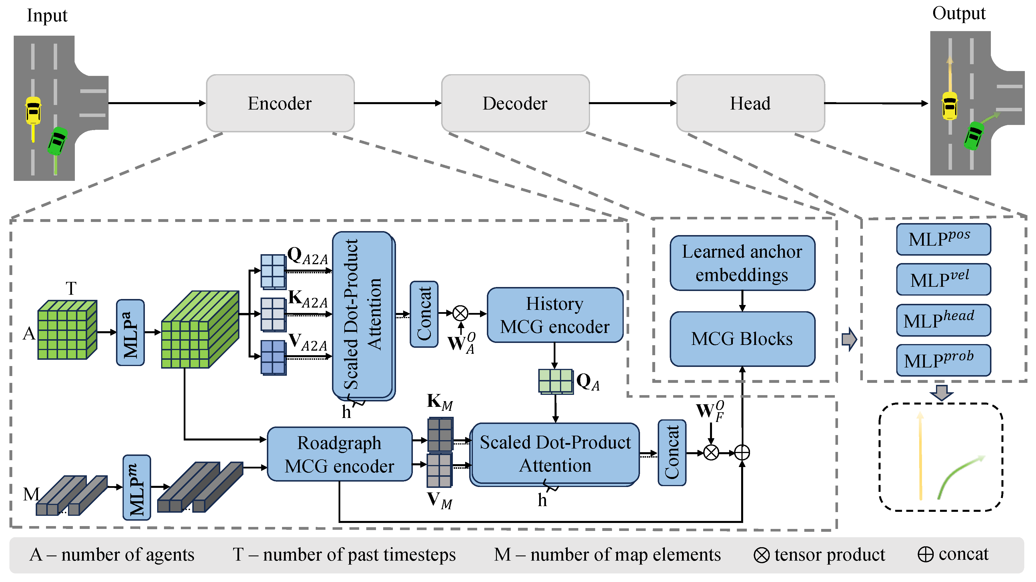
• The multihead self-attention module effectively captures intricate intervehicle dependencies by computing the influence each vehicle has on others. This allows the model to understand how each participant’s behavior is shaped by the surrounding vehicles. By modeling dynamic relationships such as mutual avoidance, following, and cooperation, this module significantly enhances the accuracy and reliability of trajectory generation.
• The multihead cross-attention module integrates map information with vehicle trajectories, addressing the challenge of incorporating static environmental constraints like road structures, landmark positions, and traffic rules. This module captures the geometric characteristics of the road, the impact of landmarks, and the influence of traffic rules, thereby improving the model’s adaptability in complex environments.

2. Related Work

Traffic flow simulation is a critical task, particularly in the development and testing of autonomous vehicles. By simulating traffic environments, autonomous driving algorithms can be trained and tested to ensure they can handle complex traffic scenarios safely and efficiently before real-world deployment [6].

In existing traffic simulations, most are based on real-world data collection records [7,8]. The open-source traffic simulator SUMO [3] is implemented based on a microscopic traffic flow model. Pérez et al. [9] used Bezier curves and spline curves for the trajectory generation of autonomous vehicles in urban environments, aiming for path smoothing and continuous curvature. Uhrmacher [10] made detailed improvements to these methods, enhancing the naturalness to some extent, but they still cannot fit the complex behaviors and interactions that occur in real-world situations. Furthermore, expanding these models requires substantial expertise and a significant amount of time. Gao et al. [11] proposed a real trajectory generation method based on dynamic deduction for a random microscopic traffic flow model. This study addressed the issue of unrealistic vehicle trajectory simulation in random microscopic traffic flow models, providing a more precise simulation environment for autonomous driving validation. Mullakkal-Babu et al. [12] introduced a submicroscopic–microscopic simulation framework incorporating vehicle lateral dynamics, solving the problem of unreasonable lateral motion in traditional microscopic models. This achieved more realistic lateral behavior simulation and unified the representation of macroscopic traffic flow phenomena. Dobrilko and Bublil [13] were able to reproduce real vehicle trajectories through simulation calibration (such as vehicle-following models and trajectory distributions), including the dynamic behavior of individual vehicles (such as acceleration, deceleration, and lane changes).

Some methods aim to learn the probabilistic distribution of traffic scenarios from sampled data [14,15,16,17]. For instance, Wheeler and Kochenderfer [15] proposed a scenario distribution modeling method for vehicle safety analysis, which uses factor graphs to construct scenario models. The method uses a factor graph to construct a scene model, accurately reflecting vehicle states and interrelations under different road structures, and effectively handles complex road network layouts. It is adaptable to diverse road layouts and can handle interlane relationships, which aligns with the frequent interactions in multilane urban traffic. Based on continuous feature descriptions of vehicle states, it avoids information loss and precisely reflects dynamic traffic changes. Additionally, the model is flexible for expansion, allowing the addition of variables and factors to adapt to the dynamic evolution of traffic scenarios. However, it only considers a limited set of road topologies, making it difficult to generalize to real urban scenarios, as these are far more complex and may not follow standard reference paths.

In recent years, with the rapid development of autonomous driving and the availability of extensive datasets [4,8,18], motion prediction models have also advanced significantly. These motion prediction models are now widely applied in traffic flow generation. Gao et al. [19], inspired by Natural Language Processing (NLP), proposed vector encoding for traffic flows and constructed a graph neural network-based architecture. By implementing attention mechanisms at both the node and global levels, their model achieved superior performance, with impressive results demonstrated on the Argoverse dataset and their internal dataset. Their structure is a variation of PointNet. The Trafficsim [20] model leverages the latest advancements in trajectory prediction and employs an implicit latent variable model to formulate joint actor policies, enabling the parallel generation of multiple consistent actor trajectory samples across scenarios. Scene Transformer [21] is also inspired by NLP and consists of three stages: embedding, encoding, and decoding. It adopts a scene-centered representation. During the encoding phase, an attention-based network is used to capture dependencies between time, agents, and road graph elements by efficiently decomposing attention and cross-attention. The model aggregates displacement loss for backpropagation.

Currently, some researchers have made significant contributions to this field by implementing simulated traffic models with various networks. For instance, Suo et al. [20] and Rempe et al. [22] used Variational Autoencoder (VAE-type) generative models, while Igl et al. [23] achieved this task using generative adversarial networks. Zhong et al. [24] and Jiang et al. [25] utilized diffusion models for this purpose. Trajeglish [26] achieved efficient discretization through k-disks while maintaining a low error. The model significantly improved its ability to simulate traffic scenarios by integrating map information into the encoding process, a feature that played a key role in vehicle driving decision prediction. However, the model lost some details at high resolution for continuous states. Trafficgen [5] divided the task into two subtasks: vehicle placement and trajectory generation. Our work is largely built upon the latest models for traffic flow generation and incorporates the most recent advancements in trajectory prediction to improve trajectory generation models. The rest of this paper is organized as follows. Section 3 presents the proposed method, Section 4 gives the experiments, and Section 5 concludes this paper.

3. Our Method

In this section, we introduce the method, which is based on vehicle–vehicle and vehicle–map interactions. The structure of this network model is shown in Figure 1. It consists of three modules: an encoder module with interactions, a decoder module with interactions, and a head for generating trajectories. We provide a detailed description of our method below.

To evaluate our approach, we choose Trafficgen as the baseline model due to its ability to generate trajectories that closely resemble actual traffic patterns. However, we observed that Trafficgen sometimes struggles to generate realistic trajectories, especially over long distances. Motivated by these limitations, we propose an improved method that enhances the trajectory generation process, addressing the challenges faced by Trafficgen.

We use $\mathsf{\Psi }$ to represent the entire scenario, $\mathbf{m}$ to represent map information, T for the duration of the scenario, and $s_t,t\in \left[1,T\right]$ to denote the set of all vehicle states in the scenario at time t. The state of the j-th vehicle at time t is represented as $s_t^j,j\in [1,J]$. The state of each $s_t^j$ is represented using 7 dimensions, which include position $p_x^j,p_y^j$, longitudinal and lateral velocity $v_x^j,v_y^j$, heading $h^j$, as well as length and width $box{l}^j,box{w}^j$. Similar to VectorNet encoding, we vectorize the elements of the map into a set of vectors, where each vector represents a part of the map. As shown in Figure 2, each vector contains a starting point ${\mathrm{d}}_i^s$ and an endpoint ${\mathrm{d}}_i^e$, where ${\mathrm{d}}_i^s,{\mathrm{d}}_i^e\in {\mathbb{R}}^2$. This is denoted as $c_i$. Based on these vectors, we establish a coordinate system in which vehicles are expressed.

To better facilitate interaction between the map and vehicles, we incorporate lane type ${type}_i$ and traffic signal information $g_i$ into these vectorized features. Therefore, at a given time t, the scene vector encoding for a specific vehicle is represented as ${\mathbf{v}}_t^j={\{c_i,typ{e}_i,g_i\}}_{i=1}^I\oplus (p_x^j,p_y^j,v_x^j,v_y^j,h^j,box{l}^j,box{w}^j)$, where ⊕ concatenates the map to the vehicle and I denotes the number of surrounding vectors. The information for scenario $\mathsf{\Psi }$ at time t is thus represented as ${\mathsf{\Psi }}_t={\left\{{\mathbf{v}}_t^j\right\}}_{j=1}^J$.

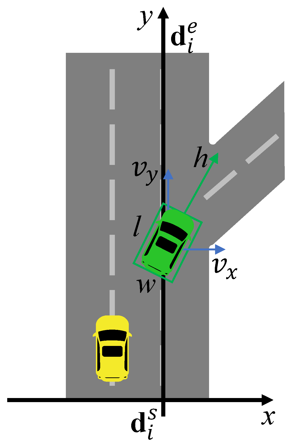
3.1. Multidimensional Vehicle Initial State Sampling

To ensure that our vehicle is closer to the traffic flow in a natural state, we need to encode the initial state of each traffic participant. This means we need to model the vehicle’s initialization and then learn the distribution relationships of the vehicles on the map in the natural state. Here, we use Trafficgen’s method to sample the state information of vehicles to determine where our vehicles should be placed. This method generates a set of weights for all regions to parameterize whether a vehicle should be placed in a particular area and to parameterize the vehicle category distribution. Specifically, we use a Multilayer Perceptron (MLP) to parameterize the categorical distribution and normal distribution. Using the parameterized categorical distribution and binary normal distribution, the vehicle placement information is determined as follows:

$${\omega }_j={\mathrm{MLP}}_{\mathrm{place}}\left(v_j^{\prime }\right)\forall j=1,\dots ,I,$$

(1)

$$i\sim \mathrm{Categorical}\left({[{\omega }_1,\dots ,{\omega }_I]}^{\mathrm{T}}\right),$$

(2)

where ${\mathbf{v}}^{\prime }$ represents the features output by the decoder module with feature fusion, $v_j^{\prime }$ is the feature of a specific region, and i is the selected region. We input this into the MLP network, which is used to model the distribution of vehicle attributes. For the vehicle’s position, we use a mixture of K binary normal distributions to model it:

$$[{\pi }_{\mathrm{pos}},{\mu }_{\mathrm{pos}},{\sum }_{\mathrm{pos}}]={\mathrm{MLP}}_{\mathrm{pos}}\left(v_i^{\prime }\right),$$

(3)

$$k\sim \mathrm{Categorical}\left({\pi }_{\mathrm{pos}}\right),$$

(4)

$$q_i\sim \mathrm{Normal}({\mu }_{pos,k},{\sigma }_{pos,k}),$$

(5)

where ${\mu }_{pos,k},{\sigma }_{pos,k}$ represent the mean vector and covariance matrix of the binary normal distribution and ${\pi }_{\mathrm{pos}}$ represents the weight of the K categorical distributions. Using this method, we can separately establish the mixture distributions for heading, speed, and vehicle size. This way, we provide the initial state for our subsequent trajectory generation tasks, allowing us to iteratively generate trajectory information.

3.2. Encoder Module

Here, we use an MLP to perform dimensional expansion of the agent and map vector information:

$$a_J^T=f_{mlp}\left([s_1^1,\dots ,s_T^1,s_1^2,\dots ,s_T^J]\right),$$

(6)

$$l=f_{mlp}\left([c_1,\dots ,c_I]\right)\oplus f_{Embedding}\left([typ{e}_1,\dots ,typ{e}_I]\right)\oplus f_{Embedding}\left([g_1,\dots ,g_I]\right)$$

(7)

We know that in natural conditions, there is interaction information between vehicles, so we need to model the interactions between them. In terms of global modeling capabilities, the self-attention mechanism has a clear advantage because it can explicitly capture the relationship between any two elements, allowing it to handle long-distance dependencies and global information. Inspired by trajectory prediction and the attention mechanism, we use the self-attention module to enhance the interaction information between vehicles.

$${\mathbf{Q}}_{A2A}={\mathbf{XW}}_{A2A}^Q,{\mathbf{K}}_{A2A}={\mathbf{XW}}_{A2A}^K,{\mathbf{V}}_{A2A}{=\mathbf{XW}}_{A2A}^V$$

(8)

Our input tensor is $\mathbf{X}\in {\mathbb{R}}^{B\times N\times d_{model}}$, and ${\mathbf{W}}_{A2A}^Q,{\mathbf{W}}_{A2A}^K,{\mathbf{W}}_{A2A}^V\in {\mathbb{R}}^{d_{model}\times d_k}$ is the weight matrix for the linear transformation. ${\mathbf{Q}}_{A2A},{\mathbf{K}}_{A2A},{\mathbf{V}}_{A2A}\in {\mathbb{R}}^{B\times N\times d_k}$ represents the resulting tensor. $e_i$ represents the attention score. For each head, we compute as follows:

$$\mathrm{Attention}({\mathbf{Q}}_{A2A},{\mathbf{K}}_{A2A},{\mathbf{V}}_{A2A})=\mathrm{Softmax}({\displaystyle \frac{{\mathbf{Q}}_{A2A}·{\mathbf{K}}_{A2A}^{\mathrm{T}}}{\sqrt{d_k}}}){\mathbf{V}}_{A2A}$$

(9)

$$\mathrm{Softmax}(e_i)={\displaystyle \frac{exp\left(e_i\right)}{{\sum }_{j=1}^{n}exp\left(e_j\right)}}\in (0,1)$$

(10)

We use h independent attention heads to compute for $\mathbf{Q},\mathbf{K}$, and $\mathbf{V}$ separately:

$${\mathrm{Head}}_i=\mathrm{Attention}({\mathbf{Q}}_{A2A}^i,{\mathbf{K}}_{A2A}^i,{\mathbf{V}}_{A2A}^i),i=1,2,\dots ,h$$

(11)

The output of each head is ${\mathrm{Head}}_i\in {\mathbb{R}}^{B\times N\times d_k}$. The results of all heads are concatenated along the last dimension:

$$\mathrm{MultiHead}({\mathbf{Q}}_{A2A},{\mathbf{K}}_{A2A},{\mathbf{V}}_{A2A})=\mathrm{Concat}({\mathrm{Head}}_1,\dots ,{\mathrm{Head}}_h){\mathbf{W}}_A^O$$

(12)

We use the Multicontext Gating (MCG) module [27] for context learning in the scene. This module addresses the weak interaction issue caused by independently encoding each element. Unlike attention mechanisms, which have high computational complexity, the MCG module—also known as the context gating module—is an efficient information fusion mechanism designed to integrate input encodings from different modalities. Within this framework, elements can access context vectors that depend on the encoding conditions. MCG is designed to effectively combine multimodal information in behavior prediction models, such as road elements, the historical states of agents, and interaction features. This can be viewed as an approximation of cross-attention. By introducing context vectors, MCG aggregates information from various input modalities.

$$\mathbf{A}={\mathrm{MCG}}_{history}(\mathbf{a}),\mathbf{M}={\mathrm{MCG}}_{\mathrm{road}}(l,\mathbf{a})$$

(13)

We know that vehicles driving on the road not only are interacting with surrounding vehicles but also are strongly correlated with map information. Obviously, traffic light states, lane line information, traffic signs, etc., all affect vehicle movement. In our previous encoding, the features can be divided into two types, map features and vehicle dynamic features, which together describe a traffic flow scene. Therefore, how to fuse these features is crucial. In this module, we optimize the feature fusion process. The fused features are concatenated with map features to serve as the features for the next layer. This is represented using the following formula:

$${\mathbf{Q}}_A={\mathbf{AW}}_A^Q\in {\mathbb{R}}^{B\times N\times d_k},{\mathbf{K}}_M={\mathbf{MW}}_M^K\in {\mathbb{R}}^{B\times 1\times d_k},{\mathbf{V}}_M={\mathbf{MW}}_M^V\in {\mathbb{R}}^{B\times 1\times d_k}$$

(14)

Here, $\mathbf{A}\in {\mathbb{R}}^{B\times N\times d_{model}},\mathbf{M}\in {\mathbb{R}}^{B\times d_{model}}$, where B is the batch size, N is the number of agents, and $d_{\mathrm{model}}$ is the feature dimension. The query vector comes from the agent features, while the keys and values come from the map features. ${\mathbf{W}}_A^Q\in {\mathbb{R}}^{d_{\mathrm{model}}\times d_k},{\mathbf{W}}_M^K\in {\mathbb{R}}^{d_{\mathrm{model}}\times d_k},{\mathbf{W}}_M^V\in {\mathbb{R}}^{d_{\mathrm{model}}\times d_k}$ are the linear transformation matrices for the query, key, and value, respectively. This design ensures that vehicle states are updated dynamically based on static map constraints. The calculation process is similar to the self-attention mechanism described above, so it will not be elaborated further. Through the above interactions, the final result obtained is concatenated with $\mathbf{M}$ to generate the final ${\mathbf{F}}_{fusion}$.

3.3. Decoder Module

To effectively guide the model in generating trajectories with controlled behavior, anchor point information is added. Using anchor points can effectively mitigate the mode collapse problem, resulting in more robust and interpretable trajectories.

$$\mathbf{F}={\mathrm{MCG}}_{blocks}({\mathbf{F}}_{fusion},anchor)$$

(15)

3.4. Head

After obtaining the features from the decoder’s output, we use multiple three-layer MLPs to output the trajectory information of our vehicle, where $prob$ represents the probability distribution of the trajectory, $v_x,v_y,p_x,p_y$ represent the lateral and longitudinal speed and position of the vehicle, and h denotes the heading. The details are as follows:

$$prob,v_x,v_y,p_x,p_y,h=\mathrm{MLPs}\left(\mathbf{F}\right)$$

(16)

3.5. Loss Function

Our model produces multimodal outputs, generating six modalities for a single trajectory. The position loss and velocity loss are calculated using the Mean Squared Error (MSE) function, and their average is computed using the mean. The difference between the generated probability distribution and the target position with the minimum distance is calculated using the Cross-Entropy loss. The average absolute error between the generated heading and the true heading is computed using the L1 norm loss function. The specific equations are as follows:

$$\mathrm{pos\_loss}=\mathrm{mean}\left(\mathrm{MSE}\right(p_x,p_y,p_x^{gt},p_y^{gt}\left)\right)$$

(17)

$$\mathrm{velo\_loss}=\mathrm{mean}(\mathrm{MSE}(v_x,v_y,v_x^{gt},v_y^{gt}\left)\right)$$

(18)

$$\mathrm{cls\_loss}=\mathrm{CrossEntropyLoss}(prob,{prob}_{min})$$

(19)

$$\mathrm{heading\_loss}=\mathrm{mean}(\mathrm{L}1(h,h^{gt}))$$

(20)

$$\mathrm{loss\_sum}=\mathrm{pos\_loss}+\mathrm{velo\_loss}+\mathrm{heading\_loss}+\mathrm{cls\_loss}$$

(21)

4. Experiment

4.1. Datasets and Experimental Setting

We trained our model using the Waymo Motion dataset [4], which contains approximately 70,000 scenes, including a mix of road segments and intersections, with a total duration of about 574 h. The sampling frequency is 10 Hz, and each scene includes a 20-second trajectory. This dataset also contains rich information, such as traffic signal state information, vehicle length and width details, and more. During training, we used data from the first 9 s as the training input. The map data range was limited to 60 m, and the road sampling rate was set to 10. We used 70,000 scenes for training, with each scene sampling up to 32 agents. The feature size of the model was set to 1024. The proposed method was implemented using the PyTorch framework (version 2.1.2+cu118), and all networks were trained on two NVIDIA GTX 3090 GPUs (manufactured by NVIDIA Corporation, Santa Clara, CA, USA). The model was trained for 100 epochs, with an initial learning rate of $2\times {10}^{-3}$, and we utilized the Distributed Data Parallelism (DDP) strategy to efficiently leverage multiple GPUs or nodes during training. For comparison, we chose Trafficgen as the baseline model.

In addition, we further conducted comparative experiments by degenerating the model into a trajectory prediction model and testing it on the Argoverse dataset [8].

4.2. Evaluation Metrics

The following metrics were used to evaluate the performance of the proposed method:

• Average Displacement Error (ADE): The average Euclidean distance (in meters) between the predicted trajectory and the ground-truth trajectory across all time points.
• Final Displacement Error (FDE): The Euclidean distance (in meters) between the predicted trajectory’s final time point and the ground-truth trajectory’s final time point.
• Minimum Average Displacement Error (minADE): The average L2 distance (in meters) between the best forecasted trajectory and the ground truth. The best here refers to the trajectory that has the minimum endpoint error.
• Minimum Final Displacement Error (minFDE): The L2 distance (in meters) between the endpoint of the best forecasted trajectory and the ground truth. The best here refers to the trajectory that has the minimum endpoint error.
• Miss Rate (MR): The number of scenarios where none of the forecasted trajectories are within 2.0 m of the ground truth according to endpoint error.

4.3. Results and Discussion

4.3.1. Hyperparameter Adjustment

Before the experiment, we briefly adjusted our hyperparameters to optimize the performance of our model. A large number of self-attention and cross-attention heads increases computational cost. Since the feature size is 1024, we started with smaller parameters and selected part of the experimental results. As shown in

Table 1. The results obtained by adjusting the parameters of multihead attention.

Number of Self-Attention Heads	Number of Cross-Attention Heads	ADE↓	FDE↓
4	32	1.186	3.800
4	64	1.126	3.628
8	32	1.319	4.212
8	64	1.202	3.896

Bold values indicate the best performance.

, when the number of self-attention heads is 4 and the number of cross-attention heads is 64, our model performs at a relatively good level. Therefore, we used these parameters for the subsequent experiments.

4.3.2. Quantitative Analysis of Trajectory Generation

After adjusting the model parameters, we set the same experimental conditions as Trafficgen (sampling interval of 9) and compared the results using the two metrics ADE and FDE, as mentioned in the Trafficgen paper. The experimental results are shown in

Table 2. Quantitative evaluation.

	Trafficgen	The Proposed	Improvement
ADE↓	1.55	1.14	26%
FDE↓	4.62	3.67	20%

Bold values indicate the best performance.

. The experiments demonstrate that our model has significant improvements in both the ADE and FDE metrics.

To further demonstrate that our model can better learn the latent representations in natural driving data even at low sampling rates, we adjusted the sampling interval and extended the metrics for comparative testing between models. The relationship between sampling interval and sampling frequency is $T_s=1/f_s$, where $T_s$ is the sampling interval and $f_s$ is the sampling frequency. As shown in

Table 3. Performance evaluation comparison under different sampling intervals.

Metric	Trafficgen			The Proposed
	2	4	10	2	4	10
ADE↓	1.515	1.458	1.594	1.186	1.324	1.336
FDE↓	4.782	4.489	5.056	3.800	4.291	4.305
minADE↓	0.998	0.982	1.014	0.869	0.904	0.915
minFDE↓	2.109	2.056	2.141	1.846	1.907	1.932
MR↓	0.879	0.884	0.870	0.870	0.872	0.869

Bold values indicate the best performance for the same sampling interval.

, our model still maintains relatively good performance even at lower sampling rates.

The experimental results show that our model outperforms the Trafficgen model at different sampling intervals, especially in the key metrics of ADE and FDE. Specifically, with a sampling interval of 2, our model achieves an ADE of 1.186 m and an FDE of 3.800 m, which are significantly lower than Trafficgen’s 1.515 m and 4.781 m. As the sampling interval increases, the performance of our model remains stable, and it also performs better in minADE and minFDE. Moreover, the experiments adjusting the sampling interval demonstrate that our model can still maintain good performance at lower sampling rates, further proving its robustness in practical applications.

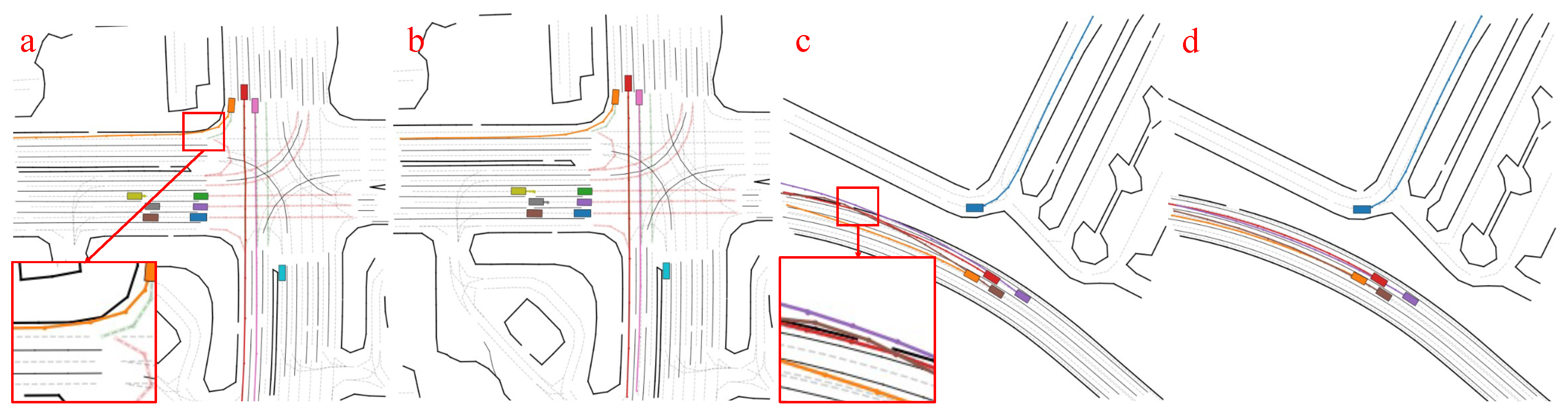
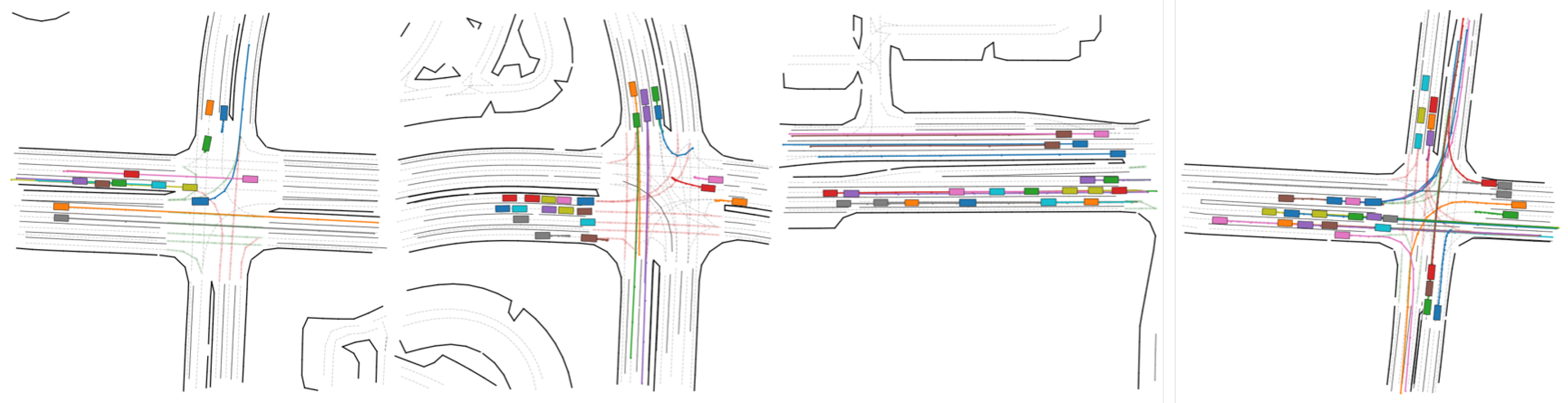
4.3.3. Qualitative Analysis of Trajectory Generation

To intuitively observe the differences between Trafficgen and our model, we visualized the generated trajectories. The visualization results are shown in Figure 3, while Figure 4 demonstrates the model’s performance in generating trajectories across multiple scenarios.

Figure 3 presents a visual comparison of trajectory generation. We set the same initial scenario and used the Trafficgen model and our model, respectively, to generate trajectories in this scenario. Subfigures (a, c) represent traffic flow examples generated by Trafficgen under the same map, while (b, d) show traffic flow generated by our model. As shown in Figure 3, under the same initial conditions, the Trafficgen model fails to incorporate sufficient interagent coordination, resulting in unrealistic lane crossings and unnatural acceleration patterns, as highlighted in subfigure (c). In contrast, our model produces collision-free trajectories with smoother transitions, as observed in subfigure (d).

Figure 4 shows the traffic flow generated by the model under different scenarios, illustrating long-distance trajectories generated based on maps and traffic environments of various scenarios. For better visualization, the trajectories are displayed in static colors. It is worth noting that even with intersections or overlaps, the trajectories show interactive pauses, some of which are caused by traffic lights, while others are due to vehicle avoidance.

4.3.4. Trajectory Prediction Analysis

To fully validate the effectiveness of the model, we degraded it into a trajectory prediction model for further verification. We evaluated our model’s prediction capabilities on the Argoverse Motion Forecasting Dataset. All training and validation scenarios consist of 5-second sequences sampled at 10 Hz, while in the test set, only the first 2 s of trajectories are publicly available. Given the initial 2 s of observation, the Argoverse Motion Forecasting Challenge requires predicting the agent’s future motion for the next 3 s. The final results are shown in

Table 4. Comparison with trajectory prediction models, where the number of predicted trajectories k is set to 6.

Model	minADE↓	minFDE↓	MR↓
LaneGCN[28]	0.87	1.36	0.16
Multipath++ [27]	0.79	1.21	0.13
GANet[29]	0.81	1.16	0.12
HeteroGCN[30]	0.79	1.16	0.12
The proposed	0.75	1.19	0.11

Bold values indicate the best performance.

.

The experimental results show that although the model in this paper is primarily designed for trajectory generation tasks, it performs relatively well in trajectory prediction comparisons, especially in the minADE and MR metrics, demonstrating higher accuracy and success prediction rates. Although it slightly lags behind some models in minFDE, overall, the model in this paper exhibits fairly strong performance.

4.3.5. Ablation Study

We conducted several ablation experiments to evaluate the importance and contribution of each component in the proposed network. These experiments were carried out on the Waymo Motion dataset, with Trafficgen serving as the baseline.

The “Baseline with self-attention” in

Table 5. The test results on the Waymo Motion dataset.

Model	ADE↓	FDE↓
Baseline (Trafficgen)	1.55	4.62
Baseline with self-attention	1.50	4.54
Baseline with cross-attention	1.42	4.58
Baseline with both	1.14	3.67

Bold values indicate the best performance.

demonstrates that the inclusion of self-attention can effectively improve model performance. This mechanism primarily works by helping the model focus on the interactions between vehicles. Specifically, by introducing a multihead self-attention mechanism, the features encoded from the agent are processed, dynamically attending to different parts of the input features, allowing for better capture of the relationship between global and local information, thereby enhancing feature extraction. Experimental results show that this module provides some improvement in FDE, but the improvement in ADE is not significant. This is likely because ADE measures the average deviation of the entire trajectory, while FDE focuses on the final displacement. Therefore, self-attention may primarily benefit the alignment of long-term trajectories.

The “Baseline with cross-attention” in Table 5 demonstrates that the cross-attention mechanism enables an in-depth understanding of global information by capturing the relationship between the map and the vehicles. Specifically, by using a multihead cross-attention mechanism to integrate these two features, the model can capture the complex interactions between map information (such as road structure, traffic signs, etc.) and vehicle states (such as position, speed, etc.). This integration allows the model to more accurately understand the behavior patterns of vehicles in different road environments. Introducing cross-attention significantly enhances ADE performance by integrating static map constraints, while self-attention primarily improves FDE by refining long-term trajectory consistency.

When both self-attention and cross-attention are incorporated, the model performance improves significantly. The self-attention module enhances the interaction features between vehicles, while the cross-attention module compensates for the feature interaction between vehicles and the road, allowing the vehicle to focus more on road information, thereby making the model more realistic and reliable. Additionally, visualizations show that the optimized model performs better, with fewer errors occurring in the trajectory generation across time iterations.

5. Conclusions

In summary, we propose a trajectory generation method based on vehicle–vehicle and vehicle–map interactions. The model incorporates multiple MCG modules for context learning within the scene, introducing self-attention mechanisms for vehicle–vehicle interactions and cross-attention mechanisms for vehicle–map interactions. These mechanisms enable dynamic focus on different parts of the input features, effectively capturing the relationships between global and local information, thus improving feature extraction. Experiments on the Waymo Motion dataset show that compared to our baseline Trafficgen, the proposed method achieves significantly higher accuracy in trajectory generation. It improves the ADE and FDE metrics by 26% and 20%, respectively, from the benchmark values of 1.55 and 4.62. Moreover, ablation studies demonstrate the critical role of the added modules in enhancing performance. Visualization results further indicate that the proposed method improves the plausibility and smoothness of generated trajectories. However, it is important to note that the generated scenes are typical scenarios. Generating risk scenarios is crucial for accelerating autonomous driving simulation testing. Future work will extend this method to adversarial scenario generation, where simulated agents deliberately introduce safety-critical edge cases to further stress-test autonomous driving models.

References

1. Dosovitskiy, A.; Ros, G.; Codevilla, F.; Lopez, A.; Koltun, V. CARLA: An open urban driving simulator. In Proceedings of the Conference on Robot Learning, PMLR, Mountain View, CA, USA, 13–15 November 2017; pp. 1–16. [Google Scholar]
2. Ming, Z.; Jun, L. Smarts: Scalable multi-agent reinforcement learning training school for autonomous driving. arXiv 2020, arXiv:2010.09776. [Google Scholar]
3. Lopez, P.A.; Behrisch, M.; Bieker-Walz, L.; Erdmann, J.; Flötteröd, Y.P.; Hilbrich, R.; Lücken, L.; Rummel, J.; Wagner, P.; Wießner, E. Microscopic traffic simulation using sumo. In Proceedings of the 2018 21st International Conference on Intelligent Transportation Systems (ITSC), IEEE, Maui, HI, USA, 4–7 November 2018; pp. 2575–2582. [Google Scholar] [CrossRef]
4. Waymo LLC. Waymo Open Dataset: An Autonomous Driving Dataset. Available online: https://waymo.com/open (accessed on 26 February 2025).
5. Feng, L.; Li, Q.; Peng, Z.; Tan, S.; Zhou, B. Trafficgen: Learning to generate diverse and realistic traffic scenarios. In Proceedings of the 2023 IEEE International Conference on Robotics and Automation (ICRA), IEEE, London, UK, 29 May–2 June 2023; pp. 3567–3575. [Google Scholar] [CrossRef]
6. Chao, Q.; Bi, H.; Li, W.; Mao, T.; Wang, Z.; Lin, M.C.; Deng, Z. A Survey on Visual Traffic Simulation: Models, Evaluations, and Applications in Autonomous Driving. Comput. Graph. Forum 2020, 39, 287–308. [Google Scholar] [CrossRef]
7. Bergamini, L.; Ye, Y.; Scheel, O.; Chen, L.; Hu, C.; Del Pero, L.; Osiński, B.; Grimmett, H.; Ondruska, P. Simnet: Learning reactive self-driving simulations from real-world observations. In Proceedings of the 2021 IEEE International Conference on Robotics and Automation (ICRA), IEEE, Xi’an, China, 30 May–5 June 2021; pp. 5119–5125. [Google Scholar] [CrossRef]
8. Chang, M.F.; Lambert, J.; Sangkloy, P.; Singh, J.; Bak, S.; Hartnett, A.; Wang, D.; Carr, P.; Lucey, S.; Ramanan, D.; et al. Argoverse: 3d tracking and forecasting with rich maps. In Proceedings of the IEEE/CVF Conference on Computer Vision and Pattern Recognition, Long Beach, CA, USA, 15–20 June 2019; pp. 8748–8757. [Google Scholar]
9. Pérez, J.; Godoy, J.; Villagrá, J.; Onieva, E. Trajectory generator for autonomous vehicles in urban environments. In Proceedings of the 2013 IEEE International Conference on Robotics and Automation, IEEE, Karlsruhe, Germany, 6–10 May 2013; pp. 409–414. [Google Scholar] [CrossRef]
10. Uhrmacher, A.M.; Weyns, D. Multi-Agent Systems: Simulation and Applications; CRC Press: Boca Raton, FL, USA, 2018. [Google Scholar]
11. Gao, Y.; Cao, P.; Yang, A. Realistic Trajectory Generation Using Dynamic Deduction for Stochastic Microscopic Traffic Flow Model; SAE Technical Paper 2024-01-7045; SAE International: Warrendale, PA, USA, 2024. [Google Scholar] [CrossRef]
12. Mullakkal-Babu, F.A.; Wang, M.; van Arem, B.; Shyrokau, B.; Happee, R. A hybrid submicroscopic-microscopic traffic flow simulation framework. IEEE Trans. Intell. Transp. Syst. 2020, 22, 3430–3443. [Google Scholar] [CrossRef]
13. Dobrilko, O.; Bublil, A. Leveraging SUMO for Real-World Traffic Optimization: A Comprehensive Approach. SUMO Conf. Proc. 2024, 5, 179–194. [Google Scholar] [CrossRef]
14. Wheeler, T.A.; Kochenderfer, M.J.; Robbel, P. Initial scene configurations for highway traffic propagation. In Proceedings of the 2015 IEEE 18th International Conference on Intelligent Transportation Systems, IEEE, Gran Canaria, Spain, 15–18 September 2015; pp. 279–284. [Google Scholar]
15. Wheeler, T.A.; Kochenderfer, M.J. Factor graph scene distributions for automotive safety analysis. In Proceedings of the 2016 IEEE 19th International Conference on Intelligent Transportation Systems (ITSC), IEEE, Rio de Janeiro, Brazil, 1–4 November 2016; pp. 1035–1040. [Google Scholar]
16. Jesenski, S.; Stellet, J.E.; Schiegg, F.; Zöllner, J.M. Generation of scenes in intersections for the validation of highly automated driving functions. In Proceedings of the 2019 IEEE Intelligent Vehicles Symposium (IV), IEEE, Paris, France, 9–12 June 2019; pp. 502–509. [Google Scholar]
17. Fang, J.; Zhou, D.; Yan, F.; Zhao, T.; Zhang, F.; Ma, Y.; Wang, L.; Yang, R. Augmented LiDAR simulator for autonomous driving. IEEE Robot. Autom. Lett. 2020, 5, 1931–1938. [Google Scholar] [CrossRef]
18. Caesar, H.; Bankiti, V.; Lang, A.H.; Vora, S.; Liong, V.E.; Xu, Q.; Krishnan, A.; Pan, Y.; Baldan, G.; Beijbom, O. Nuscenes: A multimodal dataset for autonomous driving. In Proceedings of the IEEE/CVF Conference on Computer Vision and Pattern Recognition, Seattle, WA, USA, 13–19 June 2020; pp. 11621–11631. [Google Scholar]
19. Gao, J.; Sun, C.; Zhao, H.; Shen, Y.; Anguelov, D.; Li, C.; Schmid, C. Vectornet: Encoding hd maps and agent dynamics from vectorized representation. In Proceedings of the IEEE/CVF Conference on Computer Vision and Pattern Recognition, Seattle, WA, USA, 13–19 June 2020; pp. 11525–11533. [Google Scholar]
20. Suo, S.; Regalado, S.; Casas, S.; Urtasun, R. Trafficsim: Learning to simulate realistic multi-agent behaviors. In Proceedings of the IEEE/CVF Conference on Computer Vision and Pattern Recognition, Nashville, TN, USA, 20–25 June 2021; pp. 10400–10409. [Google Scholar]
21. Ngiam, J.; Caine, B.; Vasudevan, V.; Zhang, Z.; Chiang, H.T.L.; Ling, J.; Roelofs, R.; Bewley, A.; Liu, C.; Venugopal, A.; et al. Scene transformer: A unified architecture for predicting multiple agent trajectories. arXiv 2021, arXiv:2106.08417. [Google Scholar]
22. Rempe, D.; Philion, J.; Guibas, L.J.; Fidler, S.; Litany, O. Generating useful accident-prone driving scenarios via a learned traffic prior. In Proceedings of the IEEE/CVF Conference on Computer Vision and Pattern Recognition, New Orleans, LA, USA, 18–24 June 2022; pp. 17305–17315. [Google Scholar]
23. Igl, M.; Kim, D.; Kuefler, A.; Mougin, P.; Shah, P.; Shiarlis, K.; Anguelov, D.; Palatucci, M.; White, B.; Whiteson, S. Symphony: Learning realistic and diverse agents for autonomous driving simulation. In Proceedings of the 2022 International Conference on Robotics and Automation (ICRA), IEEE, Philadelphia, PA, USA, 23–27 May 2022; pp. 2445–2451. [Google Scholar]
24. Zhong, Z.; Rempe, D.; Xu, D.; Chen, Y.; Veer, S.; Che, T.; Ray, B.; Pavone, M. Guided conditional diffusion for controllable traffic simulation. In Proceedings of the 2023 IEEE International Conference on Robotics and Automation (ICRA), IEEE, London, UK, 29 May–2 June 2023; pp. 3560–3566. [Google Scholar]
25. Jiang, C.; Cornman, A.; Park, C.; Sapp, B.; Zhou, Y.; Anguelov, D. Motiondiffuser: Controllable multi-agent motion prediction using diffusion. In Proceedings of the IEEE/CVF Conference on Computer Vision and Pattern Recognition, Vancouver, BC, Canada, 17–24 June 2023; pp. 9644–9653. [Google Scholar]
26. Philion, J.; Peng, X.B.; Fidler, S. Trajeglish: Traffic Modeling as Next-Token Prediction. In Proceedings of the Twelfth International Conference on Learning Representations, Vienna, Austria, 7–11 May 2024. [Google Scholar]
27. Varadarajan, B.; Hefny, A.; Srivastava, A.; Refaat, K.S.; Nayakanti, N.; Cornman, A.; Chen, K.; Douillard, B.; Lam, C.P.; Anguelov, D.; et al. Multipath++: Efficient information fusion and trajectory aggregation for behavior prediction. In Proceedings of the 2022 International Conference on Robotics and Automation (ICRA), IEEE, Philadelphia, PA, USA, 23–27 May 2022; pp. 7814–7821. [Google Scholar]
28. Liang, M.; Yang, B.; Hu, R.; Chen, Y.; Liao, R.; Feng, S.; Urtasun, R. Learning lane graph representations for motion forecasting. In Proceedings of the Computer Vision–ECCV 2020: 16th European Conference, Glasgow, UK, 23–28 August 2020; Proceedings, Part II 16. Springer: Berlin/Heidelberg, Germany, 2020; pp. 541–556. [Google Scholar]
29. Wang, M.; Zhu, X.; Yu, C.; Li, W.; Ma, Y.; Jin, R.; Ren, X.; Ren, D.; Wang, M.; Yang, W. Ganet: Goal area network for motion forecasting. In Proceedings of the 2023 IEEE International Conference on Robotics and Automation (ICRA), IEEE, London, UK, 29 May–2 June 2023; pp. 1609–1615. [Google Scholar]
30. Gao, X.; Jia, X.; Li, Y.; Xiong, H. Dynamic scenario representation learning for motion forecasting with heterogeneous graph convolutional recurrent networks. IEEE Robot. Autom. Lett. 2023, 8, 2946–2953. [Google Scholar] [CrossRef]
Figure 1. The main modules of the overall network framework consist of the encoder, decoder, and head. The raw map data and vehicle trajectories are converted into vector information. The encoder is responsible for extracting their respective features and enhancing the interaction features between vehicles, as well as between vehicles and roads. The decoder incorporates anchor point information to generate stable trajectories. Finally, the head leverages the output features from the decoder to produce trajectory information. Here, A represents the number of agents, T represents the time dimension, and each time step uses 7 dimensions to represent the agent’s state. M represents the map vector elements, which have 6 dimensions.
Wevj 16 00145 g001
Figure 2. Vector encoding.
Wevj 16 00145 g002
Figure 3. Visual comparison of trajectory generation. (a,c) represent trajectories generated by Trafficgen, while (b,d) represent trajectories generated by the proposed method. All subfigures are generated under the same initial conditions.
Wevj 16 00145 g003
Figure 4. Model’s ability to generate traffic flows in diverse scenarios.
Wevj 16 00145 g004