Linear Continuous-Time Regression and Dequantizer for Lithium-Ion Battery Cells with Compromised Measurement Quality

Abstract

Battery parameter identification is a key challenge for battery management systems, as parameterizing lithium-ion batteries is resource-intensive. Electrical circuit models (ECMs) provide an alternative, but their parameters change with physical conditions and battery age, necessitating regular parameter identification. This paper presents two modular algorithms to improve data quality and enable fast, robust parameter identification. First, the dequantizer algorithm restores the time series generating the noisy, quantized data using the inverse normal distribution function. Then, the Linear Continuous-Time Regression (LCTR) algorithm extracts exponential parameters from first-order or overdamped second-order systems, deducing ECM parameters and guaranteeing optimality with respect to RMSE. The parameters have low sensitivity to measurement noise since they are continuous-time. Sensitivity analyses confirm the algorithms’ suitability for battery management across various Gaussian measurement noise, accuracy, time constants and state-of-charge (SoC), using evaluation metrics like root-mean-square-error (RMSE) (<2 mV), relative time constant errors, and steady-state error. If the coarseness of rounding is not extreme, the steady-state is restored within a fraction of a millivolt. While a slight overestimation in the lower time constants occurs for overdamped systems, the algorithms outperform the conventional benchmark for first-order systems. Their robustness is further validated in real-life applications, highlighting their potential to enhance commercial battery management systems.

1. Introduction

Battery systems play a crucial role in the shift towards green energy by storing and rapidly transferring electrical energy. While lithium-ion batteries offer high efficiency and performance, their sensitivity to various physical variables and battery chemistry parameters is a challenge. Understanding these nonlinear sensitivities is vital for both performance and safety [1]. Although physics-based bottom-up models can be employed, they are often costly, time-consuming, and energy-intensive for parameter identification [2]. Additionally, the parameters change over time with battery aging, rendering initial identifications less accurate.

The Thévenin equivalent, or equivalent circuit model (ECM), serves as a primary alternative to physics-based models [3] (see Figure 1). It captures input–output battery behavior to the extent the user requires and data quality allows. However, this is an imposed interpretation, hence when the physical variables change, the ECM parameters change with them [4]. Including more variables like state of charge (SoC), temperature, frequency, current, hysteresis state, or pressure results in the curse of dimensionality for parameter lookup tables [5]. This necessitates neglecting certain factors or resorting to online identification of parameters, which requires high-quality measurements of current and terminal voltage as inputs and outputs, respectively.

Parameter identification methods fall into two categories: offline and online algorithms. Offline algorithms process data in batches to find a posterior, while online algorithms incorporate earlier identifications into their prior for updates [6]. This makes the latter computationally more efficient. Identification algorithms can determine either time or frequency domain parameters. They include regression techniques like linear regression, Gaussian processes, support vector machines, neural networks, and ensembles considered as machine learning methods due to their data-driven nature [7]. Input–output methods can identify transfer function, state-space and polynomial model parameters. Such methods produce autoregressive models with exogenous output (ARX, or ARMAX if stochastic). Models can be both linear and nonlinear and are easily computed via online algorithms. For cases where nonlinearities can be separated from the linear model, Hammerstein–Wiener models can be applied [8].

Nonlinear identification methods are notoriously sensitive to initial parameter guesses. Furthermore, they are iterative and time- and memory-intensive. One commonly used linear method, ARX models, becomes particularly sensitive to noise, leading to the overfitting of irrelevant patterns. In order to provide a robust alternative, this paper extends the linear continuous-time regression presented in [9,10] by fitting it to the battery parameter identification problem.

Some challenges that all identification algorithms face are sensitivities to noise, quantization, sampling rate, or the window of the investigated data batch. Assessing lower-cost device feasibility requires understanding the trade-offs in data quality due to sensor limitations. High data quality requires better measurement devices, though this can be impractical or costly. Alternatively, the quality can be improved by software solutions. The issue arises in various fields. In radar applications [11], for example, addressing spectrum corruption from angular quantization during blind phase searches involves low-pass filtering, enhancing phase noise tolerance. Analog-digital conversion [12] tackles sigma-delta quantization error with an optimization algorithm, showing polynomial decay in estimation error with increased sample numbers. Image reconstruction in image processing [13] utilizes generalized expectation maximization for noisy, quantized, and sparse measurements. Seismology [14] finds noise and rounding burden the slope of the Gutenberg–Richter magnitude distribution, revealing biased probability distribution modeling. Compressed sensing studies like [15,16] explore the impact of coarsely quantized, sparse, and noisy data, indicating L1 regularized maximum likelihood’s superiority over L1 regularized least squares. In ARMA or output error (OE) models, parameter bound estimates for quantized data are examined in [17], with such measurements enhancing the innovation signal in [18]. An Unscented Kalman filter is adapted in [19] to handle rounding and Gaussian (normal) measurement noise, noting that high standard deviation (denoted as std. or $\sigma$) has a whitening effect on the combined noise. The Monte Carlo simulation reveals potential sample misplacement due to Gaussian noise in the combined PDF. To achieve parameters with low sensitivity to measurement noise, this approach identifies continuous-time parameters rather than relying on the commonly used linear discrete-time regression.

In our application, the identification of step response functions are studied, where we note two main problems introduced by quantization: (1) the steady-state estimate is biased, (2) the information about the transient is distorted with colored noise. Despite the code’s microcontroller-friendly compactness, an offline algorithm is designed to confirm specific assumptions in the investigated data batch. These assumptions include the following: (1) sufficient charge transfer at the series start for accurate ECM capacitor current estimation, (2) knowledge of SoC at the end of charge transfer due to strong parameter dependency, and (3) a sufficiently long battery cell rest period to capture parameters. The battery cell needs to rest during the identification period since the change in SoC introduces nonlinearities to the investigated time series, and the proposed algorithm assumes constant input. Given the intended accuracy of the application, parameter dependency on current and temperature is neglected.

Contribution. We desire to efficiently determine the ECM parameters of lithium-ion battery cells throughout their lifetime, despite white Gaussian sensor noise and quantization corrupting the terminal voltage measurements. This work proposes two combined, but modular algorithms to address these challenges and investigate their parameter sensitivities. The key contributions (depicted in Figure 1) are as follows:

• A dequantizing algorithm that recovers information lost due to quantization or large noise magnitudes, hence restoring terminal voltage. It utilizes the inverse normal distribution function to reconstruct time series data from quantized measurements corrupted by Gaussian measurement noise.
• The filtered data are processed by the novel Linear Continuous-Time Regression (LCTR) algorithm, capable of deducing gains, time constants, and bias for first-order or overdamped second-order systems.
• Investigation of the combined algorithms’ sensitivity to quantization noise, measurement noise, steady-state, and time constants. Evaluation statistics include root-mean-square-error (RMSE), time-constant errors, and steady-state errors.

The proposed LCTR algorithm aims at providing a fast alternative to nonlinear algorithms, while also ensuring optimality with respect to RMSE. Additionally, we presume that continuous-time parameters have low sensitivity to measurement noise compared to linear regression with discrete-time models.

This paper is structured as follows: Section 2.1 gives an overview of the parameter identification algorithm, then Section 2.2 elaborates on the dequantization and Section 2.3 on the LCTR. The results are described in Section 3 and concluded in Section 4.

2. Methodology

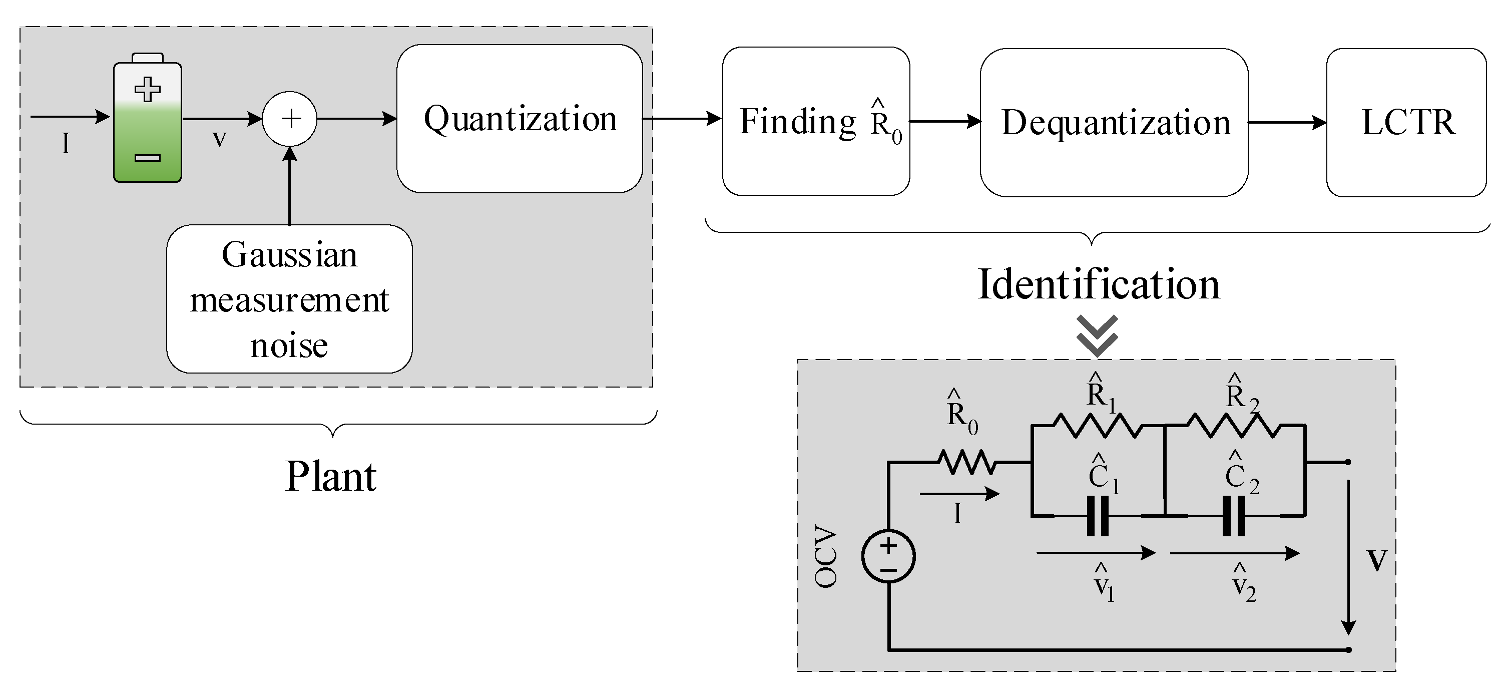
2.1. Overview of the Identification Algorithm

The investigated time series (both simulated and deployed) is 3600 s in length. The battery cell (with $Q=100$ Ah capacity) starts from rest at 85% SoC, is discharged at 30 A from 500 s to 1000 s, and then rests until 3600 s. Time is denoted by t and is a discrete variable when used with an index ☐$\left(t_k\right)$. The sampling time is 1 s. There are five main steps for deducing the parameters of the lithium-ion cell, namely:

I. Finding switching times. Observations indicate that the dynamics behind the $R_0$ step reach steady-state by 1 ms. This means that $R_0$ is overestimated at the 1 s sample period, since after 1 s the voltages over the ECM RC branches are already on the rise. This creates a bias in the estimates of the ECM resistances. To address this, the first sample before a current jump of at least the current threshold 5 A is taken as switching time. There is 1 switch-on and 1 switch-off in each time series.

II. Dequantizing. When applied, the dequantization algorithm operates on the time series data after the switch-off time and estimates the underlying data generating the measurement samples. The first estimate then becomes the first measurement. The last 100 samples are discarded as the receding sample window deteriorates the statistics.

III. Finding $R_0$. The difference between the first sample after switching $v(t_{\mathrm{off}}+1)$ and the mean of 10 samples before switching ${\overline{\mathbf{v}}}_{\mathrm{off}-10:\mathrm{off}}$ is divided by the instantaneous jump in the current I to find $R_0$. The current after switching is zero and is averaged for 500 samples before the jump to reduce the effect of measurement outliers.

$${\widehat{R}}_0={\displaystyle \frac{v(t_{\mathrm{off}}+1\mathrm{s})-{\overline{\mathbf{v}}}_{t_{\mathrm{off}}-10:t_{\mathrm{off}}}}{{\overline{\mathbf{I}}}_{t_{\mathrm{off}}-500:t_{\mathrm{off}}}}},\begin{array}{cc}\hfill {\mathbf{v}}_{t_{\mathrm{off}}-10:t_{\mathrm{off}}}=& {\left[v\left(t_{\mathrm{off}}-10\mathrm{s}\right)\cdots v\left(t_{\mathrm{off}}\right)\right]}^T\hfill \\ \hfill {\mathbf{I}}_{t_{\mathrm{off}}-500:t_{\mathrm{off}}}=& {\left[I\left(t_{\mathrm{off}}-500\mathrm{s}\right)\cdots I\left(t_{\mathrm{off}}\right)\right]}^T\hfill \end{array}$$

(1)

IV. Linear Continuous-Time Regression. The algorithm is used to find the initial values $b_i$ of one or two exponentials, the coefficients $a_i$ of their exponents, and their bias. The index of an exponential is denoted by i. Since the regression has multiple objectives, it is corrupted by colored noise. Hence, the initial values are fixed by stretching them to fit between the first measurement after switching and the mean of the last 100 points of the dequantized time series, i.e.,

$$\begin{array}{cc}\hfill & b_i^{\prime }={\displaystyle \frac{v(t_{\mathrm{off}}+1\mathrm{s})-{\overline{\mathbf{v}}}_{\mathrm{pf},t_{3400}:t_{3500}}}{{\sum }_i{b}_i}},i\in \{1,2\},\hfill \\ & {\overline{\mathbf{v}}}_{\mathrm{pf},t_{3400}:t_{3500}}={\left[v\left(t_{3400}\right)\cdots v\left(t_{3500}\right)\right]}^T.\hfill \end{array}$$

(2)

V. Deducing RC branch parameters. The time constants are the reciprocals of the coefficients of the exponents. The currents through the resistances of the RC branches ${\widehat{i}}_{Ri,t_{\mathrm{off}}}$ are calculated from the differential equation of the RC branch assuming that the exponents are exact and constant before switching off. At last, the RC resistances are obtained from the voltage before switching off and the current through the resistance,

$${\widehat{\tau }}_i={\displaystyle \frac{1}{a_i}},$$

(3)

$${\widehat{R}}_i={\displaystyle \frac{{\widehat{v}}_{i,t_{\mathrm{off}}}}{{\widehat{i}}_{Ri,t_{\mathrm{off}}}}},\mathrm{where}{\widehat{v}}_{i,t_{\mathrm{off}}}=-b_i\mathrm{and}{\widehat{i}}_{Ri,t_{\mathrm{off}}}=\left(1-e^{-(t_{\mathrm{off}}-t_{\mathrm{on}})a_i}\right){\overline{\mathbf{I}}}_{t_{\mathrm{off}}-100:t_{\mathrm{off}}}.$$

(4)

Equations (3) and (4) find the time constants ${\tau }_i$ and the resistances $R_i$ within the Thévenin equivalent in Figure 1, whose parameters are related to the response time and the magnitude of the diffusion voltage, respectively. These parameters will be identified by the LCTR algorithm.

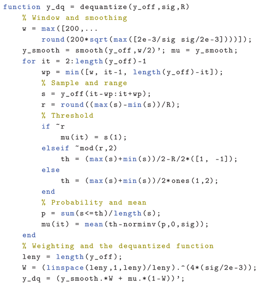
2.2. Dequantizing Algorithm to Alleviate Corrupted Measurements

The dequantizing algorithm aims to recover information lost due to Gaussian measurement noise and quantization. It addresses the rise in the current step response with smoothing and the slower dynamics by leveraging the inverse normal distribution function and the Gaussian assumption. Figure 2a shows how the mean is encoded in the samples. Estimation quality depends on the sampling rate, with limited benefits beyond a level. This sampling rate is typically 1 Hz due to BMS limitations; however, increasing it up to 100 Hz–1 kHz can provide better $R_0$ estimations [20]. The quantization algorithm assumes that a sufficient amount of data is collected for each time instant to estimate the mean, and the electrochemical dynamics are negligible within the investigated time window.

The ratio of samples from the quantization regions uses the inverse normal distribution function to determine the mean value, from which the data are generated. Therefore the data samples and the threshold in the center or right of Figure 2a are utilized to find the distribution on the left. The average estimation error in Figure 2b depends on the location of the mean between the $lR-R/2$ denoted by 0 and $lR$ by 1, where R is the accuracy bit, and $l\in \mathbb{Z}$. The expected value of the error is zero at $lR$. It rises linearly in the vicinity since the number of samples at another value of l is negligible. Close to $lR-R/2$, there are more samples at different l values to describe the distribution. As described in [19], the increasing standard deviation whitens the estimation error. This latter effect is stronger for the green curves with a larger standard deviation.

The estimated mean is calculated at each sampling point based on the sample data batch ${\mathbf{y}}_{\mathrm{s}}\left(t\right)$. The time window w is,

$$\begin{array}{cc}\hfill w=& max\left\{200,⌊200\sqrt{max\left\{{\displaystyle \frac{2\mathrm{mV}}{\sigma }},{\displaystyle \frac{\sigma }{2\mathrm{mV}}}\right\}}⌉\right\}\hfill \\ \hfill {\mathbf{y}}_{\mathrm{s}}\left(t\right)=& {\left[y\left(t_{k-w}\right)\cdots y\left(t_{k+w}\right)\right]}^T,\mathrm{hence}\left|\right|{\mathbf{y}}_{\mathrm{s}}\left(t\right)\left|\right|=2w+1.\hfill \end{array}$$

(5)

The minimum window size is 200 s; it increases proportional to the square of the lack or excess of noise power, since either the estimation error is not whitened sufficiently, or the signal-to-noise-ratio (SNR) is too low. The length of the batch is $\left|\right|{\mathbf{y}}_{\mathrm{s}}\left(t\right)\left|\right|$. The sampling occurs within a symmetric window around the time instant in question, meaning that it is receding at the edges, decreasing both sample length and estimation quality.

The range of the sample $r\left(t\right)$ counted in accuracy bits R is found via Equation (6). Too large an R leads to $r\left(t\right)=0$, hence the quantized data are the sole source of information, giving $\mu \left(t\right)$ as the mean. Nonzero and even / odd $r\left(t\right)$ in Figure 2a depicts the mechanism to find the threshold for the data separation. The thresholds $T_i\left(t\right)$ indicate where data are naturally separated by the rounding (red); otherwise, the estimation becomes biased. In order to alleviate the sampling bias, the inverse normal distribution is evaluated symmetrically from two opposite points of the distribution function.

$$r\left(t\right)={\displaystyle \frac{max{\mathbf{y}}_{\mathrm{s}}\left(t\right)-min{\mathbf{y}}_{\mathrm{s}}\left(t\right)}{R}}$$

(6)

$$\begin{array}{cccc}\hfill & \mathrm{if}r\left(t\right)=0\hfill & \hfill & \mu \left(t\right)={\overline{\mathbf{y}}}_s\left(t\right)\hfill \\ \hfill & \mathrm{if}r\left(t\right)\in {\mathbb{Z}}^{+}\mathrm{is}\mathrm{even}\hfill & \hfill & \left\{\begin{array}{cc}\hfill T_1\left(t\right)=& {\displaystyle \frac{min{\mathbf{y}}_{\mathrm{s}}\left(t\right)+max{\mathbf{y}}_{\mathrm{s}}\left(t\right)}{2}}-{\displaystyle \frac{R}{2}}\hfill \\ \hfill T_2\left(t\right)=& {\displaystyle \frac{min{\mathbf{y}}_{\mathrm{s}}\left(t\right)+max{\mathbf{y}}_{\mathrm{s}}\left(t\right)}{2}}+{\displaystyle \frac{R}{2}}\hfill \end{array}\right.\hfill \\ \hfill & \mathrm{if}r\left(t\right)\in {\mathbb{Z}}^{+}\mathrm{is}\mathrm{odd}\hfill & \hfill & \left\{\begin{array}{cc}\hfill T_1\left(t\right)=& T_2\left(t\right)={\displaystyle \frac{min{\mathbf{y}}_{\mathrm{s}}\left(t\right)+max{\mathbf{y}}_{\mathrm{s}}\left(t\right)}{2}}\hfill \end{array}\right.\hfill \end{array}$$

The sample realization ${\mathbf{y}}_{\mathrm{s}}\left(t\right)$ of the random variable $Y\left(t\right)$ is classified according to how large a proportion of the data points is less than or equal to the threshold $T_i\left(t\right)$. This estimated probability $\widehat{\mathrm{Pr}}\left(Y\left(t\right)\le T_i\left(t\right)\right)$ is expressed in Equation (7). The estimated deviation from the threshold value ${\widehat{\tilde{y}}}_i\left(t\right)$ maximizes the likelihood function $\mathcal{L}{\left(\tilde{y}\left(t\right)|{\mathbf{y}}_{\mathrm{s}}\left(t\right)\right)}_i$.

$$\begin{array}{cc}\hfill \widehat{\mathrm{Pr}}\left(Y\left(t\right)\le T_i\left(t\right)\right)=& {\displaystyle \frac{{\sum }_{j=k-w}^{k+w}q\left(t_j\right)}{\left|\right|{\mathbf{y}}_{\mathrm{s}}\left(t\right)\left|\right|}}i\in \{1,2\},q\left(t_j\right)=\left\{\begin{array}{cc}1\hfill & \mathrm{if}y\left(t_j\right)\le T_i\left(t\right)\hfill \\ 0\hfill & \mathrm{if}y\left(t_j\right)>T_i\left(t\right)\hfill \end{array}\right.\hfill \\ \hfill {\widehat{\tilde{y}}}_i\left(t\right)=& {\mathcal{N}}^{-1}\left(\left.\widehat{\mathrm{Pr}}\left(Y\left(t\right)\le T_i\left(t\right)\right)\right|\mu =0,\sigma \right)\hfill \end{array}$$

(7)

The mean of the sample can then be calculated from the threshold and the deviation as,

$$\begin{array}{cc}\hfill {\widehat{\mu }}_i\left(t\right)=& T_i\left(t\right)-{\widehat{\tilde{y}}}_i\left(t\right)i\in \{1,2\},\hfill \\ \hfill \widehat{\mu }\left(t\right)=& {\displaystyle \frac{{\widehat{\mu }}_1\left(t\right)+{\widehat{\mu }}_2\left(t\right)}{2}},\mathrm{if}r\left(t\right)\in {\mathbb{Z}}^{+}.\hfill \end{array}$$

(8)

At the beginning of the time series, dynamics affect the sample. During this transient region, better results can be obtained if the following smoothing function is used:

$$y_{\mathrm{smooth}}\left(t\right)={\displaystyle \frac{{\sum }_{t_{k-w/4}}^{t_{k+w/4}}y\left(t\right)}{\frac{w}{2}+1}}.$$

(9)

At the edges smoothing is conducted with a receding window, similar to the statistics of the inverse normal distribution. The weighting function $W_{dq}\left(t\right)$ in Equation (10) is used to merge the results of Equations (8) and (9). It consists of a linearly spaced vector with its elements raised to the power c, where c is proportional to the noise power. This enhances noise power to uncover the mean. Finally, the dequantized signal ${\mathbf{y}}_{\mathrm{dq}}$ is obtained from the weighted samples $y_{\mathrm{dq}}\left(t\right)$.

$$\begin{array}{cc}\hfill W_{dq}\left(t\right)=& {\displaystyle \frac{{\left({\left[{\left|\right|\mathbf{y}\left|\right|}_{\mathrm{s}}\left(t\right):-1:1\right]}^T\right)}^c}{{\left|\mathbf{y}\right||}_{\mathrm{s}}\left(t\right)}},\mathrm{where}c=4{\displaystyle \frac{\sigma }{2\mathrm{mV}}},\hfill \\ \hfill y_{\mathrm{dq}}\left(t\right)=& W_{dq}\left(t\right)y_{\mathrm{smooth}}\left(t\right)+\left(1-W_{dq}\left(t\right)\right)\mu \left(t\right).\hfill \end{array}$$

(10)

2.3. Linear Continuous-Time Regression

The challenge with fitting a sum of exponentials to measured data is that it is inherently a nonlinear regression problem. The literature suggests either nonlinear optimization or considers special cases and converts the problem to an approximate linear regression problem to be solved in a closed form. However, most of these methods do not generalize easily to ECM parameter identification. The method below (introduced in [10]) provides a solution to cope with this challenge.

The problem. We desire to take a set of time points $\{t_1,\dots ,t_N\}$ together with a set of data points $\{y_1,\dots ,y_N\}$ and fit them to the model in Equation (11). Parameter m denotes the number of exponential terms in the identification problem. The problem requires that we find the constants $b=\{b_0,b_1,\dots b_m\}$ and $a=\{a_1,a_2,\dots a_m\}$ so as to minimize the root-mean-squared error (RMSE) as defined in Equation (12).

$$\widehat{y}\left(t\right)=b_0+{\displaystyle \sum _{i=1}^m}{b}_i{e}^{-a_{i}t}=b_0+b_1{e}^{-a_{1}t}+b_2{e}^{-a_{2}t}+\cdots$$

(11)

$$\mathrm{RMSE}={\displaystyle \frac{1}{N}}{\displaystyle \sum _{i=1}^N}{\left(y\left(t_i\right)-\widehat{y}\left(t_i\right)\right)}^2.$$

(12)

2.3.1. Single Exponential with and Without Bias

In Equation (13), we begin with the simplest exponential form that also allows a steady-state bias. Its time derivative is calculated in Equation (14). Using Equation (13) and Equation (14), we then find a form without the exponential function explicitly, as stated in Equation (15).

$$\widehat{y}\left(t\right)=b_0+b_1{e}^{-a_{1}t}.$$

(13)

$$\dot{\widehat{y}}\left(t\right)=-b_1{a}_1{e}^{-a_{1}t}.$$

(14)

$$\dot{\widehat{y}}\left(t\right)=-a_1\widehat{y}\left(t\right)+b_0{a}_1.$$

(15)

The initial value of Equation (13) is

$$\widehat{y}\left(0\right)=b_0+b_1.$$

(16)

The next step is to integrate both sides of the expression,

$$\begin{array}{cc}\hfill {\int }_0^t\dot{\widehat{y}}\left(\tau \right)\mathrm{d}\tau & =-a_1{\int }_0^t\widehat{y}\left(\tau \right)\mathrm{d}\tau +{\int }_0^t{b}_0{a}_1\mathrm{d}\tau \hfill \\ \hfill \widehat{y}\left(t\right)& =\left(b_0+b_1\right)+b_0{a}_{1}t-a_1{\int }_0^t\widehat{y}\left(\tau \right)\mathrm{d}\tau .\hfill \end{array}$$

(17)

The rightmost term is approximated in two ways: (i) by replacing $\widehat{y}\left(t\right)$ with the measured data $y\left(t\right)$, and (ii) by replacing the integration with a trapezoidal approximation. We can then write the last line of Equation (17) as Equation (18), where $I_t={\int }_0^{t}t\mathrm{d}t$ is the approximate integral between time 0 and t.

$$\begin{array}{cc}\hfill \widehat{y}\left(t\right)& =\left(b_0+b_1\right)+b_0{a}_{1}t-a_1{I}_t,\mathrm{rewritten}\mathrm{as}\hfill \\ \hfill \widehat{y}\left(t\right)& =A+Bt-C{I}_1\left(t\right).\hfill \end{array}$$

(18)

This form is now linear in the parameters and the values of A, B, and C can be found by standard linear regression,

$$\begin{array}{cc}\hfill \underset{\mathbf{Y}}{\underbrace{\left[\begin{array}{c}{y}_0\\ y_1\\ ⋮\end{array}\right]}}& =\underset{\mathbf{M}}{\underbrace{\left[\begin{array}{ccc}1,& t_0,& -I_1\left(t_0\right)\\ 1,& t_1,& -I_1\left(t_1\right)\\ ⋮& ⋮& ⋮\end{array}\right]}}\underset{\mathbf{X}}{\underbrace{\left[\begin{array}{c}A\\ B\\ C\end{array}\right]}}\hfill \end{array}$$

(19)

The least squares solution is computed as in Equation (20), where † denotes the matrix pseudo-inverse.

$$\mathbf{X}={\mathbf{M}}^{†}\mathbf{Y}$$

(20)

Once we have computed $\mathbf{X}$, and therefore, A, B, and C, we can find the coefficients we desire as,

$$a_1=C,b_0=B/a_1\mathrm{and}{b}_1=A-b_0.$$

(21)

If, for some reason, we happen to be confident that $a_0=0$, then we can simplify the method. We form

$$\begin{array}{cc}\hfill \underset{\mathbf{Y}}{\underbrace{\left[\begin{array}{c}{y}_0\\ y_1\\ ⋮\end{array}\right]}}& =\underset{\mathbf{M}}{\underbrace{\left[\begin{array}{cc}1,& -I_1\left(t_0\right)\\ 1,& -I_1\left(t_1\right)\\ ⋮& ⋮\end{array}\right]}}\underset{\mathbf{X}}{\underbrace{\left[\begin{array}{c}A\\ B\end{array}\right]}}\hfill \end{array}$$

(22)

and compute the least-squares solution $\mathbf{X}={\mathbf{M}}^{†}\mathbf{Y}$. Once we have computed $\mathbf{X}$, and therefore, A, and B, we can find the coefficients we desire as $a_1=B$ and $b_1=A$.

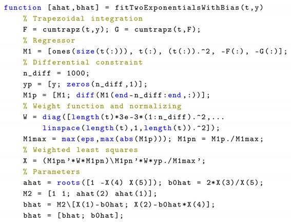
2.3.2. Double Exponential with and Without Bias

The method presented in this work generalizes nicely to higher-order exponential fits. We next consider a double-exponential form with a steady-state bias in Equation (23), with its first and second time derivatives shown in Equation (24). We can express the second-order derivatives from these equations as shown in Equation (25).

$$\widehat{y}\left(t\right)=b_0+b_1{e}^{-a_{1}t}+b_2{e}^{-a_{2}t}.$$

(23)

$$\begin{array}{cc}\hfill \dot{\widehat{y}}& =-b_1{a}_1{e}^{-a_{1}t}-b_2{a}_2{e}^{-a_{2}t}\hfill \\ \hfill \ddot{\widehat{y}}\left(t\right)& =b_1{a}_1^2{e}^{-a_{1}t}+b_2{a}_2^2{e}^{-a_{2}t}.\hfill \end{array}$$

(24)

$$\ddot{\widehat{y}}\left(t\right)=-(a_1+a_2)\dot{\widehat{y}}\left(t\right)-a_1{a}_2\widehat{y}\left(t\right)+b_0{a}_1{a}_2.$$

(25)

The initial values for the model are as follows:

$$\begin{array}{cc}\hfill \widehat{y}\left(0\right)& =b_0+b_1+b_2\hfill \\ \hfill \dot{\widehat{y}}\left(0\right)& =-b_1{a}_1-b_2{a}_2.\hfill \end{array}$$

(26)

Again, we integrate both sides of Equation (25) (we integrate twice here; we will do so one step at a time for clarity),

$$\begin{array}{cc}\hfill {\int }_0^t\ddot{\widehat{y}}\left(\tau \right)\mathrm{d}\tau & =-(a_1+a_2){\int }_0^t\dot{\widehat{y}}\left(\tau \right)\mathrm{d}\tau -a_1{a}_2{\int }_0^t\widehat{y}\left(\tau \right)\mathrm{d}\tau +{\int }_0^t{b}_0{a}_1{a}_2\mathrm{d}\tau \hfill \\ \hfill \dot{\widehat{y}}\left(t\right)-\dot{\widehat{y}}\left(0\right)& =-(a_1+a_2)\left(\widehat{y}\left(t\right)-\widehat{y}\left(0\right)\right)-a_1{a}_2{\int }_0^t\widehat{y}\left(\tau \right)\mathrm{d}\tau +b_0{a}_1{a}_{2}t\hfill \\ \hfill \dot{\widehat{y}}\left(t\right)& =-(a_1+a_2)\widehat{y}\left(t\right)-a_1{a}_2{\int }_0^t\widehat{y}\left(\tau \right)\mathrm{d}\tau +b_0{a}_1{a}_{2}t+\left(b_1{a}_2+b_2{a}_1+b_0(a_1+a_2)\right).\hfill \end{array}$$

(27)

We now integrate again to write,

$$\begin{array}{cc}\hfill {\int }_0^t\dot{\widehat{y}}\left(\tau \right)\mathrm{d}\tau & =-(a_1+a_2){\int }_0^t\widehat{y}\left(\tau \right)\mathrm{d}\tau -a_1{a}_2{\int }_0^t{\int }_0^t\widehat{y}\left(\tau \right)\mathrm{d}\tau \mathrm{d}\zeta +b_0{a}_1{a}_2{\int }_0^t\tau \mathrm{d}\tau \hfill \\ \hfill & +{\int }_0^t\left(b_1{a}_2+b_2{a}_1+b_0(a_1+a_2)\right)\mathrm{d}\tau \hfill \\ \hfill \widehat{y}\left(t\right)& =-(a_1+a_2){\int }_0^t\widehat{y}\left(\tau \right)\mathrm{d}\tau -a_1{a}_2{\int }_0^t{\int }_0^t\widehat{y}\left(\tau \right)\mathrm{d}\tau \mathrm{d}\zeta +b_0{a}_1{a}_2{t}^2/2\hfill \\ \hfill & +\left(b_1{a}_2+b_2{a}_1+b_0(a_1+a_2)\right)t+(b_0+b_1+b_2).\hfill \end{array}$$

(28)

The two integrals are again approximated by replacing $\widehat{y}\left(t\right)$ with the measured data $y\left(t\right)$, and by replacing the integration with a trapezoidal approximation. Then, we can write,

$$\begin{array}{cc}\hfill \widehat{y}\left(t\right)& =-(a_1+a_2)I_1\left(t\right)-a_1{a}_2{I}_2\left(t\right)+b_0{a}_1{a}_2{t}^2/2\hfill \\ \hfill & +\left(b_1{a}_2+b_2{a}_1+b_0(a_1+a_2)\right)t+(b_0+b_1+b_2),\mathrm{rewritten}\mathrm{as}\hfill \\ \hfill \widehat{y}\left(t\right)& =A+Bt+C{t}^2-D{I}_1\left(t\right)-E{I}_2\left(t\right).\hfill \end{array}$$

(29)

As before, this form is now linear in the parameters and the values of A, B, and C can be found via standard linear regression,

$$\begin{array}{cc}\hfill \underset{\mathbf{Y}}{\underbrace{\left[\begin{array}{c}{y}_0\\ y_1\\ ⋮\end{array}\right]}}& =\underset{\mathbf{M}}{\underbrace{\left[\begin{array}{ccccc}1,& t_0,& t_0^2,& -I_1\left(t_0\right),& -I_2\left(t_0\right)\\ 1,& t_1,& t_1^2,& -I_1\left(t_1\right),& -I_2\left(t_1\right)\\ ⋮& ⋮& ⋮& ⋮& ⋮\end{array}\right]}}\underset{\mathbf{X}}{\underbrace{\left[\begin{array}{c}A\\ B\\ C\\ D\\ E\end{array}\right]}}\hfill \end{array}$$

(30)

by computing the least-squares solution $\mathbf{X}={\mathbf{M}}^{†}\mathbf{Y}$. To determine the a and b sets of coefficients from this solution, consider the polynomial $(x-a_1)(x-a_2)=0$. It can be seen that $a_1$ and $a_2$ are roots of the first expression in Equation (31), which can be found using the quadratic equation. We can solve for $b_0$ similarly, using Equation (29). Then, we can assemble a system of equations and solve for $b_1$ and $b_2$ as stated in Equation (32).

$$x^2-Dx+E=0\mathrm{and}{b}_0=2C/E.$$

(31)

$$\left[\begin{array}{c}A-b_0\\ B-b_{0}D\end{array}\right]=\left[\begin{array}{cc}1& 1\\ a_2& a_1\end{array}\right]\left[\begin{array}{c}{b}_1\\ b_2\end{array}\right]$$

(32)

If, for some reason, we happen to be confident that $a_0=0$, then we can simplify the method. We form

$$\begin{array}{cc}\hfill \underset{\mathbf{Y}}{\underbrace{\left[\begin{array}{c}{y}_0\\ y_1\\ ⋮\end{array}\right]}}& =\underset{\mathbf{M}}{\underbrace{\left[\begin{array}{cccc}1,& t_0,& -I_1\left(t_0\right),& -I_2\left(t_0\right)\\ 1,& t_1,& -I_1\left(t_1\right),& -I_2\left(t_1\right)\\ ⋮& ⋮& ⋮& ⋮\end{array}\right]}}\underset{\mathbf{X}}{\underbrace{\left[\begin{array}{c}A\\ B\\ C\\ D\end{array}\right]}}\hfill \end{array}$$

(33)

and compute the least-squares solution $\mathbf{X}={\mathbf{M}}^{†}\mathbf{Y}$. Once we have computed $\mathbf{X}$ we can then solve for $a_1$ and $a_2$ as roots of the polynomial $x^2-Cx+D=0$, which can be found using the quadratic equation. Then, we solve the system of equations Equation (34) to find $b_1$ and $b_2$.

$$\left[\begin{array}{c}A\\ B\end{array}\right]=\left[\begin{array}{cc}1& 1\\ a_2& a_1\end{array}\right]\left[\begin{array}{c}{b}_1\\ b_2\end{array}\right]$$

(34)

2.3.3. The LCTR Algorithm

Special modifications were made to improve LCTR performance. The modified outputs are noted by apostrophe.

Weighted least squares and normalization. The least square solution of Equation (20) is modified to the weighted least squares solution (for both orders) in Equation (35). Normalization was applied to improve matrix conditioning; here $max|{\mathbf{M}}_{:j}|$ denotes the maximum absolute value of column j. The vector $\mathbf{X}$ consists of the matrix columns $X_j$.

$$X_j={\displaystyle \frac{{\left({\mathbf{M}}^{\prime T}\mathbf{W}{\mathbf{M}}^{\prime }\right)}^{-1}{\mathbf{M}}^{\prime }\mathbf{W}\mathbf{y}}{max|{\mathbf{M}}_{:j}|}},\mathrm{where}{\mathbf{M}}_{ij}^{\prime }={\displaystyle \frac{{\mathbf{M}}_{ij}}{max|{\mathbf{M}}_{:j}|}}\forall \{i,j\}$$

(35)

Differential constraint for the second-order case. Reduced data quality can often lead to one of the time constants being incorrectly identified as negative. In order to enforce stable parameters, differential constraints were introduced in Equation (36) for the last 1000 data points, equating the differential of the estimated output with zero. Note that $\mathbf{X}$ is constant, hence $\dot{\mathbf{X}}=\mathbf{0}$. The augmented matrices are ${\mathbf{M}}^{\prime }$ and ${\mathbf{Y}}^{\prime }$. The weight function for the differential constraint $\mathbf{W}$ in Figure 3 increases in a quadratic manner after the sample point 2500, since subsequent data points are expected to change their values less than the ones prior.

$$\begin{array}{cc}\hfill \mathbf{Y}=& \mathbf{M}\mathbf{X},\hfill \\ \hfill {\dot{\mathbf{Y}}}_{t_{2600}:t_{3600}}=\mathbf{0}=& {\dot{\mathbf{M}}}_{t_{2600}:t_{3600},:}\mathbf{X},\hfill \\ & \mathrm{where}\left\{\begin{array}{cc}\hfill {\mathbf{Y}}_{t_{2600}:t_{3600}}=& {\left[Y\left(t_{2600}\right)\cdots Y\left(t_{3600}\right)\right]}^T,\hfill \\ \hfill {\mathbf{M}}_{t_{2600}:t_{3600},:}=& {\left[\mathbf{M}\left(t_{2600},i\right)\cdots \mathbf{M}\left(t_{3600},i\right)\right]}^T\forall i,\hfill \end{array}\right.\hfill \\ & {\mathbf{Y}}^{\prime }=\left[\begin{array}{c}\hfill \mathbf{Y}\\ \hfill \mathbf{0}\end{array}\right],{\mathbf{M}}^{\prime }=\left[\begin{array}{c}\hfill \mathbf{M}\\ \hfill \dot{\mathbf{M}}\end{array}\right].\hfill \end{array}$$

(36)

Transient weighting. Figure 3 also shows that weighting on data points at the rise times of the transients is greater than that at the end of the data series. This ensures that the more informative dynamics at the beginning dominate the fitting so that the right time constants are found. Due to the nature of least squares, the longer the data series, the less exact the rise periods are fitted. Furthermore, since regression techniques assume white noise [7], the noise coloring due to using larger time windows (see Equation (5)) reduces estimation quality. This was taken into consideration when choosing window sizes.

2.4. Matlab Implementations

• The Matlab code of the dequantizer:

• The Matlab code for second-order fit:

3. Results

3.1. Sensitivity Analysis Overview

A sensitivity analysis was performed to assess the performance and robustness of the algorithms with respect to Gaussian measurement noise $\sigma$, resolution R, state of charge (SoC, analogous to open-circuit voltage), and time constants ${\tau }_i$. Evaluation metrics included RMSE (see Equation (12)), relative time constant errors (${\tilde{\tau }}_i/{\tau }_i$, where $\tilde{\phantom{a}}$ denotes estimation error), and steady-state errors. Steady-state errors are approximated as the error at the last time instant of the window. 

Table 1. Nominal, extreme values and number of parameter test points for second order systems (Figure 1). The test points are distributed logarithmically, except for SoC, which is linear. The base of the logarithm is 2 for $\sigma$ and R and 1.5 for ${\tau }_1$ and ${\tau }_2$.

	$\mathit{\sigma }$	R	${\mathit{\tau }}_1$	${\mathit{\tau }}_2$	${\mathit{R}}_0$	${\mathit{R}}_1$	${\mathit{R}}_2$	$\mathit{SoC}\left({\mathit{t}}_0\right)$
Nominal value	2 mV	0.31 mV	22 s	647 s	0.63 m$\Omega$	0.47 m$\Omega$	0.24 m$\Omega$	80%
Minimum value	0.25 mV	0.63 mV	4.3 s	128 s	-	-	-	10%
Maximum value	16 mV	10 mV	111 s	3275 s	-	-	-	100%
Number of test points	7	6	9	9	1	1	1	91

displays nominal and extreme parameter values. Nominal values are used when not distributed.

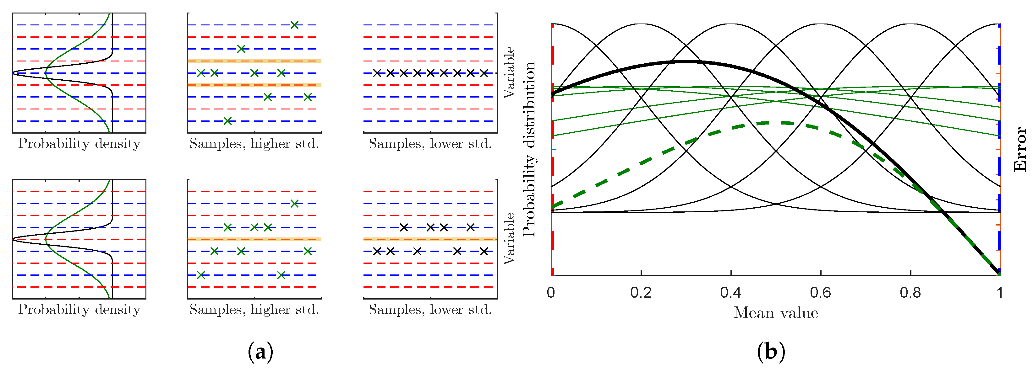
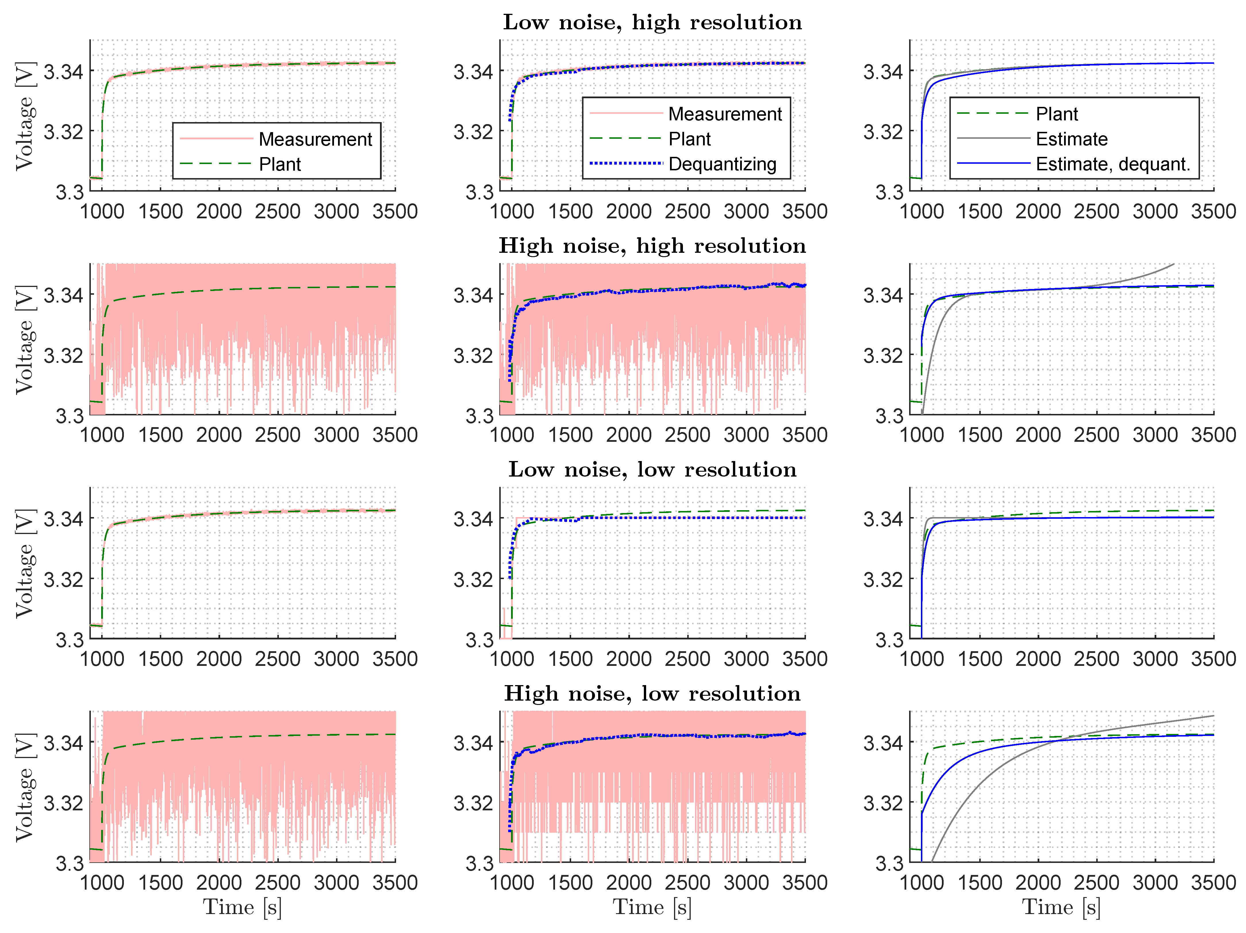
3.2. Visualization of Parameter Identification

First, visualizations of the dequantizing and the LCTR time series are shown for minimal and maximal resolution and Gaussian noise, using a second-order model. Next, RMSE improvement with the dequantizer is shown; the dequantizer is used hereafter in what follows. Then, relative time constant error sensitivity to time constants is shown in order to explore how the combined locations of the two time constants challenge the program. Tests on the first-order system show that a reduced number of parameters are easier to find. A comparison of RMSE improvement and relative time constant errors with those of a benchmark algorithm follows. Steady-state errors are plotted against accuracy and state-of-charge to highlight biased estimation due to coarse rounding. Finally, a real-life scenario test is presented. Matlab experiments show that the dequantizier takes 20 ms, and the LCTR takes 40 ms for second-order and 20 ms for first-order systems.

Figure 4 shows the performance of the LCTR for low/high values of Gaussian noise and resolution. The first row shows that the dequantizer’s smoothing effect slightly distorts the data; by using overlapping sample batches, it adds a correlation between data points. However, as soon as the data quality decreases and the data statistics begin to convey more than the individual points, it becomes useful. When the data are coarsely quantized, the steady-state is missed by the estimation. The LCTR estimates unstable time constants for the dataset with high Gaussian noise without dequantization. It also overestimates low time constants for large Gaussian noise standard deviation.

Figure 5 displays RMSE variations based on accuracy and Gaussian noise standard deviation, comparing unfiltered and dequantized cases. The red regions on the right indicate challenges posed by the Gaussian noise, particularly evident at a low resolution, but notably mitigated by dequantization. Yet, at low Gaussian noise, dequantization’s impact on RMSE is not substantial due to the coloring effect of quantization, where the dequantizer lacks sufficient information to recover the steady-state. Given the improvements, subsequent usage of the dequantizer is implied.

Figure 6 depicts relative time constant errors $(\widehat{{\tau }_i}-{\tau }_i)/{\tau }_i$ for varying time constant values. The estimation of ${\tau }_1$ deteriorates with lower values since limited samples are used to describe the rise. It also worsens when ${\tau }_2$ is lower or ${\tau }_1$ is higher, indicating challenges when the two time constants are close together, which leads the LCTR to mix information about the exponentials. The relative error of ${\tau }_2$ increases with larger values, likely due to the incomplete convergence captured in the 2500 s time window.

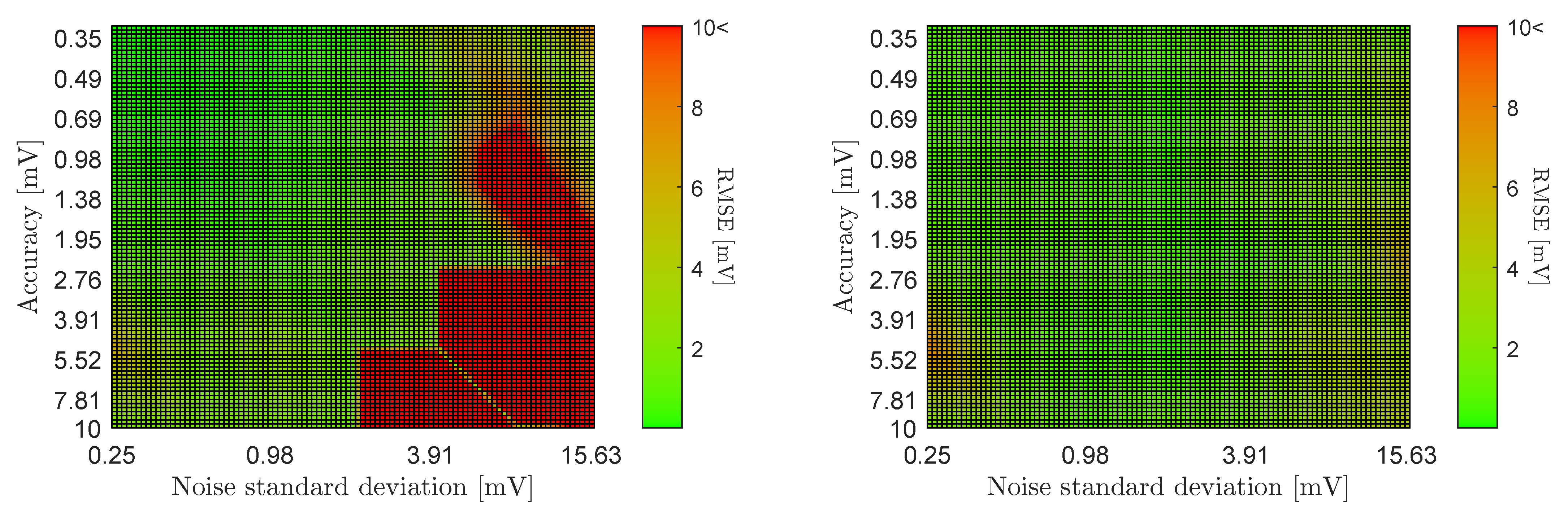
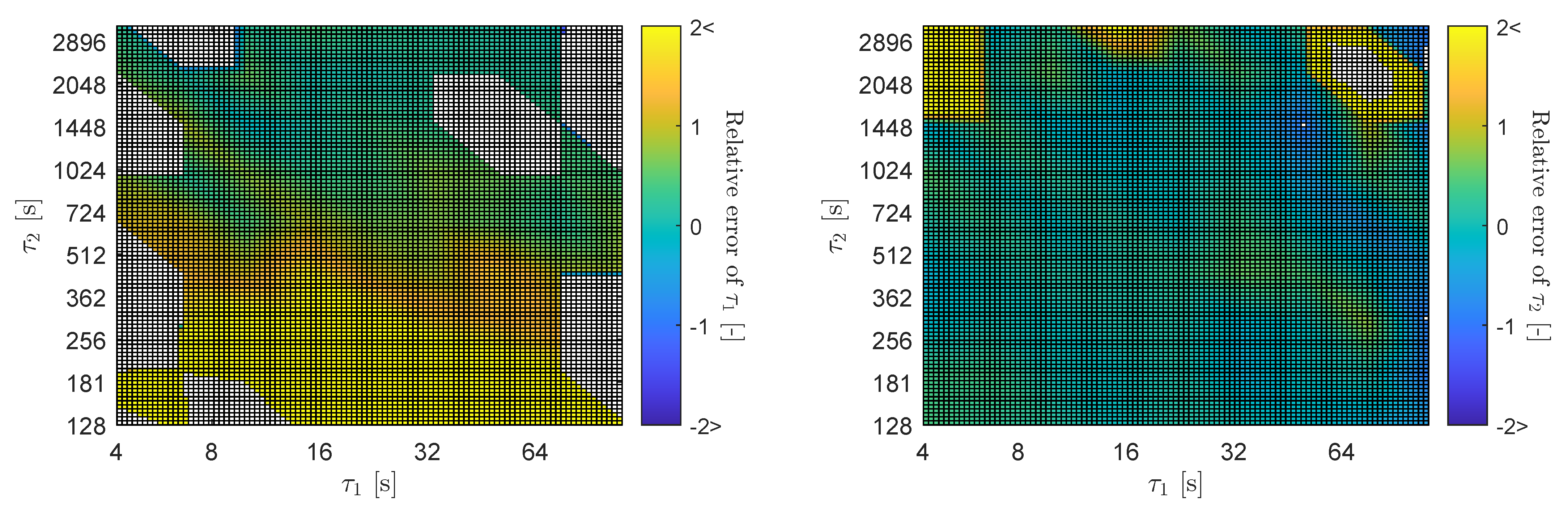
3.3. Parameter Sensitivities for the First-Order Model

The benchmark algorithm refers to the analytical method used to find the parameters of a first-order model. If the sampling rate is high enough, the data are deterministic, and the end of the time series is near the steady-state, then it gives nearly exact estimations. The mean of the last 100 samples is taken as the estimated steady-state. The estimated initial value is the difference between the initial data point and the steady-state. The time constant is the time when the $1-e^{-t/\tau }=1-e^{-1}=63\%$ of the initial value is attained by the curve. This algorithm takes 7 ms.

Tests on the first-order model assumed the geometric mean of ${\tau }_1$ and ${\tau }_2$, i.e., 119.2 s, as the time constant. Figure 7 left shows the LCTR RMSE improvement compared to the benchmark for first-order systems. It is larger in regions with a high Gaussian noise standard deviation due to the inherent robustness of the LCTR. However, it worsens in the coarsely rounded region with low noise. Figure 7 right shows the steady-state error of the LCTR plotted against accuracy and SoC (similar results for the benchmark). The OCV is a strictly monotonic function of the SoC, and it equates to the steady-state; hence the rounding error shows periodicity over SoC as displayed in Figure 2b. The dequantizer reduces the steady-state error to a fraction of a mV in most of the region, except where the data are coarsely rounded.

3.4. Field Test Results

Figure 8 shows one of a series of measurements that were made to test a LiFePO₄ cell [21]. The battery cell was charged for 15 min then rested for 40 min with data captured at 10 mV accuracy. The dequantizer algorithm restored the data sufficiently for the LCTR to process it. In doing so, the LCTR found $R_0=0.9\mathrm{m}\Omega$, $R_1=1.1\mathrm{m}\Omega$, $R_2=1.5\mathrm{m}\Omega$, ${\tau }_1=225$ s and ${\tau }_2=859$ s for this particular cell. Based on the data and general experience with LiFePO₄ chemistry (see such a cell from another manufacturer in [2]), all the parameters are realistic, except for ${\tau }_1$, which is normally expected to be around one minute.

4. Conclusions

This work addresses the parameter estimation of single and double exponential functions with application to lithium-ion battery cells, under compromised data quality conditions. Its main contributions are as follows: (i) the dequantizer algorithm, (ii) Liner Continuous-Time Regression (LCTR), and (iii) corresponding sensitivity analysis. The dequantizer is able to recover the shape of the underlying data in the presence of Gaussian noise, although it introduces some correlation due to overlapping sample windows and fails to find the steady-state at extremely coarse resolution. The LCTR demonstrates robustness after data processing by the dequantizer and outperforms an analytical benchmark algorithm, which is a typical commercial application. The RMSE is normally below 2 mV and the steady-state error is within a fraction of a millivolt if rounding is not extremely coarse. The lower time constant of second-order systems may be overestimated under higher noise levels. In summary, the algorithm is fast, robust and analytically sound to estimate the battery parameters throughout their lifespan.

There are several avenues of improvement for future work. The dequantizer used a maximum of two thresholds. Dividing the data along all possible thresholds can further improve recovery. The author observed that higher sampling rates improve the lower time constant’s estimate, warranting a sensitivity analysis. Addressing missing or intermittent data could also be included in such an analysis. Lastly, converting the least squares algorithm to a recursive formulation could potentially reduce memory usage and improve algorithm speed.

References

1. Pinter, Z.M.; Papageorgiou, D.; Rohde, G.; Marinelli, M.; Træholt, C. Review of control algorithms for reconfigurable battery systems with an industrial example. In Proceedings of the 2021 56th International Universities Power Engineering Conference (UPEC), Middlesbrough, UK, 31 August–3 September 2021; pp. 1–6. [Google Scholar]
2. Pinter, Z.M.; Engelhardt, J.; Rohde, G.; Træholt, C.; Marinelli, M. Validation of a Single-Cell Reference Model for the Control of a Reconfigurable Battery System. In Proceedings of the 2022 International Conference on Renewable Energies and Smart Technologies (REST), Tirana, Albania, 28–29 July 2022; Volume 1, pp. 1–5. [Google Scholar]
3. Plett, G.L. Battery Management Systems, Volume II: Equivalent-Circuit Methods; Artech House: Norwood, MA, USA, 2015. [Google Scholar]
4. Marinelli, M.; Calearo, L.; Engelhardt, J.; Rohde, G. Electrical Thermal and Degradation Measurements of the LEAF e-plus 62-kWh Battery Pack. In Proceedings of the 2022 International Conference on Renewable Energies and Smart Technologies (REST), Tirana, Albania, 28–29 July 2022; Volume 1, pp. 1–5. [Google Scholar]
5. Pinter, Z.M.; Rohde, G.; Marinelli, M. Comparative Analysis of Rule-Based and Model Predictive Control Algorithms in Reconfigurable Battery Systems for EV Fast-Charging Stations. J. Energy Storage. 2023. Available online: https://papers.ssrn.com/sol3/papers.cfm?abstract_id=4882648 (accessed on 2 July 2024).
6. Åström, K.J.; Wittenmark, B. Adaptive Control; Courier Corporation: Chelmsford, MA, USA, 2008. [Google Scholar]
7. Bishop, C. Pattern Recognition and Machine Learning; Springer: Berlin/Heidelberg, Germany, 2006; Volume 2, pp. 531–537. [Google Scholar]
8. Wills, A.; Schön, T.B.; Ljung, L.; Ninness, B. Identification of hammerstein—Wiener models. Automatica 2013, 49, 70–81. [Google Scholar] [CrossRef]
9. Foss, S.D. A method of exponential curve fitting by numerical integration. Biometrics 1970, 26, 815–821. [Google Scholar] [CrossRef]
10. Plett, G.L. A Linear Method to Fit Equivalent Circuit Model Parameter Values to HPPC Relaxation Data From Lithium-Ion Cells. ASME Lett. Dyn. Syst. Control 2025, 5, 011003. [Google Scholar] [CrossRef]
11. Rodrigo Navarro, J.; Kakkar, A.; Schatz, R.; Pang, X.; Ozolins, O.; Udalcovs, A.; Popov, S.; Jacobsen, G. Blind phase search with angular quantization noise mitigation for efficient carrier phase recovery. Photonics 2017, 4, 37. [Google Scholar] [CrossRef]
12. Saab, R.; Wang, R.; Yılmaz, Ö. Quantization of compressive samples with stable and robust recovery. Appl. Comput. Harmon. Anal. 2018, 44, 123–143. [Google Scholar] [CrossRef]
13. Qiu, K.; Dogandzic, A. Sparse signal reconstruction from quantized noisy measurements via GEM hard thresholding. IEEE Trans. Signal Process. 2012, 60, 2628–2634. [Google Scholar] [CrossRef]
14. Márquez-Ramírez, V.; Nava, F.; Zúñiga, F. Correcting the Gutenberg–Richter b-value for effects of rounding and noise. Earthq. Sci. 2015, 28, 129–134. [Google Scholar] [CrossRef]
15. Stanković, I.; Brajović, M.; Daković, M.; Ioana, C.; Stanković, L. Quantization in compressive sensing: A signal processing approach. IEEE Access 2020, 8, 50611–50625. [Google Scholar] [CrossRef]
16. Zymnis, A.; Boyd, S.; Candes, E. Compressed sensing with quantized measurements. IEEE Signal Process. Lett. 2009, 17, 149–152. [Google Scholar] [CrossRef]
17. Casini, M.; Garulli, A.; Vicino, A. Bounding nonconvex feasible sets in set membership identification: OE and ARX models with quantized information. IFAC Proc. Vol. 2012, 45, 1191–1196. [Google Scholar] [CrossRef]
18. Yu, C.; You, K.; Xie, L. Quantized identification of ARMA systems with colored measurement noise. Automatica 2016, 66, 101–108. [Google Scholar] [CrossRef]
19. Xu, J.; Li, J.; Xu, S. Analysis of quantization noise and state estimation with quantized measurements. J. Control Theory Appl. 2011, 9, 66–75. [Google Scholar] [CrossRef]
20. Steinstraeter, M.; Gandlgruber, J.; Everken, J.; Lienkamp, M. Influence of pulse width modulated auxiliary consumers on battery aging in electric vehicles. J. Energy Storage 2022, 48, 104009. [Google Scholar] [CrossRef]
21. GWL/Power CALB CA100FI—Lithium Cell LiFePO4 (3.2 V/100 Ah), Datasheet. Available online: https://files.gwl.eu/ (accessed on 1 January 2024).
Figure 1. (Top): Data generation (meaning the assumptions for the identification and the simulation), and ECM parameter identification. (Bottom): the Thévenin equivalent (or ECM, see [2]) of a second-order model. Estimation is denoted by ^ , where ☐ is the variable of interest. Open circuit voltage (OCV) is found from a lookup table based on the SoC. The SoC is calculated by Coulomb-counting Δ S o C = 100 % Q I d t , where Q is capacity and I is current.
Wevj 16 00116 g001
Figure 2. Features of the dequantizing algorithm. (a) Choosing threshold (orange) for the inverse normal distribution. Rounded values are dashed blue. (top): odd number of values, (bottom): even number of values. (Left): Gaussian distribution, (center): large std. (green), (right): low std. (black). (b) Estimation error dependence on the mean’s position between the rounded value (1) and the average of neighboring rounded values (0). Green: large std. Black: low std.
Wevj 16 00116 g002
Figure 3. The LCTR weighting function. The first 2500 samples set a preference to model early data points, the last 1000 samples weight the steady-state differential.
Wevj 16 00116 g003
Figure 4. Dependency of estimation quality on Gaussian noise and resolution for an overdamped second-order system.
Wevj 16 00116 g004
Figure 5. RMSE for the unfiltered (left) and the dequantized (right) estimation for an overdamped second-order system.
Wevj 16 00116 g005
Figure 6. Relative error of τ 1 (left) and τ 2 (right). White areas denote estimations below 10% or above 10 times of the true value.
Wevj 16 00116 g006
Figure 7. (left) Difference in RMSE in mV for benchmark and the LCTR. Yellow means larger error for the benchmark, dark blue means larger error for the LCTR. The investigated system is a first-order system. (right) Steady-state error in mV depicted for LCTR (similar results found for the benchmark).
Wevj 16 00116 g007
Figure 8. Results of the first-order algorithm on a field test with a lithium-ion phosphate cell. (top) current time series, (bottom) measurement, dequantized and estimated voltage time series. The spikes in the voltage occur because the model uses the noisy current measurement as an input.
Wevj 16 00116 g008