Research on Decoupling Control of Four-Wheel Steering Distributed Drive Electric Vehicles

Abstract

To address the issue of limited accuracy in vehicle lateral and longitudinal dynamics control—caused by the strong coupling and nonlinearity between the four-wheel steering and distributed drive systems, particularly under crosswind disturbances—a control method integrating differential geometric decoupling with robust control is proposed. This integrated approach mitigates coupling effects among the vehicle motions in various directions, thereby enhancing overall robustness. The control architecture adopts a hierarchical structure: the upper layer takes the deviation between the ideal and actual models as input and generates longitudinal, yaw, and lateral control laws via robust control; the middle layer employs differential geometric methods to decouple the nonlinear system, deriving the total driver-required driving torque, additional yaw moment, and rear-wheel steering angle; and the lower layer utilizes a quadratic programming algorithm to optimize the distribution of driving torque across the four wheels. Finally, simulation verification is conducted based on a co-simulation platform using TruckSim 2022 and MATLAB R2024a/Simulink. The simulation results demonstrate that, compared to the sliding mode control (SMC) and the uncontrolled scenario, the proposed method improves the driving stability and safety of the four-wheel steering distributed drive vehicle under multiple operating conditions.

1. Introduction

With the rapid advancement of intelligent vehicle technologies, modern chassis control systems are evolving toward integration, electrification, and intelligence. In recent years, integrated chassis control has emerged as a critical research focus in the dynamics of distributed drive electric vehicles (DDEVs) [1,2]. DDEVs, characterized by precise handling, short transmission chains, low energy losses, and compact structures, provide an optimal hardware platform for vehicle stability control via direct yaw moment control (DYC) [3,4,5]. As a critical safety control method, four-wheel steering (4WS) technology actively intervenes in vehicle steering to approximate ideal response characteristics, thereby significantly enhancing handling stability [6,7]. Currently, numerous researchers are conducting extensive investigations into the integrated control of 4WS and distributed drive systems.

Zuo et al. [8] proposed a hierarchical control strategy. The upper-layer controller employed sliding mode control to coordinate the rear-wheel steering angle and direct yaw moment, while the lower-layer controller optimized torque distribution based on the tire load rate to enhance vehicle stability. Chen et al. [9] developed a hierarchical coordinated controller integrating active front steering (AFS) and DYC using extension coordination control theory, with wheel torque allocation optimized through quadratic programming. Zakaria et al. [10] implemented fuzzy logic-based DYC for an eight-wheel independently driven vehicle. Jin et al. [11] combined fuzzy control with a linear quadratic regulator (LQR) for 4WS implementation, activating additional yaw moment when exceeding predefined thresholds. While these approaches effectively improve vehicle stability, they generally neglect longitudinal dynamics analysis.

Lin et al. [12] implemented independent control of longitudinal, lateral, and yaw motions using a backstepping sliding mode approach, significantly enhancing vehicle lateral stability. Ni et al. [13] developed separate longitudinal and robust lateral controllers for autonomous racing vehicles, demonstrating the practical applicability of the algorithm. While these decentralized control architectures feature relatively simple algorithms and modest hardware requirements, they insufficiently address the inherent coupling between vehicle longitudinal and lateral dynamics.

This oversight presents two major challenges: First, both speed control and stability control in DDEVs are achieved through wheel torque regulation, creating strong subsystem coupling due to conflicting control objectives. Second, tire force variations during steering operations further intensify longitudinal–lateral coupling, significantly complicating precise vehicle dynamics control. Given the strongly coupled and nonlinear nature of vehicle dynamics systems, researchers have extensively investigated various decoupling methodologies.

Yu et al. [14] developed a feedback–feedforward neural network decoupling strategy that achieved long-range decoupled tracking and improved tracking accuracy under emergency longitudinal-lateral coupled conditions. Zhang et al. [15] implemented an extreme learning machine (ELM)-based neural network inverse dynamics system, successfully decoupling the longitudinal, lateral, yaw, and roll motions in chassis-integrated control. This algorithm demonstrated excellent path-tracking performance when applied to autonomous vehicles. Chang et al. [16] introduced a novel CNN-LSTM inverse system design methodology that effectively decoupled lateral and yaw dynamics while enhancing both tracking capability and stability. Liang et al. [17] employed neural networks to establish a pseudo-linear system and applied internal model control theory to coordinate longitudinal and lateral motion control, obtaining satisfactory control performance. Although these neural network-based inverse system approaches exhibit favorable decoupling performance and accuracy, their heavy dependence on extensive offline training data results in compromised real-time processing capability and limited emergency handling performance.

Differential geometry and differential flatness theory represent prevalent mathematical approaches for addressing nonlinear control problems, offering significant computational complexity reduction. Wang et al. [18] successfully decoupled vehicle roll and planar dynamics using differential geometry methods, incorporating a load transfer ratio-based control trigger that effectively regulated roll angle and yaw rate independently. Wu et al. [19] conducted comprehensive analysis of chassis system coupling relationships, establishing a pseudo-linear system through inverse system serialization to achieve decoupled control of lateral, yaw, and roll motions. However, these approaches uniformly neglected the influence of longitudinal motion on lateral dynamics. Wang et al. [20] demonstrated the differential flatness property in three-degree-of-freedom (3-DOF) vehicle models and implemented a backstepping controller for longitudinal-lateral decoupled control. Nevertheless, the experimental validation omitted external disturbance testing, leaving the disturbance rejection capability of the system unverified. Gao et al. [21] applied differential geometry theory to decouple longitudinal-lateral vehicle dynamics, developing a virtual control law with tire cornering stiffness estimation that enhanced intelligent vehicle path-tracking. However, this method exhibited insufficient precision in yaw rate control.

While the aforementioned studies have all employed differential geometric methods, they primarily focus on front-wheel-steering electric vehicles, rather than distributed drive electric vehicles capable of four-wheel steering. Based on this, this paper proposes a hierarchical controller that integrates differential geometric decoupling control with robust control. The controller decouples the three-input-three-output nonlinear vehicle system into three independent subsystems, enabling separate control of longitudinal, yaw, and lateral motions while enhancing disturbance rejection capabilities. Validation was conducted through TruckSim-MATLAB/Simulink co-simulation under various operating conditions. Compared to sliding mode control (SMC) and uncontrolled scenarios, the proposed method demonstrates superior performance, maintaining precise longitudinal velocity tracking while significantly improving yaw stability.

2. Vehicle Dynamics Modeling

2.1. Nonlinear 3-DOF Dynamic Model of 4WS Vehicle

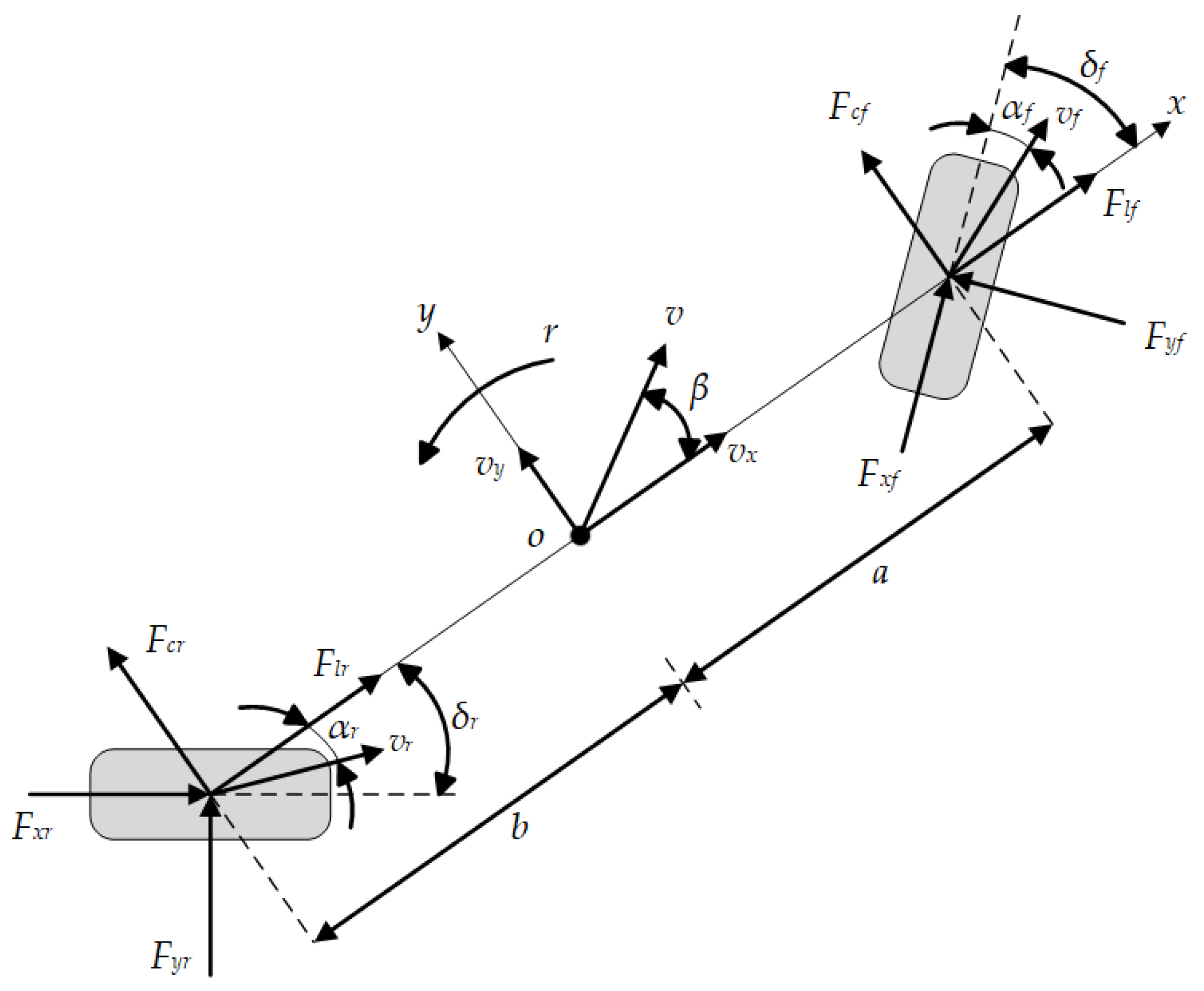
The vehicle is simplified as a single-track model with the following assumptions: tire rolling resistance is negligible; load transfer between the front and rear axles is disregarded; and suspension system effects are excluded. The model considers only the longitudinal, lateral, and yaw dynamics of a 4WS vehicle. As shown in Figure 1, the system inputs are directly defined as the front/rear wheel steering angles and tire forces. Based on Newton’s second law, the 3-DOF vehicle dynamics equations are derived as follows:

$$\left\{\begin{array}{l}m{\dot{v}}_x=m{v}_{y}r+F_{lf}+F_{lr}+\Delta F_{wx}\\ m{\dot{v}}_y=-m{v}_{x}r+F_{cf}+F_{cr}+\Delta F_{wy}\\ I_z\dot{r}=a{F}_{cf}-b{F}_{cr}+\Delta M_{wz}\end{array}\right.$$

(1)

In the formula, $m$ denotes the total vehicle mass; $r$ is the yaw rate of the vehicle; $v_x$ and $v_y$ are the longitudinal velocity and lateral velocity at the center of mass of the vehicle, respectively; $F_{lf}$ and $F_{lr}$ are the components of the longitudinal and lateral forces on the front and rear axles along the x-axis, respectively; and $F_{cf}$ and $F_{cr}$ are the components of the longitudinal and lateral forces on the front and rear axles along the y-axis, as determined by Equation (2). $I_z$ is the moment of inertia of the vehicle body and $a$ and $b$ are the longitudinal distances from the vehicle center of mass to the front and rear axles, respectively. $\Delta F_{wx}$, $\Delta F_{wy}$, and $\Delta M_{wz}$ are the longitudinal drag force, lateral drag force, and yaw resistance moment generated by crosswind, respectively, acting as external disturbances during vehicle travel.

$$\left\{\begin{array}{l}{F}_{lf}=F_{xf}\cos {\delta }_f-F_{yf}\sin {\delta }_f\\ F_{lr}=F_{xr}\cos {\delta }_r+F_{yr}\sin {\delta }_r\\ F_{cf}=F_{xf}\sin {\delta }_f+F_{yf}\cos {\delta }_f\\ F_{cr}=-F_{xr}\sin {\delta }_r+F_{yr}\cos {\delta }_r\end{array}\right.$$

(2)

In the formula, $F_{xf}$ and $F_{xr}$ are the longitudinal forces acting on the front and rear axles, respectively; $F_{yf}$ and $F_{yr}$ are the lateral forces acting on the front and rear axles, respectively; ${\delta }_f$ is the steering angle of the front wheels; and ${\delta }_r$ is the steering angle of the rear wheels.

Since the lateral forces acting on the front and rear axles of the vehicle are composed of the lateral forces of the four wheels, assuming that the tire model is a linear tire model, $F_{yf}$ and $F_{yr}$ can be expressed as:

$$\left\{\begin{array}{l}{F}_{yf}=C_f{\alpha }_f=C_f\left({\delta }_f-\beta -{\displaystyle \frac{ar}{v_x}}\right)\\ F_{yr}=C_r{\alpha }_r=C_r\left({\delta }_r-\beta +{\displaystyle \frac{br}{v_x}}\right)\end{array}\right.$$

(3)

In the formula, $\beta$ is the sideslip angle of the vehicle; ${\alpha }_f$ and ${\alpha }_r$ are the tire sideslip angles of the front and rear axles, respectively; and $C_f$ and $C_r$ are the cornering stiffness coefficients of the front and rear axles, respectively.

Figure 2 illustrates the tire force diagram. According to tire rotation dynamics, the longitudinal tire force can be expressed as:

$$F_{xij}={\displaystyle \frac{T_{dij}-T_{bij}-I_w{\dot{\omega }}_{ij}}{R}}, ij=fl,fr,rl,rr$$

(4)

In the formula, $R$ is the effective rolling radius of the tire; $T_{dij}$ is the driving torque applied to the tire; $T_{bij}$ is the braking torque acting on the tire; $I_w$ is the rotational inertia of the tire; and ${\omega }_{ij}$ is the angular velocity of tire rotation.

Under the high-speed steady-state conditions considered in this study, the tire angular acceleration term $I_w{\dot{\omega }}_{ij}$ is negligible compared to the driving/braking torques, and thus its influence is omitted. Furthermore, given that the front and rear wheel steering angles are typically small during high-speed driving, we employ the following small-angle approximations: $\sin {\delta }_f=\sin {\delta }_r=0$ and $\cos {\delta }_f=\cos {\delta }_r=1$. Through this modeling approach, the essential nonlinearities and coupling characteristics of the system are preserved, while the complex nonlinear vehicle dynamics model is significantly simplified. The resulting model accurately captures the motion behavior of the vehicle, thereby facilitating subsequent controller design [22].

Substituting Equations (2) to (4) into Equation (1) and simplifying, we can obtain:

$$\left\{\begin{array}{l}{\dot{v}}_x={\displaystyle \frac{T_x}{mR}}+\beta r{v}_x+{\displaystyle \frac{\Delta F_{wx}}{m}}\\ \dot{r}=-{\displaystyle \frac{a^2{C}_f+b^2{C}_r}{I_z{v}_x}}r-{\displaystyle \frac{a{C}_f-b{C}_r}{I_z}}\beta +{\displaystyle \frac{a{C}_f{\delta }_f}{I_z}}-{\displaystyle \frac{b{C}_r{\delta }_r}{I_z}}+{\displaystyle \frac{\Delta M}{I_z}}+{\displaystyle \frac{\Delta M_{wz}}{I_z}}\\ \dot{\beta }=-{\displaystyle \frac{C_f+C_r}{m{v}_x}}\beta -\left({\displaystyle \frac{a{C}_f-b{C}_r}{m{v}_x^2}}+1\right)r+{\displaystyle \frac{C_f{\delta }_f}{m{v}_x}}+{\displaystyle \frac{C_r{\delta }_r}{m{v}_x}}+{\displaystyle \frac{\Delta F_{wy}}{m{v}_x}}\end{array}\right.$$

(5)

In the formula, $T_x=R{\displaystyle \sum F_{xij}}={\displaystyle \sum \left(T_{dij}-T_{bij}\right)}$ is the sum of the longitudinal torque of each tire, which represents the total driving torque required by the driver, and $\Delta M$ is the additional yaw moment.

By defining the state vector $x={\left[\begin{array}{ccc}{v}_x& r& \beta \end{array}\right]}^{\mathrm{T}}$ and the input vector $u={\left[\begin{array}{ccc}{T}_x& \Delta M& {\delta }_r\end{array}\right]}^{\mathrm{T}}$, the coupled 3-DOF vehicle dynamics model can be derived as follows:

$$\left[\begin{array}{c}{\dot{v}}_x\\ \dot{r}\\ \dot{\beta }\end{array}\right]=\left[\begin{array}{c}\beta r{v}_x\\ -{\displaystyle \frac{a^2{C}_f+b^2{C}_r}{I_z{v}_x}}r-{\displaystyle \frac{a{C}_f-b{C}_r}{I_z}}\beta +{\displaystyle \frac{a{C}_f{\delta }_f}{I_z}}\\ -{\displaystyle \frac{C_f+C_r}{m{v}_x}}\beta -\left({\displaystyle \frac{a{C}_f-b{C}_r}{m{v}_x^2}}+1\right)r+{\displaystyle \frac{C_f{\delta }_f}{m{v}_x}}\end{array}\right]+\left[\begin{array}{ccc}{\displaystyle \frac{1}{mR}}& 0& 0\\ 0& {\displaystyle \frac{1}{I_z}}& -{\displaystyle \frac{b{C}_r}{I_z}}\\ 0& 0& {\displaystyle \frac{C_r}{m{v}_x}}\end{array}\right]\left[\begin{array}{c}{T}_x\\ \Delta M\\ {\delta }_r\end{array}\right]+\left[\begin{array}{ccc}{\displaystyle \frac{1}{m}}& 0& 0\\ 0& {\displaystyle \frac{1}{I_z}}& 0\\ 0& 0& {\displaystyle \frac{1}{m{v}_x}}\end{array}\right]\left[\begin{array}{c}\Delta F_{wx}\\ \Delta M_{wz}\\ \Delta F_{wy}\end{array}\right]$$

(6)

2.2. Ideal Reference Model

In vehicle dynamics analysis, the ideal reference model focuses on the lateral motion state when the vehicle is in a steady-state condition. Under this state, the desired yaw rate and sideslip angle can be calculated. The motion is subject to specific simplifying assumptions: only the front wheels undergo steering action, and the front-wheel steering angle is sufficiently small to be negligible in the analysis. At this point, the vehicle performs uniform circular motion, meaning both the linear acceleration and angular acceleration are zero (i.e., ${\dot{v}}_y=0$ and $\dot{r}=0$). The 2-DOF vehicle model can be transformed to express the steady-state yaw rate as a function of longitudinal velocity and front-wheel steering angle:

$$r_d={\displaystyle \frac{{\delta }_f{v}_x}{L+\frac{m{v}_x^2\left(a{C}_f-b{C}_r\right)}{L{C}_f{C}_r}}}$$

(7)

Taking into account the effect of the road adhesion coefficient $\mu$, the lateral acceleration $a_y$ of the vehicle during driving should satisfy $a_y\le \mu g$. At the same time, the motion state of the vehicle also needs to conform to:

$$a_y=r{v}_x+{\dot{v}}_x\tan \beta +{\displaystyle \frac{v_x\beta }{\sqrt{1+\tan \beta }}}$$

(8)

In the formula, when the vehicle is in a steady state, $\beta$ is relatively small, so the last two terms can be ignored, and $a_y=r{v}_x$ is taken. Considering that there are many influencing factors in the actual situation, a 15% stability margin is used. Since the ideal sideslip angle of the center of mass is 0, the finally optimized target yaw rate and sideslip angle of the center of mass can be obtained as follows:

$$\left\{\begin{array}{l}{r}_d=\min \left\{\left|r_d\right|,\left|{\displaystyle \frac{0.85\mu g}{v_x}}\right|\right\}\mathrm{sgn}\left({\delta }_f\right)\\ {\beta }_d=0\end{array}\right.$$

(9)

In the formula, $\mu$ is the road adhesion coefficient; $r_d$ and ${\beta }_d$ are the ideal yaw rate and sideslip angle of the center of mass, respectively; and $g$ is the acceleration due to gravity.

3. Control System Design

To achieve accurate tracking of reference values and improve crosswind disturbance rejection capability, a hierarchical controller combining a decoupling controller and robust controller was designed. The control system was implemented through co-simulation between TruckSim and MATLAB/Simulink, with the controller structure shown in Figure 3.

The ideal reference model takes vehicle speed and front-wheel steering angle from the TruckSim driver model as inputs to calculate the desired yaw rate and center-of-mass sideslip angle. The upper-layer robust controller receives deviations between actual vehicle states (speed, sideslip angle, and yaw rate) and their reference values, then computes longitudinal, lateral, and yaw motion control laws through the controller. The middle layer performs differential geometry-based decoupling control, using the control laws from the robust controller as virtual inputs to resolve the 3-DOF nonlinear system into total driver demand torque, rear-wheel steering angle, and additional yaw moment. For torque distribution, the lower layer applies a constrained optimal allocation method to calculate wheel torques based on additional yaw moment and total demand torque. Finally, the rear-wheel steering angle and four-wheel torques are fed back to the TruckSim vehicle model, enabling the three state variables to track the reference model states and achieving stability control.

3.1. Differential Geometry Decoupling Controller Design

Rewrite Equation (6) into the structure of an affine nonlinear system and its specific form is as follows:

$$\left\{\begin{array}{l}\dot{x}=f\left(x\right)+g\left(x\right)u+p\left(x\right)w\\ y=h\left(x\right)=x\end{array}\right.$$

(10)

In the formula, $x={\left[\begin{array}{ccc}{v}_x& r& \beta \end{array}\right]}^{\mathrm{T}}$; $u={\left[\begin{array}{ccc}{T}_x& \Delta M& {\delta }_r\end{array}\right]}^{\mathrm{T}}$; $w={\left[\begin{array}{ccc}\Delta F_{wx}& \Delta M_{wz}& \Delta F_{wy}\end{array}\right]}^{\mathrm{T}}$; $f\left(x\right)=\left[\begin{array}{c}{f}_1\left(x\right)\\ f_2\left(x\right)\\ f_3\left(x\right)\end{array}\right]=\left[\begin{array}{c}\beta r{v}_x\\ -{\displaystyle \frac{a^2{C}_f+b^2{C}_r}{I_z{v}_x}}r-{\displaystyle \frac{a{C}_f-b{C}_r}{I_z}}\beta +{\displaystyle \frac{a{C}_f{\delta }_f}{I_z}}\\ -{\displaystyle \frac{C_f+C_r}{m{v}_x}}\beta -\left({\displaystyle \frac{a{C}_f-b{C}_r}{m{v}_x^2}}+1\right)r+{\displaystyle \frac{C_f{\delta }_f}{m{v}_x}}\end{array}\right]$; $p\left(x\right)=\left[\begin{array}{ccc}{\displaystyle \frac{1}{m}}& 0& 0\\ 0& {\displaystyle \frac{1}{I_z}}& 0\\ 0& 0& {\displaystyle \frac{1}{m{v}_x}}\end{array}\right]$; and $g\left(x\right)=\left[\begin{array}{ccc}{g}_1\left(x\right)& g_2\left(x\right)& g_3\left(x\right)\end{array}\right]=\left[\begin{array}{ccc}{\displaystyle \frac{1}{mR}}& 0& 0\\ 0& {\displaystyle \frac{1}{I_z}}& -{\displaystyle \frac{b{C}_r}{I_z}}\\ 0& 0& {\displaystyle \frac{C_r}{m{v}_x}}\end{array}\right]$.

Considering the dynamic characteristics of the disturbance terms, the disturbance terms are ignored during the decoupling process, which facilitates the selection of the subsequent state feedback control law.

Lemma 1

([23]). For Equation (10), it has a relative degree at point $x_0$, that is, the decoupling matrix $E\left(x\right)$ is non-singular at point $x_0$. Then the input-output decoupling problem of the system can be solved by static state feedback near point $x_0$. The solution is the feedback defined by the following matrix:

$$u\left(x\right)=\alpha \left(x\right)+\beta \left(x\right)v_0$$

(11)

$$\alpha \left(x\right)=-E^{-1}\left(x\right)b\left(x\right)$$

(12)

$$\beta \left(x\right)=E^{-1}\left(x\right)$$

(13)

$$E\left(x\right)=\left[\begin{array}{ccc}{L}_{g_1}{L}_f^{{\gamma }_1-1}{h}_1\left(x\right)& \dots & L_{g_m}{L}_f^{{\gamma }_1-1}{h}_1\left(x\right)\\ L_{g_1}{L}_f^{{\gamma }_2-1}{h}_2\left(x\right)& \dots & L_{g_m}{L}_f^{{\gamma }_2-1}{h}_2\left(x\right)\\ ⋮& \dots & ⋮\\ L_{g_1}{L}_f^{{\gamma }_m-1}{h}_2\left(x\right)& \dots & L_{g_m}{L}_f^{{\gamma }_m-1}{h}_m\left(x\right)\end{array}\right]$$

(14)

$$b\left(x\right)={\left[\begin{array}{ccc}{L}_f^{{\gamma }_1}{h}_1\left(x\right)& \dots & L_f^{{\gamma }_m}{h}_m\left(x\right)\end{array}\right]}^{\mathrm{T}}$$

(15)

In the formula, $v_0={\left[\begin{array}{ccc}{v}_1& \dots & v_m\end{array}\right]}^{\mathrm{T}}$ is the new virtual control input.

Assume that the controller is not enabled when the longitudinal velocity is zero, that is, $v_x\ne 0$, and it can be used in the denominator for calculation. Differentiate the system outputs $y_1$, $y_2$, and $y_3$, respectively until the system input $u$ is explicitly contained, and then stop differentiating. The first-order Lie derivative of $y_1$ is as follows:

$${\dot{y}}_1=L_f{h}_1\left(x\right)+L_g{h}_1\left(x\right)u+L_p{h}_1\left(x\right)w$$

(16)

In the formula, $L_f{h}_1\left(x\right)={\displaystyle \frac{\partial h_1\left(x\right)}{\partial x}}f\left(x\right)=\beta r{v}_x$; $L_g{h}_1\left(x\right)=\left[\begin{array}{ccc}{L}_{g_1}{h}_1\left(x\right)& L_{g_2}{h}_1\left(x\right)& L_{g_3}{h}_1\left(x\right)\end{array}\right]$; $L_{g_1}{h}_1\left(x\right)={\displaystyle \frac{\partial h_1\left(x\right)}{\partial x}}{g}_1\left(x\right)={\displaystyle \frac{1}{mR}}$; $L_{g_2}{h}_1\left(x\right)={\displaystyle \frac{\partial h_1\left(x\right)}{\partial x}}{g}_2\left(x\right)=0$; and $L_{g_3}{h}_1\left(x\right)={\displaystyle \frac{\partial h_1\left(x\right)}{\partial x}}{g}_3\left(x\right)=0$.

At this time, $L_g{h}_1\left(x\right)\ne 0$, that is, the first-order Lie derivative of $y_1$ explicitly contains the system input $u$, so stop differentiating. The relative degree of the system ${\gamma }_1=1$. The first-order Lie derivative of $y_2$ is as follows:

$${\dot{y}}_2=L_f{h}_2\left(x\right)+L_g{h}_2\left(x\right)u+L_p{h}_2\left(x\right)w$$

(17)

In the formula, $L_f{h}_2\left(x\right)={\displaystyle \frac{\partial h_2\left(x\right)}{\partial x}}f\left(x\right)=-{\displaystyle \frac{a^2{C}_f+b^2{C}_r}{I_z{v}_x}}r-{\displaystyle \frac{a{C}_f-b{C}_r}{I_z}}\beta +{\displaystyle \frac{a{C}_f{\delta }_f}{I_z}}$; $L_g{h}_2\left(x\right)=\left[\begin{array}{ccc}{L}_{g_1}{h}_2\left(x\right)& L_{g_2}{h}_2\left(x\right)& L_{g_3}{h}_2\left(x\right)\end{array}\right]$; $L_{g_1}{h}_2\left(x\right)={\displaystyle \frac{\partial h_2\left(x\right)}{\partial x}}{g}_1\left(x\right)=0$; $L_{g_2}{h}_2\left(x\right)={\displaystyle \frac{\partial h_2\left(x\right)}{\partial x}}{g}_2\left(x\right)={\displaystyle \frac{1}{I_z}}$; and $L_{g_3}{h}_2\left(x\right)={\displaystyle \frac{\partial h_2\left(x\right)}{\partial x}}{g}_3\left(x\right)=-{\displaystyle \frac{b{C}_r}{I_z}}$.

At this time, $L_g{h}_2\left(x\right)\ne 0$, that is, the first-order Lie derivative of $y_2$ explicitly contains the system input $u$, so stop differentiating. The relative degree of the system ${\gamma }_2=1$. The first-order Lie derivative of $y_3$ is as follows:

$${\dot{y}}_3=L_f{h}_3\left(x\right)+L_g{h}_3\left(x\right)u+L_p{h}_3\left(x\right)w$$

(18)

In the formula, $L_f{h}_3\left(x\right)={\displaystyle \frac{\partial h_3\left(x\right)}{\partial x}}f\left(x\right)=-{\displaystyle \frac{C_f+C_r}{m{v}_x}}\beta -\left({\displaystyle \frac{a{C}_f-b{C}_r}{m{v}_x^2}}+1\right)r+{\displaystyle \frac{C_f{\delta }_f}{m{v}_x}}$; $L_g{h}_3\left(x\right)=\left[\begin{array}{ccc}{L}_{g_1}{h}_3\left(x\right)& L_{g_2}{h}_3\left(x\right)& L_{g_3}{h}_3\left(x\right)\end{array}\right]$; $L_{g_1}{h}_3\left(x\right)={\displaystyle \frac{\partial h_3\left(x\right)}{\partial x}}{g}_1\left(x\right)=0$; $L_{g_2}{h}_3\left(x\right)={\displaystyle \frac{\partial h_3\left(x\right)}{\partial x}}{g}_2\left(x\right)=0$; and $L_{g_3}{h}_3\left(x\right)={\displaystyle \frac{\partial h_3\left(x\right)}{\partial x}}{g}_3\left(x\right)={\displaystyle \frac{C_r}{m{v}_x}}$.

At this time, $L_g{h}_3\left(x\right)\ne 0$, that is, the first-order Lie derivative of $y_3$ explicitly contains the system input $u$, so stop differentiating. The relative degree of the system ${\gamma }_3=1$.

According to Lemma 1, when $v_x\ne 0$, the relative degree of the system $\left[\begin{array}{ccc}{\gamma }_1& {\gamma }_2& {\gamma }_3\end{array}\right]=\left[\begin{array}{ccc}1& 1& 1\end{array}\right]$ exists, and the decoupling matrix $E\left(x\right)$ (Equation (19)) is non-singular. Therefore, the system can achieve full-state feedback linearization. Select the state variables as shown in Equation (20).

$$E\left(x\right)=\left[\begin{array}{ccc}{L}_{g_1}{L}_f^{{\gamma }_1-1}{h}_1\left(x\right)& L_{g_2}{L}_f^{{\gamma }_1-1}{h}_1\left(x\right)& L_{g_3}{L}_f^{{\gamma }_1-1}{h}_1\left(x\right)\\ L_{g_1}{L}_f^{{\gamma }_2-1}{h}_2\left(x\right)& L_{g_2}{L}_f^{{\gamma }_2-1}{h}_2\left(x\right)& L_{g_3}{L}_f^{{\gamma }_2-1}{h}_2\left(x\right)\\ L_{g_1}{L}_f^{{\gamma }_3-1}{h}_3\left(x\right)& L_{g_2}{L}_f^{{\gamma }_3-1}{h}_3\left(x\right)& L_{g_3}{L}_f^{{\gamma }_3-1}{h}_3\left(x\right)\end{array}\right]=\left[\begin{array}{ccc}{\displaystyle \frac{1}{mR}}& 0& 0\\ 0& {\displaystyle \frac{1}{I_z}}& -{\displaystyle \frac{b{C}_r}{I_z}}\\ 0& 0& {\displaystyle \frac{C_r}{m{v}_x}}\end{array}\right]$$

(19)

$$z=\left[\begin{array}{c}{z}_1\\ z_2\\ z_3\end{array}\right]=\left[\begin{array}{c}{L}_f^{{\gamma }_1-1}{h}_1\left(x\right)\\ L_f^{{\gamma }_2-1}{h}_2\left(x\right)\\ L_f^{{\gamma }_3-1}{h}_3\left(x\right)\end{array}\right]=\left[\begin{array}{c}{v}_x\\ r\\ \beta \end{array}\right]$$

(20)

The decoupling control law of the system, Equation (21), is obtained.

$$u=-E^{-1}\left(x\right)\left(\left[\begin{array}{c}{L}_f^{{\gamma }_1}{h}_1\left(x\right)\\ L_f^{{\gamma }_2}{h}_2\left(x\right)\\ L_f^{{\gamma }_3}{h}_3\left(x\right)\end{array}\right]+\left[\begin{array}{c}{v}_1\\ v_2\\ v_3\end{array}\right]\right)=-E^{-1}\left(x\right)\left(f\left(x\right)+\left[\begin{array}{c}{v}_1\\ v_2\\ v_3\end{array}\right]\right)$$

(21)

Substituting Equations (19) and (21) into Equation (10), the decoupled linearized system can be obtained as follows:

$$\left\{\begin{array}{l}\dot{z}=\left[\begin{array}{c}{v}_1\\ v_2\\ v_3\end{array}\right]+p\left(x\right)w\\ y=z\end{array}\right.$$

(22)

Thus, the coupled nonlinear 3-DOF vehicle system has been decoupled into three independent linear subsystems. The three subsystems, respectively, use the new virtual inputs $v_1$, $v_2$, and $v_3$ of the system to independently control the system outputs of longitudinal velocity, yaw rate, and sideslip angle of the center of mass. Each output is not affected by other virtual inputs.

3.2. Robust Controller Design

In order to eliminate the influence of external interference in the modeling process, it is necessary to design an appropriate robust controller to enhance the anti-interference ability of the system. Define the system reference value $z_d={\left[\begin{array}{ccc}{v}_{xd}& r_d& {\beta }_d\end{array}\right]}^{\mathrm{T}}$ and the deviation $e=z-z_d$, then the system deviation state space can be described as:

$$\left\{\begin{array}{l}\dot{e}=Ae+B_{1}v+B_{2}w\\ y_e=Ce+D_{1}v+D_{2}w\end{array}\right.$$

(23)

In the formula, $A=D_1=D_2=0$; $B_1=C=I_3$; and $B_2=p\left(x\right)$.

Definition 1

[24]. Suppose there is a transfer function $T\left(s\right)$ that can be expressed as $T\left(s\right)=D+C{\left(sI-A\right)}^{-1}B$, then the following two conditions are equivalent:

• The system is asymptotically stable, and $T{\left(s\right)}_{\infty }<\gamma$
• There exists a positive definite symmetric matrix $X$ such that:

$$\left|\begin{array}{ccc}{A}^{\mathrm{T}}X+XA& XB& C^{\mathrm{T}}\\ B^{\mathrm{T}}X& -\gamma I& D^{\mathrm{T}}\\ C& D& -\gamma I\end{array}\right|<0$$

(24)

Lemma 2

([24]). For system (23), there exists a state-feedback $H_{\infty }$ controller if and only if there exists a symmetric positive-definite matrix $X$ and a matrix $W$ such that the following Linear Matrix Inequality (LMI) (25) holds. Then the robust controller of the system can be expressed as $v=\left(W{X}^{-1}\right)e$.

$$\left|\begin{array}{ccc}AX+BW+{\left(AX+BW\right)}^{\mathrm{T}}& B_1& {\left(CX+D_{2}W\right)}^{\mathrm{T}}\\ B_1^{\mathrm{T}}& -I& D_1^{\mathrm{T}}\\ CX+D_{2}W& D_1& -{\gamma }^{2}I\end{array}\right|<0$$

(25)

Among them, $\gamma$ represents the supremum of the $H_{\infty }$ norm of the closed-loop system. The smaller the supremum, the better the control effect of the designed robust controller. However, when the supremum is too small, it may lead to no solution for the controller [25]. Therefore, when designing the robust controller, the following constraints are imposed on the supremum:

$$\left\{\begin{array}{l}\mathrm{trace}\left(y_e\right)<\rho \\ \sqrt{\rho }={\gamma }_{\min }\end{array}\right.$$

(26)

So far, for the decoupled linear system, a robust controller based on LMI has been designed. Its essence is to find the optimal solution of the LMI system. The mincx function in MATLAB can be used to solve Equations (25) and (26).

3.3. Torque Distribution Controller Design

Distributed drive vehicles control the power output of each tire by coordinating the torque among the wheels to ensure the stable driving of the vehicle. The controller uses an optimal distribution algorithm of quadratic programming. Under multiple introduced constraints, it gives full play to the role of each tire.

• Objective function of minimum torque distribution error

The distribution of the four-wheel torque first needs to meet the requirements of the additional yaw moment and the total demand torque. Therefore, minimizing the torque distribution error is set as the control objective, and the corresponding objective function expression is obtained as follows:

$$\min J_1=\min \left[W_v{\left(\xi -B\tau \right)}^{\mathrm{T}}\left(\xi -B\tau \right)\right]$$

(27)

In the formula, $W_v=diag\left(W_{T_x},W_{\Delta M}\right)$ is the control demand weight matrix; $\xi ={\left[\begin{array}{cc}{T}_x& \Delta M\end{array}\right]}^{\mathrm{T}}$ is the demand matrix; $B=\left(\begin{array}{cccc}1& 1& 1& 1\\ -{\displaystyle \frac{B_f}{2R}}& {\displaystyle \frac{B_f}{2R}}& -{\displaystyle \frac{B_r}{2R}}& {\displaystyle \frac{B_r}{2R}}\end{array}\right)$ is the control efficiency matrix; and $\tau ={\left[\begin{array}{cccc}{T}_{fl}& T_{fr}& T_{rl}& T_{rr}\end{array}\right]}^{\mathrm{T}}$ is the control input matrix.

2.

Objective function based on tire load rate

The ratio of the tire force to the maximum adhesion force that the road surface can provide is called the tire load rate. The greater the tire load rate, the more road adhesion force is consumed by the tire force, resulting in less remaining available adhesion force, making the tire closer to the saturation state and thus reducing the stability margin of the vehicle. Based on this, in this paper, the minimum sum of the squares of the four-wheel tire load rates is taken as the objective of torque optimization distribution. The expression of the objective function is:

$$\min J_2=\min {\displaystyle \sum \frac{F_{xij}^2+F_{yij}^2}{{\mu }^2{F}_{zij}^2}}$$

(28)

It is relatively difficult to directly control the lateral tire force, and the longitudinal tire force can be directly adjusted by controlling the motor. Therefore, considering the actual working conditions and calculation efficiency comprehensively, the objective function can be simplified as:

$$\min J_2=\min {\tau }^{\mathrm{T}}H\tau$$

(29)

In the formula, $H=diag\left({\left(\mu F_{zfl}R\right)}^{-2},{\left(\mu F_{zfr}R\right)}^{-2},{\left(\mu F_{zrl}R\right)}^{-2},{\left(\mu F_{zrr}R\right)}^{-2}\right)$ represents the Hessian matrix.

Thus, for the purpose of achieving optimal torque distribution, the following objective function is formulated:

$$\min J=\min \left(J_1+J_2\right)=\min \left[{\tau }^{\mathrm{T}}H\tau +W_v{\left(\xi -B\tau \right)}^{\mathrm{T}}\left(\xi -B\tau \right)\right]$$

(30)

In torque distribution, in addition to the optimization objective, two constraint conditions need to be set: the tire adhesion limit and the torque limit of the in-wheel motor, to meet the safety requirements of tire adhesion and the driving and braking capabilities of the in-wheel motor, respectively.

The longitudinal and lateral forces of each tire satisfy the constraints of the adhesion ellipse. The constraint conditions are:

$$\sqrt{F_{xij}^2+F_{yij}^2}\le \mu F_{zij}$$

(31)

Equivalent to it is the torque expression:

$$-\sqrt{{\left(\mu F_{zij}\right)}^2-F_{yij}^2}R\le T_{xij}\le \sqrt{{\left(\mu F_{zij}\right)}^2-F_{yij}^2}R$$

(32)

Let the peak torque of the motor be $T_{\max }$, then the torque of each wheel needs to satisfy:

$$T_{\min }\le T_{xij}\le T_{\max }$$

(33)

4. Simulation Analysis

TruckSim software is standard software in the automotive industry, and its results have a high degree of reliability. To verify the control strategy proposed in this paper, a co-simulation platform was established based on TruckSim 2022 and MATLAB R2024a/Simulink. The basic vehicle parameters are shown in

Table 1. Vehicle parameters.

Parameters	Values
Vehicle quality (kg)	5501
Distance from center of mass to front axle (m)	1.25
Distance from center of mass to rear axle (m)	3.75
Moment of inertia of yaw (kg∙m2)	34,841.6
Front axle cornering stiffness (N/rad)	312,250
Rear axle cornering stiffness (N/rad)	165,082
Track width (m)	1.9
Tire rolling radius (m)	0.51

. A multi-condition simulation experiment was designed, including double-lane change conditions, fishhook conditions, and crosswind conditions, to simulate and verify three control strategies. The three control strategies are the decoupling and robust control of four-wheel steering and distributed drive (Decoupling + Robust) proposed in this paper, the sliding mode control of four-wheel steering and distributed drive (SMC), and no control with only front-wheel steering (No Controller). “Reference” represents the ideal target value.

4.1. Comparison Scheme: Sliding Mode Control

Currently, sliding mode control (SMC) architectures are widely implemented in electric vehicle stability control systems. The proposed SMC-based controller determines the control outputs for the rear-wheel steering angle and additional yaw moment based on deviations between the actual and desired sideslip angle and yaw rate. The overall control structure consists of:

$$\left\{\begin{array}{l}{\delta }_r={\displaystyle \frac{C_f+C_r}{C_r}}\beta +\left({\displaystyle \frac{a{C}_f-b{C}_r}{m{v}_x^2}}-1\right){\displaystyle \frac{m{v}_x}{C_r}}r-{\displaystyle \frac{C_f}{C_r}}{\delta }_f+{\displaystyle \frac{m{v}_x}{C_r}}{\lambda }_1{e}_1+m{v}_x{\displaystyle \frac{{\epsilon }_{1}sat\left(s_1\right)+k_1{s}_1}{C_r}}-{\dot{\beta }}_d\\ \Delta M=-\left(a{C}_f-b{C}_r\right)\beta -{\displaystyle \frac{a^2{C}_f+b^2{C}_r}{v_x}}r+a{C}_f{\delta }_f-b{C}_r{\delta }_r-I_z{\lambda }_2{e}_2-I_z\left({\epsilon }_{2}sat\left(s_2\right)+k_2{s}_2\right)+{\dot{r}}_d\end{array}\right.$$

(34)

In the formula, $e_1=\beta -{\beta }_d$; $e_2=r-r_d$; $s_i=e_i+{\lambda }_i{\displaystyle {\int }_0^t{e}_{i}dt} ,i=1,2$; and $sat\left(s\right)$ is the saturation function. The control parameters are as follows: ${\lambda }_1=0.2$; ${\lambda }_2=2$; ${\epsilon }_1=3$; ${\epsilon }_2=40$; $k_1=3$; $k_2=30$.

4.2. Double-Lane Change Condition

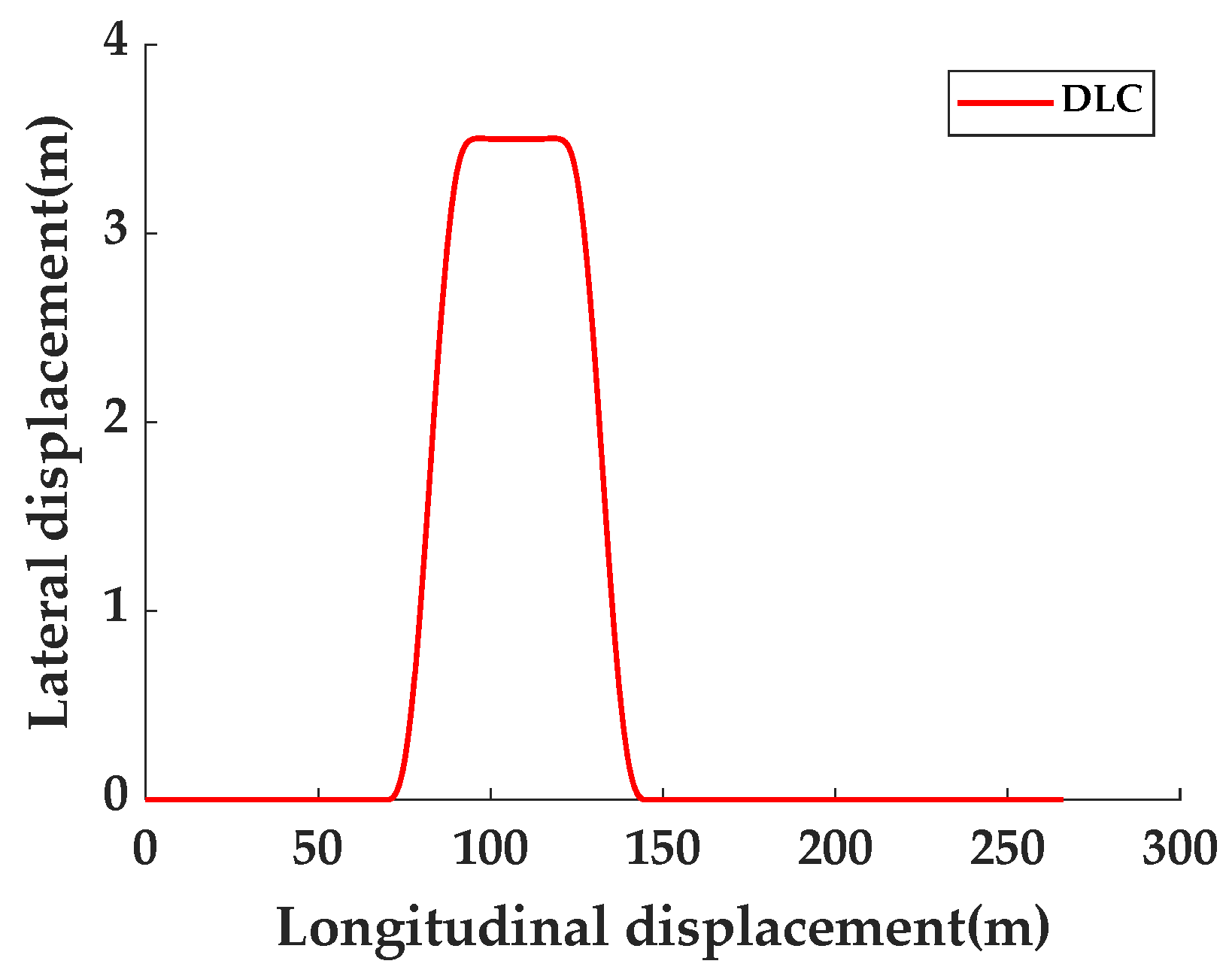
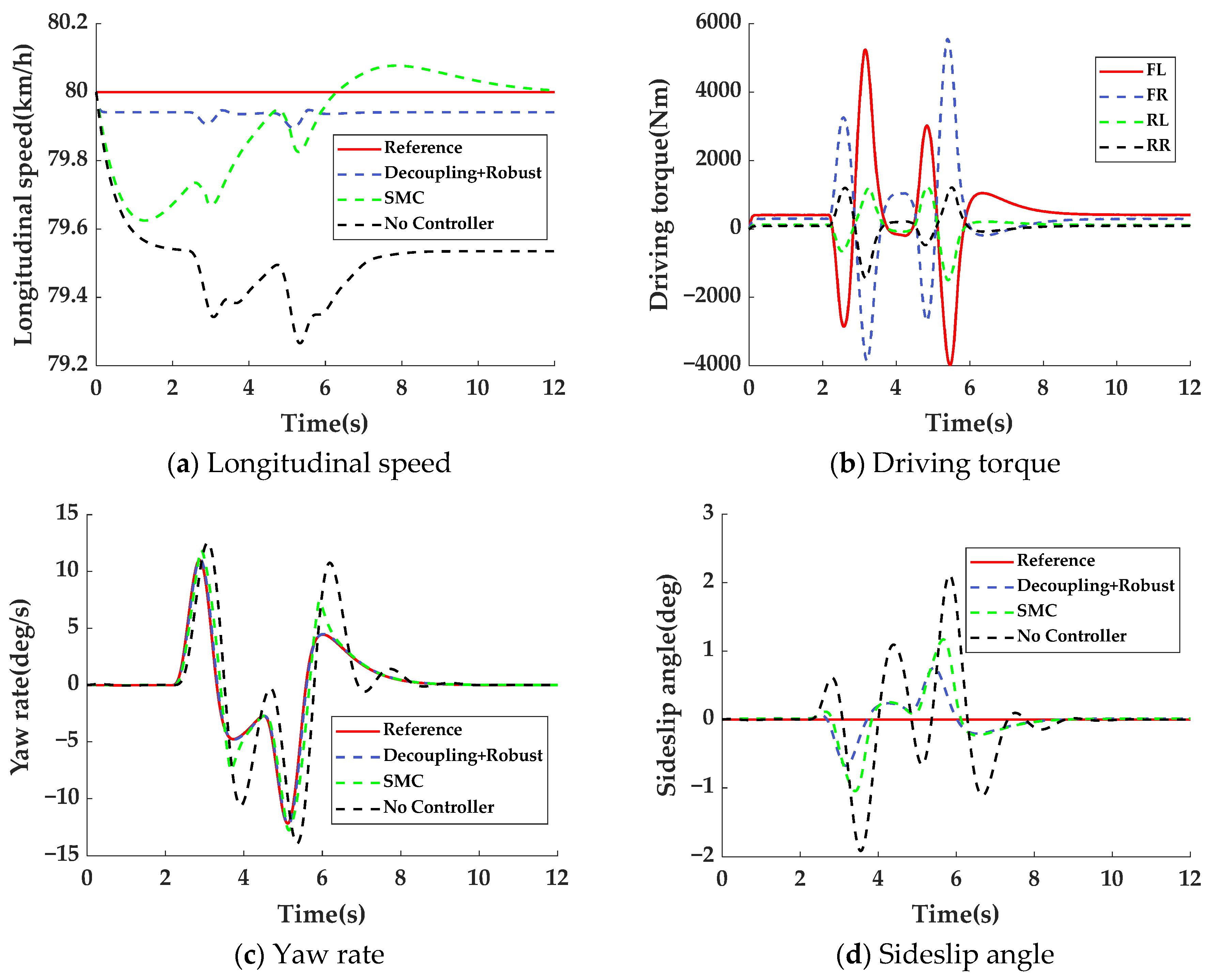
The double-lane change (DLC) condition can simulate the emergency lane change of a vehicle while driving on a highway. The vehicle speed is 80 km/h and the road adhesion coefficient is 0.85. Figure 4 is the DLC simulation path. The results are shown in Figure 5, and the peak error data are presented in

Table 2. Peak errors and comparisons under the DLC condition.

Control Strategy/Optimization Effect	$\Delta {\mathit{v}}_{\mathit{x}}$ (km/h)	$\Delta \mathit{r}$ (deg/s)	$\Delta \mathit{\beta }$ (deg)
Decoupling + Robust	0.1042	0.0663	0.7541
SMC	0.3748	0.8869	1.1707
No Controller	0.7339	1.5364	2.1111
Optimization rate compared with SMC	72.19%	92.52%	35.59%
Optimization rate compared with No Controller	85.81%	95.68%	64.28%

.

It can be seen from Figure 5a that when the steering wheel angle changes, the longitudinal vehicle speeds of vehicles under each control strategy are affected to varying degrees. Analyzing the data in Table 2, it can be seen that the fluctuation amplitude of the longitudinal velocity response curve of Decoupling + Robust is the smallest, and the maximum peak error is only 0.1042 km/h. Compared with other control strategies, the longitudinal velocity of the vehicle is optimized by 72.19% and 85.81%, respectively. This proves that the Decoupling + Robust control strategy has the highest tracking degree for the longitudinal velocity.

Figure 5b shows the curve of the wheel driving torque output by the four in-wheel motors under the control strategy of this paper. It can be seen that the four wheels can achieve torque distribution in the form of driving on one side and braking on the other side. Moreover, the driving torques of the front and rear wheels respond simultaneously. The driving torque of the front wheels is significantly higher than that of the rear wheels, making full use of the adhesion of the tires with a larger axle load, ensuring sufficient lateral adhesion and improving the vehicle driving stability.

It can be seen from Figure 5c and Table 2 that the control strategy proposed in this paper has the best tracking performance for the yaw rate. Its change trend is the most consistent with the expected value and the fluctuation is the smoothest. Compared with other control strategies, the peak error of the yaw rate of the vehicle is optimized by 92.52% and 95.68%. This proves that the vehicle under the Decoupling + Robust control has better stability. It can be seen from Figure 5d and Table 2 that compared with the ideal value curve, the peak errors of vehicles under each control strategy are 0.7541 deg, 1.1707 deg, and 2.1111 deg. The peak error of the vehicle under the Decoupling + Robust control is smaller, proving that the Decoupling + Robust control is effective.

4.3. Fishhook Condition

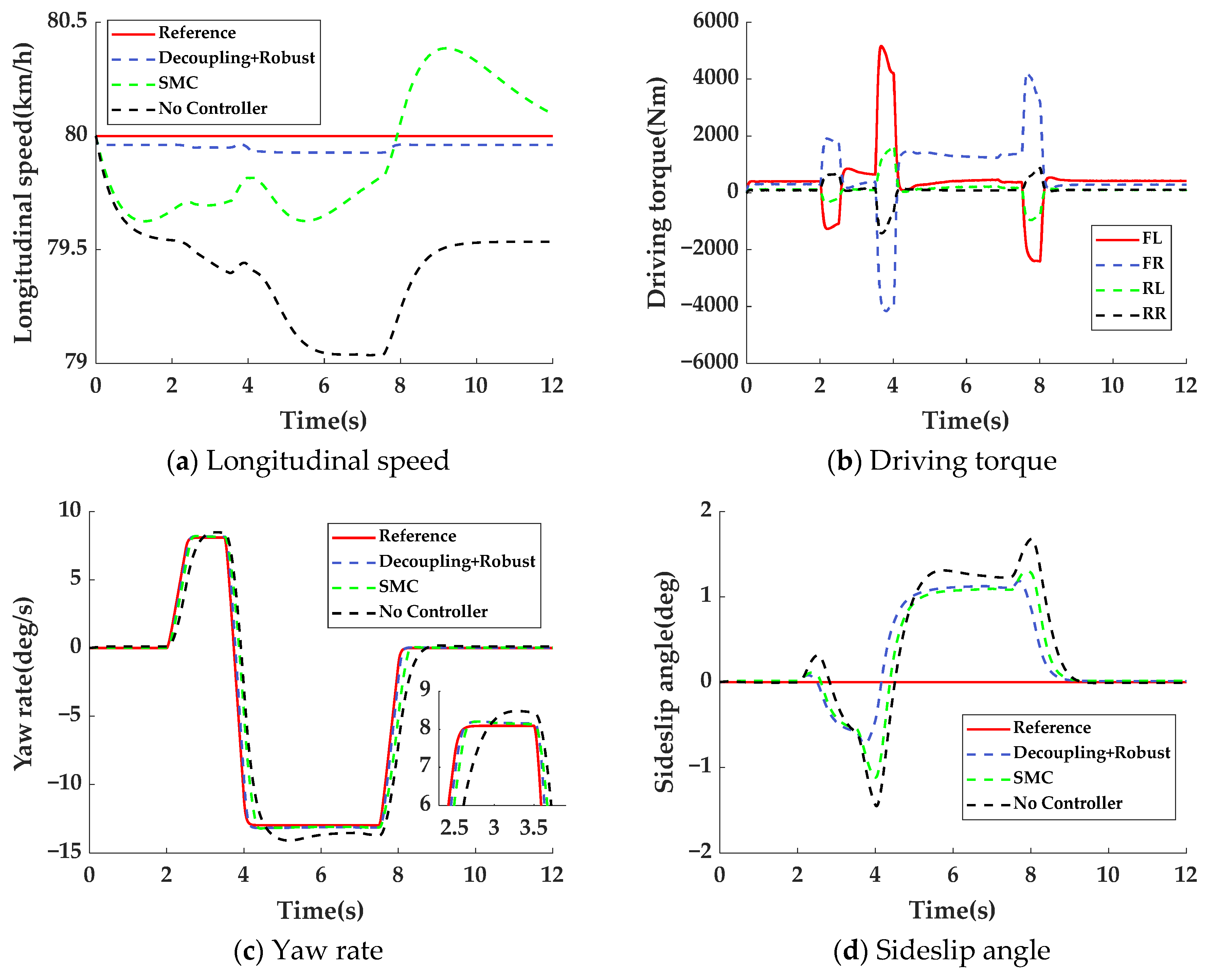
The fishhook condition is used to test the stability of the vehicle under extreme conditions. The vehicle speed is set at 80 km/h and the road adhesion coefficient is 0.85. Figure 6 shows the steering wheel angle under fishhook condition. The results are shown in Figure 7, and the peak error data are presented in

Table 3. Peak errors and comparisons under the fishhook condition.

Control Strategy/Optimization Effect	$\Delta {\mathit{v}}_{\mathit{x}}$ (km/h)	$\Delta \mathit{r}$ (deg/s)	$\Delta \mathit{\beta }$ (deg)
Decoupling + Robust	0.0732	0.1481	1.1817
SMC	0.3854	0.2461	1.3017
No Controller	0.9642	1.1247	1.6783
Optimization rate compared with SMC	81.06%	39.82%	9.22%
Optimization rate compared with No Controller	92.43%	86.83%	29.59%

.

As can be seen from Figure 7a, the vehicles under the SMC and No Controller control strategies failed to closely track the target longitudinal vehicle speed. In contrast, the vehicle under the Decoupling + Robust control had the smallest peak error, with optimizations of 81.06% and 92.43% compared to the vehicles under other control strategies, respectively. This demonstrates that the Decoupling + Robust control strategy has a better control effect.

Figure 7b shows the curve of the wheel driving torque output by the four in-wheel motors under the control strategy of this paper. It can be seen that the four wheels can achieve torque distribution in the form of driving on one side and braking on the other side. Moreover, the driving torques of the front and rear wheels respond simultaneously.

The driving torque of the front wheels is significantly higher than that of the rear wheels, making full use of the adhesion of the tires with a larger axle load, ensuring sufficient lateral adhesion and improving the vehicle driving stability.

From Figure 7c, it can be seen that compared with the ideal value curve, the yaw rate curves of the vehicles under the SMC and No Controller controls both had delays. However, the curve of the Decoupling + Robust control was highly consistent with the ideal value curve. The peak error of the yaw rate of the vehicle was optimized by 39.82% and 86.83% compared to the vehicles under other control strategies, respectively, proving the effectiveness of the Decoupling + Robust control. From Figure 7d and Table 3, it can be seen that the peak errors of the sideslip angle of the center of mass of the vehicles under each control strategy were 1.1817 deg, 1.3017 deg, and 1.6783 deg. The Decoupling + Robust control had the smallest peak error. These results highlight the significantly improved stability of this control system under the fishhook condition.

4.4. Crosswind Interference Condition

To verify whether the controller proposed in this paper can control the uncertain disturbances during the driving process of the vehicle, a crosswind interference test was designed. The test conditions are as follows: The vehicle travels straight into the crosswind area at a speed of 80 km/h. A crosswind is continuously generated from 2 s to 6 s, with a maximum wind speed of 12 m/s. The variation in the crosswind with time is shown in Equation (35). The wind direction is 90° to the driving direction of the vehicle, and the road adhesion coefficient is 0.4. The response curves of the vehicle parameters obtained from the simulation are shown in Figure 8.

$$V=\left\{\begin{array}{ll}0,& 0<t<2\\ 12\left[1-\cos {\displaystyle \frac{5}{2}}\pi \left(t-2\right)\right],& 2\le t<2.2\\ 12,& 2.2\le t<5.8\\ 12\left[1-\cos {\displaystyle \frac{5}{2}}\pi \left(t-6\right)\right],& 5.8\le t<6\\ 0,& t>6\end{array}\right.$$

(35)

As can be seen from Figure 8a and

Table 4. Peak errors and comparisons under the crosswind condition.

Control Strategy/Optimization Effect	$\Delta \mathit{y}$ (m)	$\Delta {\mathit{v}}_{\mathit{x}}$ (km/h)	$\Delta \mathit{r}$ (deg/s)	$\Delta \mathit{\beta }$
Decoupling + Robust	1.1221	0.1189	0.0336	0.5859
SMC	1.9412	0.5624	0.1044	0.6033
No Controller	8.6004	0.9197	0.6502	0.9474
Optimization rate compared with SMC	42.21%	78.86%	67.82%	2.88%
Optimization rate compared with No Controller	86.95%	87.07%	94.83%	38.16%

, under the interference of crosswind, the maximum lateral displacements of vehicles under three different control strategies are 1.1221 m, 1.9412 m, and 8.6004 m, respectively. Analysis shows that the lateral displacement of the vehicle under the No Controller strategy is significantly larger than that of the other two control strategies. If such a situation occurs on a highway, the vehicle has completely deviated from its own lane, posing a great potential hazard to driving safety.

In Figure 8b, compared with other control strategies, the vehicle under the Decoupling + Robust strategy responds faster to the vehicle speed, and the vehicle can follow the desired speed in real time.

By analyzing Figure 8c, it is obvious that when affected by crosswind, the vehicle under the Decoupling + Robust control shows better stability and smaller deviation in yaw rate compared with the vehicles under SMC control and No Controller. In addition, after the crosswind stops, the overshoot of the vehicle under the Decoupling + Robust control is smaller.

By analyzing Figure 8d and Table 4, it can be seen that compared with SMC and No Controller, the peak error of the sideslip angle of the center of mass of Decoupling + Robust is optimized by 2.88% and 38.16%, respectively.

In conclusion, the lateral motion has a relatively small impact on the longitudinal velocity of the vehicle under the Decoupling + Robust control. Moreover, compared with the vehicles under SMC control and No Controller control, this vehicle has a stronger resistance to lateral interference.

5. Conclusions

This study presents a control strategy combining differential geometry decoupling with robust control to solve the coupling issues between steering and drive systems in four-wheel steering distributed drive electric vehicles. The proposed method decouples the three-input-three-output integrated chassis system into three independent subsystems, achieving precise control of longitudinal velocity, yaw rate, and sideslip angle. Taking into account crosswind disturbances during actual driving conditions, robust controllers are designed for the decoupled subsystems to form a hierarchical control architecture.

Co-simulation results using TruckSim and MATLAB/Simulink show that compared to SMC and No Controller cases, the proposed decoupling robust control strategy demonstrates superior performance. In standard DLC and fishhook maneuvers, it maintains a longitudinal speed tracking error within 0.14% while improving the yaw rate by at least 39% and reducing the sideslip angle by 9%. When subjected to crosswind conditions, this method reduces lateral displacement by 42.21% compared to SMC while keeping longitudinal speed deviation at 0.15%, decreasing the yaw rate by 67.82% and lowering the sideslip angle by 2.88%. The strategy effectively enhances vehicle driving stability and safety.

Although the control strategy proposed in this study has been initially verified in offline simulations, future work will focus on real-vehicle testing to obtain more valuable real-world data, thereby making the research more closely aligned with engineering practice.

References

1. Fan, X.; Chen, M.; Huang, Z.; Yu, X. A Review of Integrated Control Technologies for Four In-Wheel Motor Drive Electric Vehicle Chassis. J. Braz. Soc. Mech. Sci. Eng. 2025, 47, 89. [Google Scholar] [CrossRef]
2. Zhang, Y.; Cai, Y.; Sun, X.; Wang, H.; Chen, L.; Chen, T.; Yuan, C. A Review of Coordinated Control Technology for Chassis of Distributed Drive Electric Vehicles. Appl. Sci. 2025, 15, 7175. [Google Scholar] [CrossRef]
3. Liu, S.; Zhang, H.; Wang, S.; Zhao, X. Hierarchical Torque Vectoring Control Strategy of Distributed Driving Electric Vehicles Considering Stability and Economy. Sensors 2025, 25, 3933. [Google Scholar] [CrossRef]
4. Lu, J.; Wang, R.; Wan, C. Intelligent Vehicle Path Tracking and Stability Control Method Based on Extension Coordinated Control of AFS and DYC. IEEE Access 2025, 13, 7353–7365. [Google Scholar] [CrossRef]
5. Zhao, K.; Fan, X.; Huang, Z.; Yu, X.; Wang, L.; Peng, J. A Review of Drive Torque Distribution Control for Distributed Drive Electric Vehicles. Proc. Inst. Mech. Eng. Part D J. Automob. Eng. 2024, 239, 5291–5315. [Google Scholar] [CrossRef]
6. Zhang, C.; Liu, H.; Dang, M. Robust Shared Control for Four-Wheel Steering Considering Driving Comfort and Vehicle Stability. World Electr. Veh. J. 2023, 14, 283. [Google Scholar] [CrossRef]
7. Zhang, J.; Liu, C.; Zhao, J.; Liu, H. Research on Stability Control of Distributed Drive Vehicle with Four-Wheel Steering. World Electr. Veh. J. 2024, 15, 228. [Google Scholar] [CrossRef]
8. Zuo, H.; Ge, P.S.; Wang, Y.; Zhang, T. Research on Integrated Control of Four-Wheel Steering and Direct Yaw Moment for Distributed-Drive Independent Steering Electric Vehicles. J. Chongqing Univ. Technol. (Nat. Sci.) 2025, 39, 12–18. [Google Scholar]
9. Chen, W.; Liang, X.; Wang, Q.; Zhao, L.; Wang, X. Extension Coordinated Control of Four Wheel Independent Drive Electric Vehicles by AFS and DYC. Control Eng. Pract. 2020, 101, 104504. [Google Scholar] [CrossRef]
10. Zakaria, M.S.M.; Singh, A.S.P.; Aras, M.S.M. Direct Yaw Moment-Based Vehicle Stability Control System for Eight-Wheeled Vehicles. Int. J. Dynam. Control 2025, 13, 298. [Google Scholar] [CrossRef]
11. Jin, L.; Wen, Y.; Li, A.; Zhong, Z.; Zhang, F.; Yin, C.; Zhang, Y. Vehicle Stability Control for 4WIS-4WID EV Based on Four-Wheel Steering and Direct Yaw Moment Control. Int. J. Automot. Technol. 2025, 1–14. [Google Scholar] [CrossRef]
12. Lin, F.; Hao, M.; Wang, T.; Wang, X. Research on Lateral Stability Control of Autonomous Vehicles Using Backstepping Sliding Mode Method. J. Mech. Eng. Chin. 2024, 60, 497–506. [Google Scholar]
13. Ni, J.; Hu, J.; Xiang, C. Robust Path Following Control at Driving/Handling Limits of an Autonomous Electric Racecar. IEEE Trans. Veh. Technol. 2019, 68, 5518–5526. [Google Scholar] [CrossRef]
14. Yu, Y.H.; Huang, L.; Li, Y.N.; Zheng, L.; Zhou, J.; Liang, Y.X. Research on Path Tracking Control under Emergency Conditions Based on Dynamic Decoupling. Automot. Eng. 2023, 45, 997–1009. [Google Scholar] [CrossRef]
15. Zhang, Y.T.; Li, F.R.; Tian, H.Q.; Hu, J.B.; Wei, C.; Wu, W. Research on Decoupling Control of Integrated Dynamics System for Unmanned Vehicle Chassis. Automot. Eng. 2021, 43, 1673–1682. [Google Scholar] [CrossRef]
16. Chang, Y.N.; Guo, H.G.; Zhang, C.M. Vehicle Dynamics Model Decoupling Method Based on Neural Network Inverse System. J. Taiyuan Univ. Sci. Technol. 2024, 45, 125–131. [Google Scholar]
17. Liang, Y.X.; Li, Y.N.; Yu, Y.H.; Zheng, L. Longitudinal and Lateral Decoupling Control of Intelligent Vehicles Based on Neural Network Inverse System. J. Hunan Univ. (Nat. Sci.) 2019, 46, 26–35. [Google Scholar] [CrossRef]
18. Wang, F.; Shi, Y.; Chen, Y. Hierarchical MIMO Decoupling Control for Vehicle Roll and Planar Motions with Control Allocation. IEEE Trans. Veh. Technol. 2024, 73, 494–503. [Google Scholar] [CrossRef]
19. Wu, H.; Gao, Q.; Wang, C.; Zhao, W. Decoupling Control of Chassis Integrated System for Electric Wheel Vehicle. Proc. Inst. Mech. Eng. Part D J. Automob. Eng. 2020, 234, 1515–1531. [Google Scholar] [CrossRef]
20. Wang, X.; Sun, W. Trajectory Tracking of Autonomous Vehicle: A Differential Flatness Approach with Disturbance-Observer-Based Control. IEEE Trans. Intell. Veh. 2023, 8, 1368–1379. [Google Scholar] [CrossRef]
21. Gao, S.; Wang, Y.Q.; Wang, Y.H.; Xu, Y.; Zhou, Y.C.; Wang, P.W. Integrated Feedback Linearization Control for Longitudinal and Lateral Dynamics of Intelligent Vehicles. J. Jilin Univ. (Eng. Ed.) 2023, 53, 735–745. [Google Scholar] [CrossRef]
22. Wang, X. Research on Lateral and Longitudinal Coupling Control of Vehicles Based on Differential Flatness. Ph.D. Thesis, Harbin Institute of Technology, Harbin, China, 2025. [Google Scholar]
23. Yao, X.; Zhao, B.; Li, S. Disturbance Observer-Based Tracking Control of High-Speed Trains Under Adhesion Dynamics. IEEE Trans. Autom. Sci. Eng. 2024, 21, 1727–1739. [Google Scholar] [CrossRef]
24. Lyu, S.; Wu, J.F. Robust Controller Design Based on LMI Optimization. Ind. Instrum. Autom. Equip. 2017, 123–125, 128. [Google Scholar]
25. Ge, P.X. Research on Optimal Control of Vehicle Stability System Based on Feedback Linearization. Master’s Thesis, Jilin University, Changchun, China, 2018. [Google Scholar]
Figure 1. Four-wheel steering three-degree-of-freedom vehicle model.
Wevj 16 00673 g001
Figure 2. Tire force diagram.
Wevj 16 00673 g002
Figure 3. Control strategy structure diagram.
Wevj 16 00673 g003
Figure 4. Reference DLC (double-lane change) path.
Wevj 16 00673 g004
Figure 5. Simulation experiment results of the DLC condition.
Wevj 16 00673 g005
Figure 6. Steering wheel angle.
Wevj 16 00673 g006
Figure 7. Simulation experiment results of the fishhook condition.
Wevj 16 00673 g007
Figure 8. Simulation experiment results of the crosswind condition.
Wevj 16 00673 g008