Fault Diagnosis Method of Four-Level Converter Based on Improved Dual-Kernel Extreme Learning Machine

Abstract

To ensure the reliable operation of power converters and prevent catastrophic failures, this paper proposes a novel online fault diagnosis strategy for a four-level converter. The core of this strategy is an optimized multi-kernel extreme learning machine model. Specifically, the model extracts multi-scale features from three-phase output currents by combining Gaussian and polynomial kernels and employs particle swarm optimization to determine the optimal kernel fusion scheme. Experimental validation was performed on an online diagnosis platform for a four-level converter. The results show that the proposed method achieves a high diagnostic accuracy of 99.35% for open-circuit faults. Compared to conventional methods, this strategy significantly enhances diagnostic speed and accuracy through its optimized multi-kernel mechanism.

1. Introduction

As the automotive industry accelerates its critical shift towards electrification, enhancing the efficiency of powertrains is of vital importance. At present, the battery voltage of electric vehicles is mostly 400 or 800 V, and the problem of low energy efficiency limits their performance. In multilevel converters, four-level converters achieve a good balance compared to three-level and five-level converters in terms of the number of devices, device stress, and voltage balance control. It has obvious performance and cost advantages for the future 1200 V electric vehicle battery voltage [1]. The four-level active neutral-point-clamped (4L-ANPC) converter’s minimal switch count simplifies its topology, making it a highly attractive architecture for 1200 V electric vehicle battery voltage [2]. Therefore, the reliability of the 4LANPC converter in practical applications is crucial for normal and safe operation [3,4].

However, the reliability of the 4L-ANPC converter is challenged by susceptibility of its power semiconductor devices to failures, especially open-circuit faults (OCFs). OCFs may lead to an increase in the harmonic of the terminal voltage or current, which can have a long-term damaging effect on inverter-supplied devices such as transformers or motors [5,6]. Therefore, the system should have fast OCF diagnosis capability to prevent serious consequences.

In recent years, many studies have been devoted to switching OCF diagnosis methods for two-level or three-level converters, which are mainly categorized into model-based and data-driven methods. Model-driven methods compare the state-observed response with the actual response to obtain the residual signal and then determine whether a fault has occurred or not. Overall, model-driven fault diagnosis methods are efficient and widely used, but they rely too much on mathematical models [7].

In contrast, data-driven approaches, which have gained significant attraction, use machine learning to learn directly from operational data. For instance, some studies have successfully applied techniques like artificial neural networks or support vector machines for OCF diagnosis [8,9]. In addition, machine learning methods require parameter updating, have high sample requirements, and are slow, making it difficult to realize online fault diagnosis of power electronic converters.

The extreme learning machine (ELM) is a special kind of single hidden layer neural network, which is characterized by network simplicity and fast training [10]. However, the ELM algorithm uses linear feature mapping, which is often strained for more complex nonlinear pattern recognition tasks. The kernel extreme learning machine (KELM) introduces the kernel function into the traditional ELM, which implicitly maps the low-dimensional linearly indivisible samples to the high-dimensional or even infinite-dimensional feature space through the simple kernel function. Therefore, the nonlinearly divisible problem can transform into a linearly divisible problem in the feature space [11]. The KELM has excellent learning ability for complex classification problems with fast model training, which is very suitable for online fault diagnosis. In addition, while artificial intelligence (AI) methods have been increasingly applied for fault diagnosis in various multilevel converters, such as the three-level NPC and modular multilevel converters [12], their specific application to the 4LANPC converter topology remains a less explored area in the existing literature. This presents a clear opportunity for developing advanced, data-driven diagnostic models tailored to the unique characteristics of the 4LANPC converter, which this study aims to address.

For the above considerations, this paper proposes an online diagnosis method for switching OCFs in the 4LANPC converter using an improved dual-kernel extreme learning machine (DKELM). Based on the measured three-phase output currents, Gaussian kernel and polynomial kernel are utilized to extract multi-scale features, respectively, and then a fast and effective high-accuracy fault diagnosis model is established by the KELM learning mechanism. In particular, the fusion scales of the Gaussian kernel and polynomial kernel are optimized by particle swarm optimization (PSO). The experimental results show that it can effectively diagnose OCFs with an accuracy rate higher than 99.35%. It is noticed that the proposed method only focuses on single open-circuit faults.

The main contributions are as follows:

• An OCF diagnosis method of 4LANPC converter based on the DKELM technique is proposed, which enriches the research work on artificial intelligence methods, empowering fault diagnosis of the 4LANPC converter.
• The network structure of DKELM is developed, which is realized by the PSO method that prefers the fusion scales of the Gaussian kernel and polynomial kernel.
• The experimental results show that this method has good accuracy of fault diagnosis and is simple to implement.

The rest of the paper is organized as follows. The proposed methodology is presented in Section 2. Section 3 presents experimental setup and validation. Finally, Section 4 presents the conclusion.

2. Proposed Techniques

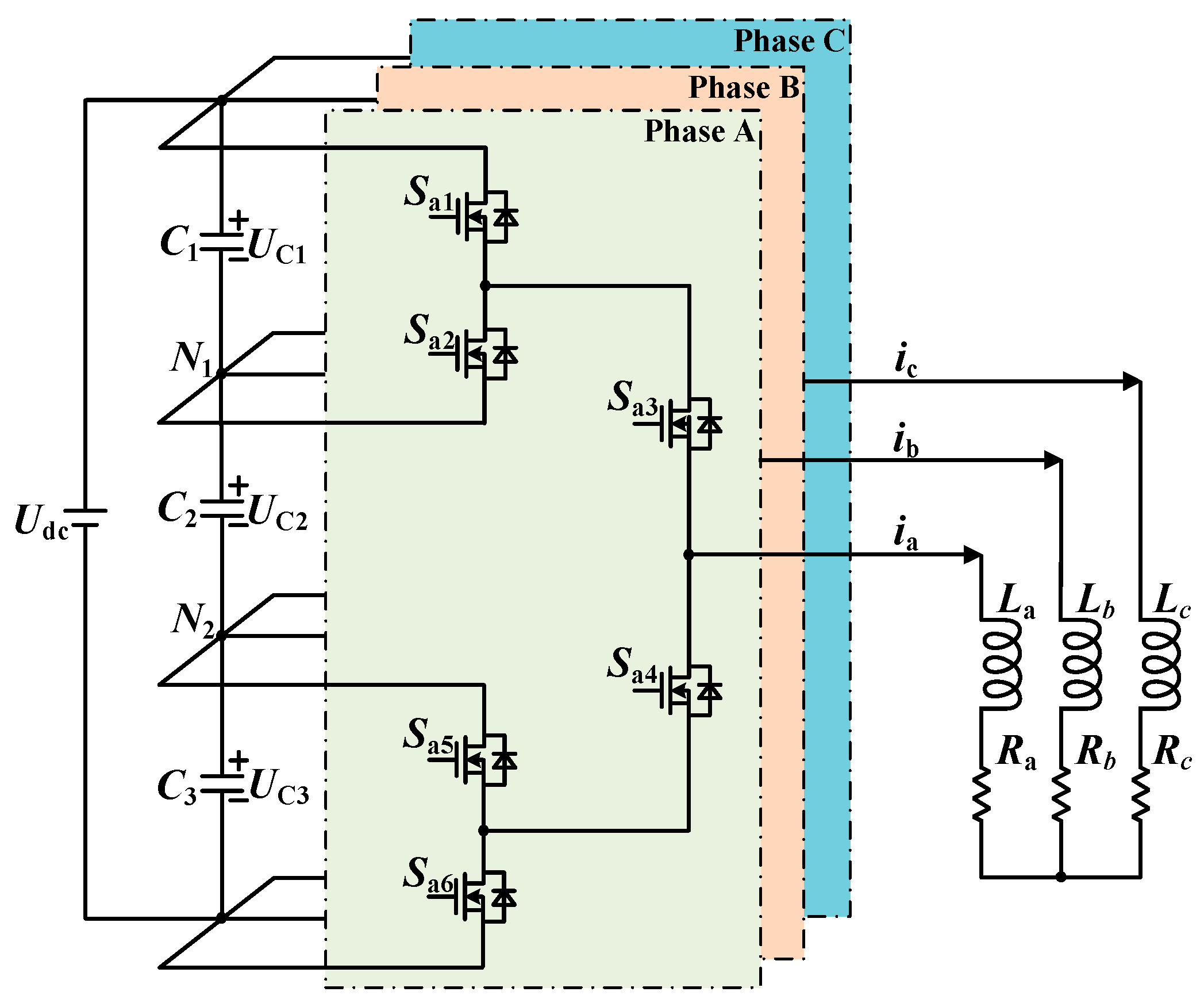
The considered 4LANPC converter topology is given in Figure 1. Functionally, this topology generates a four-level AC voltage output from a single DC input. The DC link voltage is divided by three series capacitors creating the neutral points N1 and N2. By controlling the switching states of the power semiconductors in each phase leg, the output terminal can be connected to different voltage potentials, thereby synthesizing a smooth, high-quality AC waveform with low harmonic distortion. 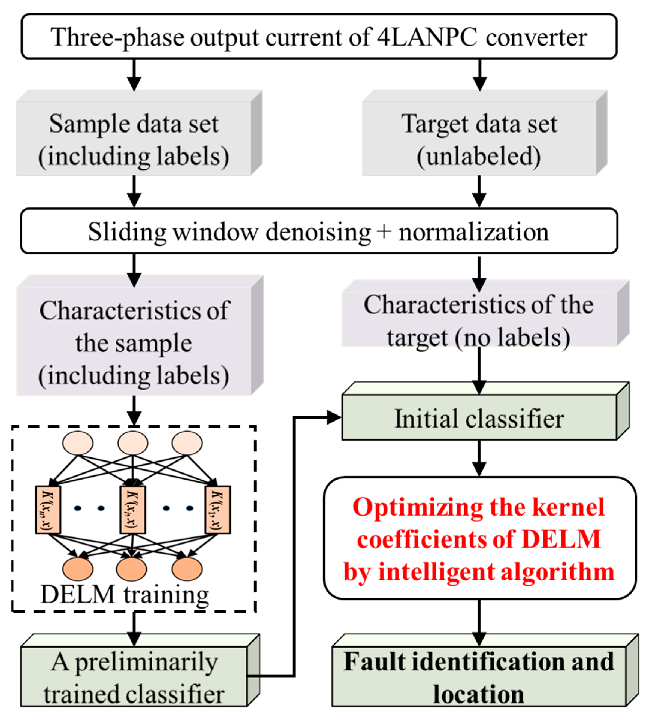The OCF labels are defined in Table 1. The proposed OCF diagnostic model for the 4LANPC converter contains the DKELM method and PSO algorithm. The PSO method is used to optimize the fusion scales of the Gaussian kernel and polynomial kernel. The implementation flow of the proposed fault diagnosis method is shown in Figure 1.

Figure 1. Topology of the 4LANPC converter.

Table 1. Fault states and labels.

Switch	Fault Label	Switch	Fault Label
Sa1	1	Sb5	11
Sa2	2	Sb6	12
Sa3	3	Sc1	13
Sa4	4	Sc2	14
Sa5	5	Sc3	15
Sa6	6	Sc4	16
Sb1	7	Sc5	17
Sb2	8	Sc6	18
Sb3	9	No Fault	19
Sb4	10	-	-

2.1. DKELM Network

The ELM has $n$ input neurons, $L$ hidden layer neurons, and $m$ output neurons. The activation function is $p(x)$, and the mathematical model is denoted as

$$H\beta =T,$$

(1)

where $H={[h{(x_1)}^T,\dots ,h{(x_N)}^T]}^T=\left[\begin{array}{ccc}p(w_1·x_1+b_1)& \dots & p(w_L·x_1+b_L)\\ ⋮& \ddots & ⋮\\ p(w_1·x_N+b_1)& \dots & p(w_L·x_N+b_L)\end{array}\right]$. $w_i={[w_{i1},w_{i2},\dots ,w_{in}]}^T$ denotes the input weights connecting the $i$-th hidden layer neuron to the input layer neuron; $b_i$ is the bias value of the $i$-th hidden layer neuron; $x_i={[x_{i1},x_{i2},\dots ,x_{in}]}^{\mathrm{T}}\in R^n$ is the input vector and is the corresponding desired output vector. This equation represents the fundamental model of the ELM. It establishes a linear relationship where H is the hidden layer output matrix, β is the matrix of output weights connecting the hidden layer to the output layer, and T is the matrix of target outputs. The primary objective of the ELM training process is to determine the optimal output weights β by solving this linear system. The procedures of proposed fault diagnosis method for the 4L-ANPC converter are presented in Figure 2.

Figure 2. The proposed fault diagnosis method for the 4L-ANPC converter.

$\beta ={[{\beta }_1,{\beta }_2,\dots ,{\beta }_L]}^T$ refers to the weight matrix between the output layer and the hidden layer, and $T={[t_1,t_2,\dots ,t_N]}^T$ is the expected output matrix of training sample.

The minimum paradigm solution of the ELM $\widehat{\beta }$ is

$$\widehat{\beta }=H^{+}T,$$

(2)

where $H^{+}$ denotes the Moore–Penrose generalized inverse of the hidden layer output matrix $H$ [13].

Define the kernel matrix of the ELM according to the Mercer condition, which is denoted as

$${\mathrm{\Omega }}_{\mathrm{ELM}}=hh==H{H}^{\mathrm{T}}:{\mathrm{\Omega }}_{{\mathrm{ELM}}_{i,j}}=h(x_i)·h(x_j)=K(x_i·x_j).$$

(3)

Then the output of the KELM model is expressed as

$$\begin{array}{cc}\hfill f(x)& =h(x)\beta =h(x)H^T{({\displaystyle \frac{1}{c}}+H{H}^T)}^{-1}T\hfill \\ \hfill & =\left[\begin{array}{c}K(x,x_1)\\ ⋮\\ K(x,x_N)\end{array}\right]{({\displaystyle \frac{1}{c}}+{\mathrm{\Omega }}_{ELM})}^{-1}T\hfill \end{array}.$$

(4)

where f(x) represents the model’s final predictive output for a new input sample x. The expression calculates this prediction by leveraging the kernel function, which is implicitly contained within the h(x)H^T term to measure the similarity between the new input and all training samples. This information is then weighted by the learned parameters of the model, represented by the term (1/c + HH^T)⁻¹T. Here, c is the regularization factor, which is a crucial hyperparameter that helps prevent the model from overfitting to the training data, thereby improving its generalization performance on unseen data.

The proposed DKELM applies both Gaussian kernel function and polynomial kernel function to construct the new kernel function method, which is constructed as

$$\begin{array}{cc}\hfill K^{\prime }(x_i,x_j)& ={\displaystyle \sum _{n=1}^2{a}_n{K}_n(x_i,x_j)}\hfill \\ \hfill & =(a_1(\exp \{-{‖x_i-x_j‖}^2/2g^2\}),\hfill \\ \hfill & +{(a_2⟨x_i,x_j⟩+r)}^d)\hfill \end{array}$$

(5)

where a₁ and a₂ are the dual-kernel function coefficients, a₁ +a₂ = 1. In order to better integrate the performance of the dual-kernel function, this paper optimizes the dual-kernel function coefficients by the intelligent optimization algorithm.

The proposed DKELM constructs a new kernel by linearly combining the Gaussian kernel and the polynomial kernel. This specific combination is chosen to leverage the complementary strengths of both functions. The Gaussian kernel is a local kernel function, making it highly effective at learning complex, local nonlinear relationships within the fault data. Conversely, the polynomial kernel is a global function, which is better suited for capturing the global structure and trends in the feature space. The particle swarm optimization (PSO) is then employed to determine the optimal fusion coefficients, ensuring the model is perfectly tailored to the specific characteristics of the OCF signals.

2.2. PSO Algorithm

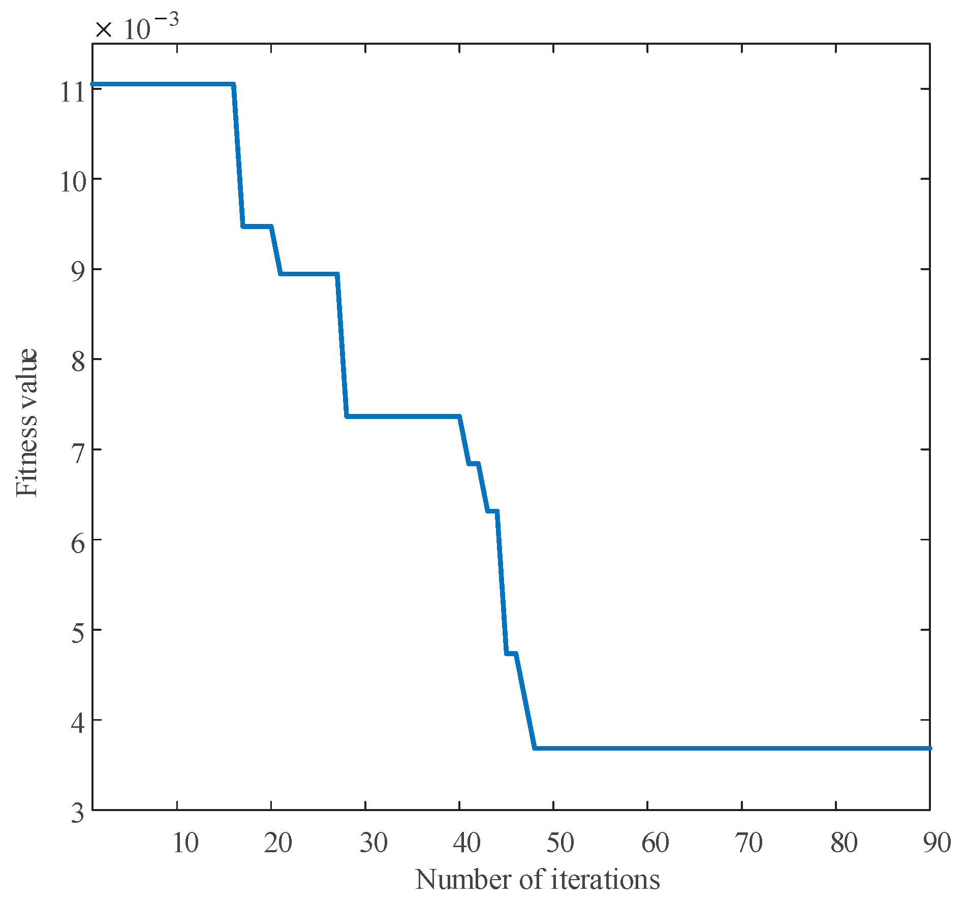
The PSO algorithm is an evolutionary computation technique. The basic idea is to find the optimal solution through collaboration and information sharing between individuals in a population of particles [14]. It is simple and easy to implement and does not have a lot of parameter adjustments. In this paper, the Gaussian kernel and polynomial kernel fusion scales a1 and a2 in the DKELM method are mapped as particles. The minimum training model error is taken as the fitness function, and the PSO algorithm is adopted for optimization. The iteration ends when the absolute error is less than 0.01. The pseudo-code of the PSO method [15] is shown in Algorithm 1.

Algorithm 1: PSO method

Input: The regularization coefficient c of KELM and the Gaussian kernel hyperparameter g

Output: The preferred c and g

1: FOR each particle i

2: FOR each dimension d

3: Initialize position xid randomly within permissible range

4: Initialize velocity vid randomly within permissible range

5: END FOR

6: END FOR

7: Iteration k = 1

8: DO

9: FOR each particle i

10: Calculate fitness i

11: IF the fitness value is better than $p_{id,pbest}^k$ in history

12: Set current fitness value as the $p_{id,pbest}^k$

13: END IF

14: END FOR

15: Choose the particle having the best fitness value as the $p_{d,gbest}^k$

16: FOR each particle i

17: FOR each dimension d

18: Calculate velocity according to the equation

19: Calculated by Equation (6)

20: Update particle position according to the equation

21: Calculated by Equation (7)

22: END FOR

23: END FOR

24: k = k + 1

25: WHILE maximum iterations or minimum error criteria are not attained

In the context of our DKELM model, determining the optimal fusion scales for the Gaussian and polynomial kernels is a non-trivial task. A manual or grid-search approach would be computationally expensive and may not find the global optimum. PSO provides an efficient and robust mechanism to intelligently search this parameter space, making it a highly appropriate choice for fine-tuning the kernel fusion in our fault diagnosis framework. The Gaussian kernel and polynomial kernel fusion scales a1 and a2 in the DKELM method are mapped as particles in this paper. The minimum training model error is taken as the fitness function, and the PSO algorithm is adopted for optimization. The iteration ends when the absolute error is less than 0.01.

$$v_{id}^{k+1}=w{v}_{id}^k+c_1{r}_1(p_{id,pbest}^k-x_{id}^k)+c_2{r}_2(p_{d,gbest}^k-x_{id}^k),$$

(6)

$$x_{id}^{k+1}=x_{id}^k+v_{id}^{k+1},$$

(7)

where $v_{id}^k$ is the velocity vector of particle i in the d-th dimension in the k-th iteration, $x_{id}^k$ is the position vector of particle i in the d-th dimension in the k-th iteration, $p_{id,pbest}^k$ is the historical optimal position of particle i in the d-th dimension in the k-th iteration, and $p_{d,gbest}^k$ is the historical optimal position of the population in the d-th dimension in the k-th iteration. d = 1, 2, …, D, D is the particle dimensionality, k is the number of iterations, and w is the inertia weight. c₁ is the individual learning factor, c₂ is the population learning factor, and i = 1, 2, …, N, N is the particle population size.

Equation (6) is the core mechanism of the PSO algorithm, defining how each particle adjusts its velocity in the search space. This adjustment is guided by three conceptual influences: the particle’s own momentum, the pull toward its individual best-known position, and the pull toward the entire swarm’s best-known position. The relative strengths of these influences are controlled by key parameters defined in the variable list, such as the inertia weight and the cognitive and social learning factors. The proper tuning of these parameters is critical to the algorithm’s performance, as it balances the need for global exploration with local exploitation, which directly impacts the convergence speed and the quality of the result.

3. Experimentation Results and Discussion

3.1. Experimental Acquisition and Processing

The software experiment platform is a desktop computer with a central processor i9-13900 and matlab2022a. The DC power supplies 50 V, and the load is 10 Ω. The resistor and inductor are connected in series to create a nonlinear load. DSP28379D manages the operation of the 4L-ANPC converter with a variable-carrier PWM strategy. MATLAB 2022a captures the data collected by the high-precision sensor-integrated board in real time to diagnose the 4L-ANPC converter’s switch faults online, as shown in Figure 3. To ensure our dataset is representative of real-world signal characteristics rather than just idealized waveforms, we operate each fault category independently for 1 h. Although the macroscopic experimental conditions were kept constant, the operating system introduces small, random variations that are inherent in a real-world system, such as fluctuations in sensor noise and microsecond-level timing differences in switch actions. This significantly increases the data’s diversity and variability.

Figure 3. Experimental platform.

Taking a phase as an example, the collected three-phase output current is shown in Figure 4. A detailed analysis of these waveforms reveals the distinct and challenging characteristics of the fault data. Figure 4a displays the current signature for fault label F1. A key characteristic here is that the current in one phase is severely distorted; its positive peak value is significantly attenuated, reaching only approximately half of the amplitude seen in the healthy phases. In contrast, Figure 4b, which corresponds to fault label F2, exhibits a different distortion pattern. Here, the peak current values are unstable, showing noticeable amplitude fluctuations from one cycle to the next across the phases. The OCF experiment is achieved by not sending the switch tube drive signal.

Figure 4. Partial fault characterization data for (a) fault label F1 and (b) fault label F2.

The fault waveforms show that the collected data contains noise, which is fatal to the modeling training of artificial intelligence techniques. To address this, this paper adopts a sliding window averaging method for data preprocessing. A window size of K = 300 was empirically chosen as an optimal trade-off. It is large enough to effectively suppress the high-frequency noise while being small enough to preserve the crucial transient characteristics inherent to the fault events.

Ac, Pr, Recall, and F1 are introduced to evaluate the diagnostic results, as shown in Equations (8)–(11).

$$\mathrm{Ac}={\displaystyle \frac{\mathrm{T}1+\mathrm{T}2}{\mathrm{T}1+\mathrm{T}2+\mathrm{F}0+\mathrm{F}2}},$$

(8)

$$\mathrm{Pr}={\displaystyle \frac{\mathrm{T}2}{\mathrm{F}2+\mathrm{T}2}},$$

(9)

$$\mathrm{Recall}={\displaystyle \frac{\mathrm{T}2}{\mathrm{F}0+\mathrm{T}2}},$$

(10)

$$\mathrm{F}1=2\times {\displaystyle \frac{\mathrm{Pr}\times \mathrm{Recall}}{\mathrm{Pr}+\mathrm{Recall}}}$$

(11)

where T1 is the number of true-negative classes, F0 is the number of false-negative classes, T2 is the number of true-positive classes, and F2 is the number of false-positive classes.

3.2. Diagnostic Results

This paper splits the data into training set and testing set by 7:3. The PSO algorithm is used to choose the fusion scales of the Gaussian kernel and polynomial kernel of DKELM with the fault diagnosis accuracy as the PSO fitness function. Particle population is 100, and the maximum number of iterations is 90. The optimized a1 = 0.62 and a2 = 0.38. Figure 5 shows the iteration process of the PSO algorithm. After approximately 40 iterations, the curve begins to flatten and approach saturation. This plateau is a typical characteristic of a successful optimization process and signifies that the algorithm has converged. At this stage, the swarm has transitioned from a broad exploration to a fine-tuned exploitation of the best-found solution. This saturation confirms that the PSO has reliably found a stable solution for the fusion coefficients.

Figure 5. Optimization iteration process of the PSO algorithm.

The OCF diagnosis experiment of the 4LANPC converter is launched with the preferred dual-kernel function coefficients. For each category of OCFs and healthy operation, the experiments are repeated 100 times through the test platform, and the test results are shown in Figure 6. The experimental results show that the proposed method is able to achieve zero error in recognizing the fault-free healthy operation state. However, the proposed method has five and seven false alarms for the fault states ‘F12’ and ‘F15’, respectively, which is a maximum false alarm rate of 7%. But the overall diagnostic accuracy of the proposed method is as high as 99.36%, and the false alarm rate is lower than 0.5%, which is excellent in terms of accuracy and robustness.

Figure 6. Diagnostic results.

It is noteworthy that in Figure 6, the ‘True labels’ are largely obscured by the ‘Diagnostic labels’. This is a direct visual representation of the model’s high performance. The ‘Diagnostic labels’ are plotted over the ‘True labels’, and the near-perfect overlap between the two signifies that the model’s predictions are highly consistent with the ground truth.

Considering the problem of model overfitting, several standard and strict methods have adopted:

(1)

Strict train–test split: We adhered to the golden rule of machine learning by strictly partitioning the dataset into training and testing sets. All model training and optimization were performed exclusively on the training set. The final reported performance metrics, such as the 99.36% accuracy in Table 2 and Figure 7, are evaluated on the unseen test set. Achieving high accuracy on unseen data is the most direct evidence that the model generalizes well and is not overfitted.

Table 2. Results of comparison experiment.

Methods	Ac	Pr	Recall	F1	Diagnostic Time (s)
CNN	0.9095	0.8949	0.9090	0.9021	2.46
LSTMNN	0.9194	0.9779	0.9195	0.8982	2.13
GRU	0.9347	0.9132	0.9329	0.9238	1.78
Proposed method	0.9936	0.9937	0.9937	0.9937	0.53

Figure 7. Comparative test diagnostic results for (a) CNN; (b) LSTMNN; (c) GRU; (d) proposed method.

(2)

Robust performance evaluation: The diagnostic results we report are based on statistical data from 100 independent experiments, which is not the best result of a single run. This evaluation approach ensures the stability and reliability of our conclusions, avoiding potentially misleading results due to chance.

4. Comparative Experiment and Discussion

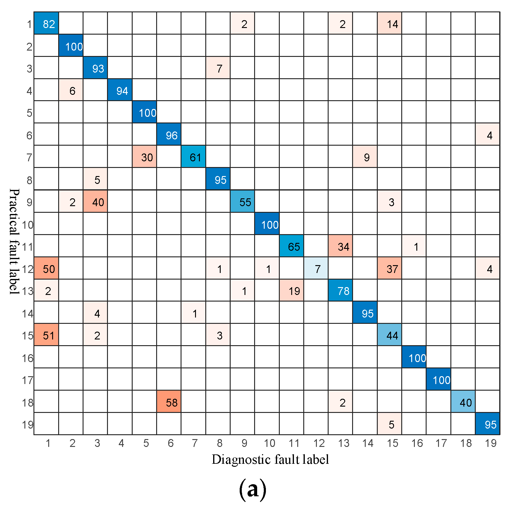
In order to verify the diagnostic performance of the proposed method, the comparison experiment is carried out. The compared algorithms include convolutional neural network (CNN), long short-term memory neural network (LSTMNN), and gated recurrent unit (GRU).

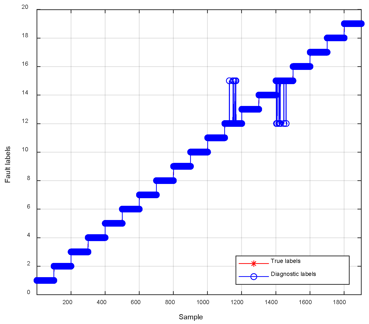
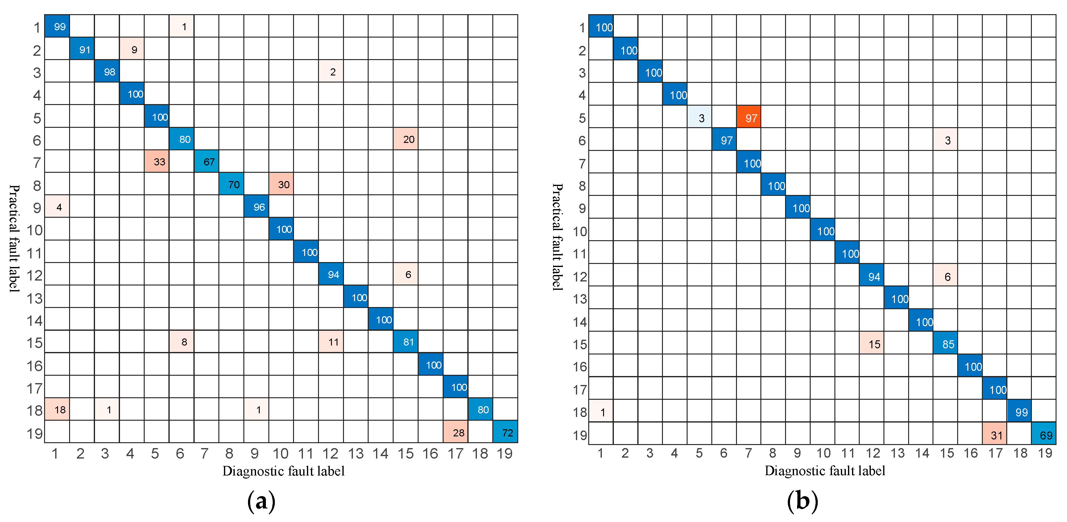
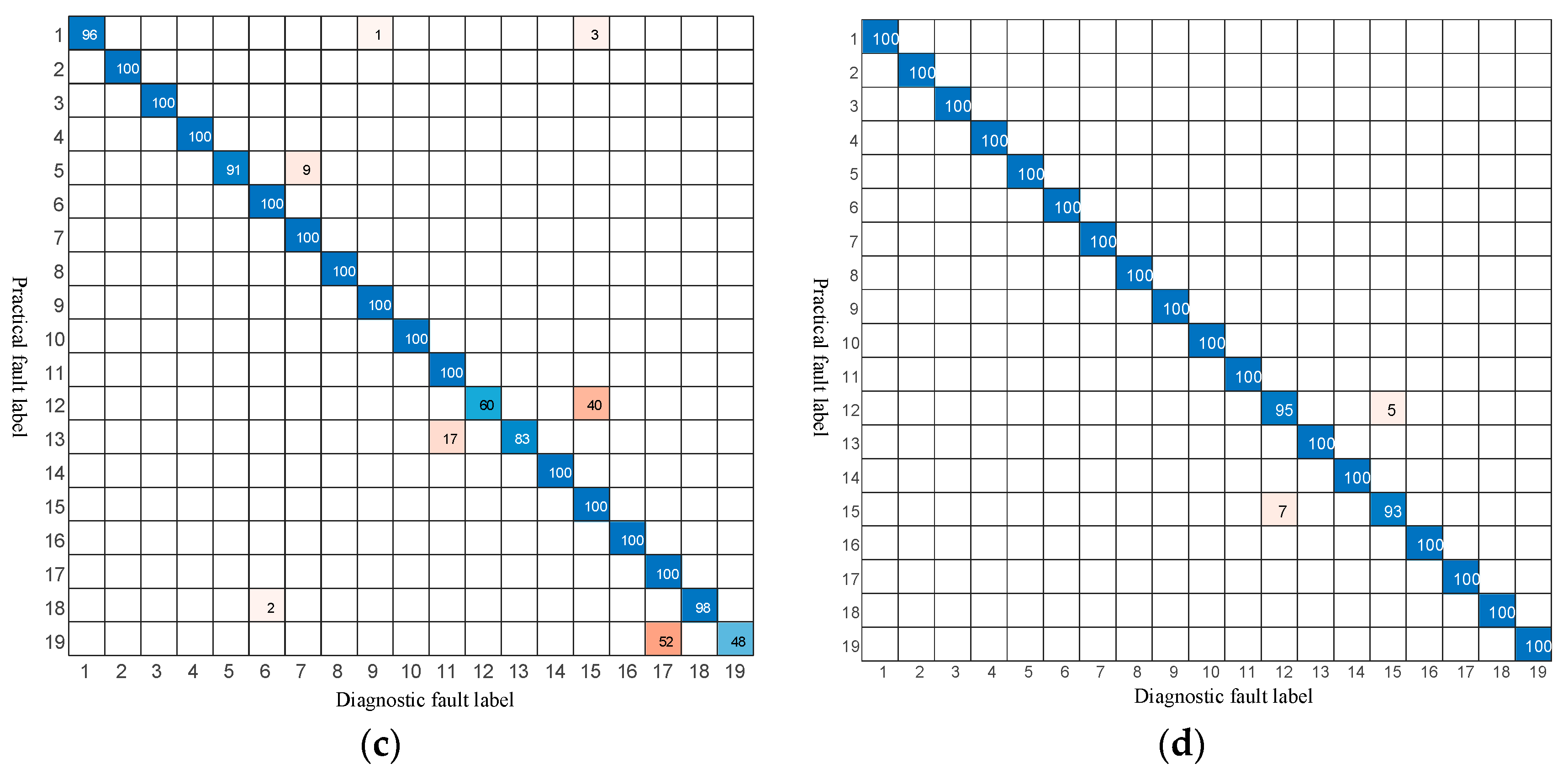
To verify robustness and accuracy, each OCF of the 4LANPC converter was tested 100 times, and the experimental results are shown in Figure 7. Table 2 reports statistical errors. To ensure a fair and direct comparison, all models were trained and tested using the exact same dataset, with the identical 7:3 training–testing split.

Overall, the diagnostic accuracies from low to high are as follows: CNN < LSTM < GRU < proposed method. Different faults are difficult to distinguish using traditional data-driven methods. For example, the diagnostic errors of the CNN method for faults ‘F6’, ‘F7’, ‘F8’, ‘F18’, and ‘F19’ are more than 20%, while the diagnostic errors of LSTM for fault ‘F5’ is more than 20%. The diagnostic accuracy of LSTM for fault ‘F5’ is only 3%, and the diagnosis error of GRU for faults ‘F12’ and ‘F19’ is more than 40%. In contrast, the proposed method is characterized by high accuracy, good robustness, and fast diagnosis for different faults, which illustrates the great potential of the proposed method in practical applications.

The key difference lies in their approach to feature extraction. CNNs excel at identifying local patterns in the current waveform, while LSTMNN and GRU are designed to capture its long-term temporal dependencies. In contrast, our proposed DKELM method is architected to do both simultaneously. Its dual-kernel design synergistically combines a Gaussian kernel to learn subtle local fault features and a polynomial kernel to capture the global structure of the data. This combined local–global learning capability is the primary reason for its enhanced diagnostic accuracy.

As shown in Figure 7a, the CNN model exhibits significant misclassification for several faults, particularly confusing ‘F6’, ‘F7’, and ‘F8’. This suggests that while CNNs are effective feature extractors, they may struggle to differentiate between faults whose current waveforms share similar local patterns. The performance of the recurrent networks, LSTMNN and GRU, is better but still shows notable weaknesses. For instance, LSTMNN almost completely fails to identify fault ‘F5’, indicating a potential difficulty in capturing the specific temporal dependencies of this fault.

In stark contrast, the confusion matrix for our proposed method displays a nearly perfect diagonal line, with only minimal off-diagonal entries. This visually confirms its superior accuracy and robustness across almost all fault types. This enhanced performance can be directly attributed to DKELM’s synergistic use of Gaussian and polynomial kernels, which allows the model to simultaneously learn both the subtle, localized features and the broader, global temporal structures within the fault data.

It is clarified that the current study is specifically focused on single OCFs in power semiconductor devices. The model’s effectiveness in diagnosing other types of faults, such as short-circuit faults, multiple concurrent faults, or intermittent faults caused by drive signal errors, has not yet been systematically validated. Extending the diagnostic framework to encompass a broader range of fault categories will be a key direction for our future research.

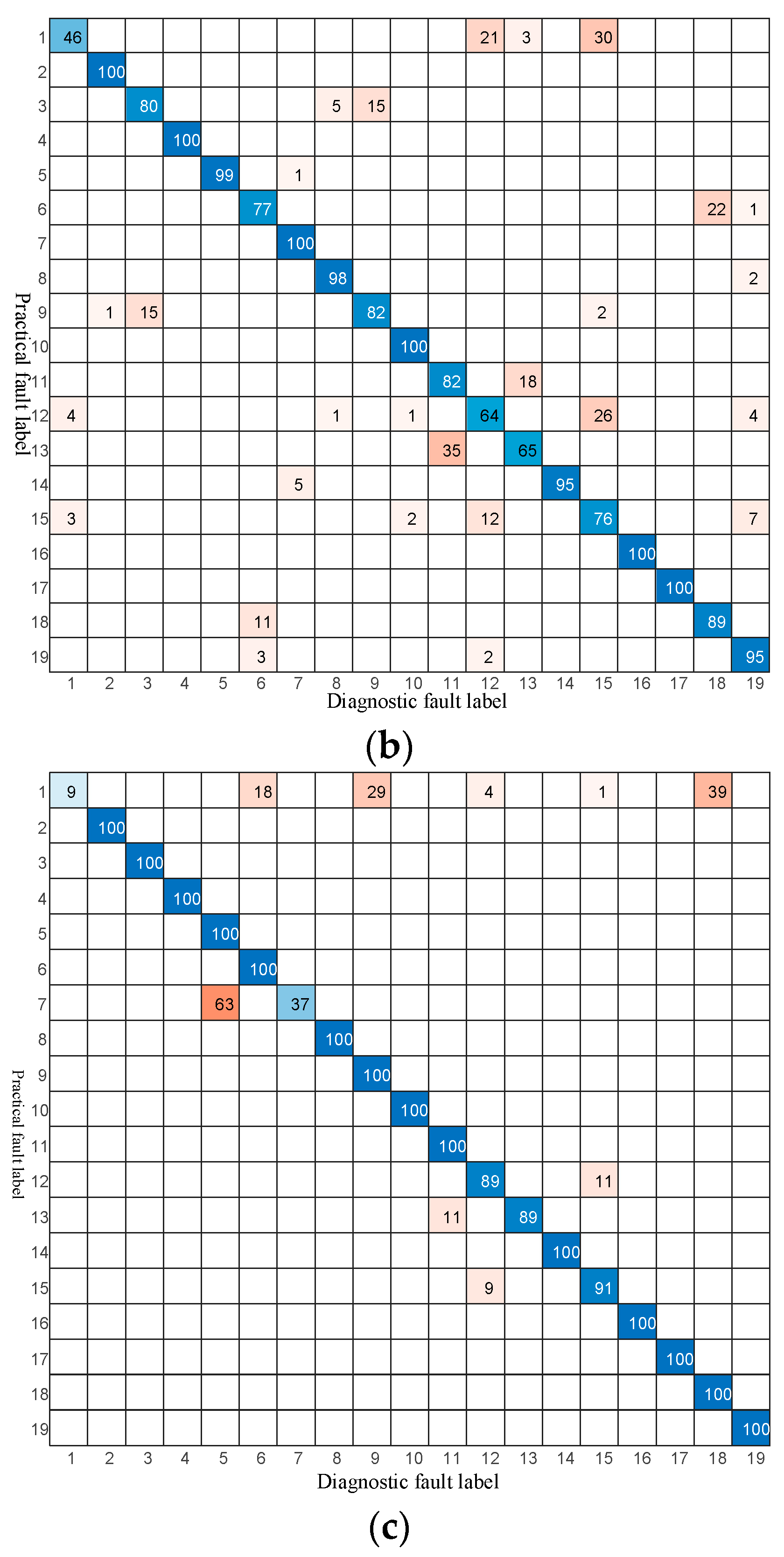
To further validate the superiority of the proposed method, additional comparative experiments were conducted against three classical diagnostic algorithms, including ELM with a polynomial kernel, ELM with a Gaussian kernel, and the SVM method, as shown in Figure 8. As illustrated in Figure 8a, the ELM with polynomial kernel exhibits a relatively scattered confusion matrix, with several misclassifications observed among fault types 1, 5, 10, and 13. The overall recognition performance remains unsatisfactory for closely related fault categories. In Figure 8b, the ELM with Gaussian kernel shows a notable improvement in diagonal dominance, yet certain fault classes such as labels 3, 9, and 14 still suffer from misidentification due to insufficient nonlinear feature representation. The SVM method, as shown in Figure 8c, achieves higher classification accuracy than both ELM variants, but misclassifications are still present in cases with overlapping fault signatures.

Figure 8. The diagnostic results of other comparison algorithms: (a) ELM with polynomial kernel; (b) ELM with Gaussian kernel; (c) SVM method.

In contrast, the proposed method achieves a nearly perfect diagonal distribution in its confusion matrix, indicating more accurate and stable fault identification across all categories. This improvement demonstrates the method’s stronger generalization and robustness to inter-class similarity, benefiting from its adaptive feature extraction and optimized network structure.

5. Conclusions

In this work, an OCF diagnosis approach is presented for 4LANPC converters. By utilizing the measured three-phase output currents, multi-scale features are extracted through Gaussian and polynomial kernels, which are subsequently integrated into an improved DKELM to construct a fast and accurate diagnosis model. The optimal fusion of Gaussian and polynomial kernel scales is determined using a PSO algorithm. The key advantage of this approach is its superior accuracy and robustness, as the dual-kernel structure effectively captures complex fault features that challenge other methods. However, a significant limitation of the current study is its exclusive focus on single open-circuit faults. The model’s effectiveness against other types, such as short-circuits or multiple concurrent faults, has not been validated. Experimental verification is conducted on a laboratory-built online diagnosis platform, and the results demonstrate that the proposed method achieves an OCF detection accuracy exceeding 99.35%. The contribution is summarized as follows:

• A novel machine-learning-based OCF diagnosis method for 4LANPC converters, advancing the application of artificial intelligence in converter fault diagnosis.
• The introduction of DKELM into power electronic fault diagnosis, with PSO-based optimization of multi-kernel fusion scales.
• High diagnostic accuracy and rapid inference capability, highlighting the potential of the proposed method for industrial implementation.