The Design Optimization of a Harmonic-Excited Synchronous Machine Operating in the Field-Weakening Region

Abstract

In this paper, the optimization of a harmonic-excited synchronous machine (HESM) is carried out. A two-phase harmonic exciter winding of the HESM provides brushless excitation and sufficient starting torque at any rotor position. The HESM under consideration is intended to be used for applications requiring speed control, especially in the field-weakening region. The novelty of the proposed approach is that a two-level optimization based on a two-stage model is used to reduce the computational burden. It includes a finite-element model that takes into account only the fundamental current harmonic (basic model). Using the output of the basic model, a reduced-order model (ROM) is parametrized. The ROM considers pulse-width-modulated components of the inverter output current, zero-sequence current injected into the stator winding, and harmonic excitation winding currents. A two-level optimization technique is developed based on the Nelder–Mead method, taking into account the significantly different computational complexity of the basic and reduced-order models. Optimization is performed considering two operating points: base and maximum speed. The results show that an optimized design provides significantly higher efficiency and reduced inverter power requirements. This allows the use of more compact and cheaper power switches. Therefore, the advantage of the presented approach lies in the computationally effective optimization of HESMs (optimization time is reduced by approximately three orders of magnitude compared to calculations using FEA alone), which enhances HESMs’ performance in various applications.

1. Introduction

Permanent magnet synchronous machines (PMSMs), mainly with rare-earth magnets, demonstrate a wide adoption in traction applications. Non-arguable advantages of PMSMs include high torque density and brushless rotor design [1,2]. However, the high price of rare-earth magnets is an obvious disadvantage. Uncontrollable magnetic flux of permanent magnets causes a complexity of speed control, especially in applications demanding a wide constant power speed range (CPSR) [3,4]. Another drawback is uncontrolled back-EMF, which can exceed the inverter’s rated voltage under certain conditions and lead to a failure.

Some electric vehicle and train manufacturers employ traction wound-rotor synchronous motors (WRSMs) [5,6,7], which do not require permanent magnets at all. Additionally, WRSMs have a generic ability to control the rotor magnetic flux.

WRSMs, being electrically excited machines, feature powering of the rotor (field) winding. A traditional solution used in wound-rotor motors and generators is a sliding contact consisting of a slip ring and a brush [8,9]. However, the sliding brush contact is subject to wear, requires periodic maintenance, increases the length of the machine and the mechanical complexity of the rotor and housing, and potentially reduces reliability [9,10,11]. Another disadvantage of brush contact is the formation of conductive abrasive particles, the contact of which with the internal parts of the electric machine, power electronics, and other sensitive transmission elements must be somehow excluded [12].

Numerous studies present WRSMs with brushless exciters based on inductive (rotating transformers) or capacitive wireless power transfer [9,12,13]. The presence of an additional component in the machine also demands space to accommodate it.

Since both slip rings and brushless exciters impose some disadvantages, harmonic-excited WRSMs (HESMs) are introduced in many sources, such as in [9,14,15]. In this case, the rotor incorporates an additional harmonic winding excited by higher or sub-harmonics of the magnetic field created by the stator winding. The rectified output voltage of the harmonic excitation winding supplies the field winding.

HESMs are known to be used in generator applications. Moreover, HESM designs and their excitation techniques are also proposed for use in traction applications [16,17].

However, HESM optimization has not been fully addressed in the existing literature. Thus, a “manual” parameter adjustment is performed for an HESM-generator in [18]. That study considers an HESM design with a single-phase harmonic winding energized using the third harmonic of the stator current, which is created using an open stator winding with a dual three-phase inverter. Several design options with different stator slot numbers and harmonic winding pitches are evaluated in order to find a configuration allowing for the highest excitation current.

Optimization of the rotor slot shape is performed in [19] for an HESM with zero-sequence excitation using the Kriging method and a genetic algorithm based on an FEM model. The purpose is to enhance the starting torque, reluctance torque, and average torque for a single operating point. PWM effects are not taken into account. The geometrical parameters of the slot for the harmonic winding are varied. As a result, the width of the slot is extended, achieving higher values of average torque and starting reluctance torque, and the torque ripple is reduced.

The rotor pole shape is optimized in [20] for an HESM-generator excited by magnetomotive force (MMF) sub-harmonics. The Kriging method and a genetic algorithm based on the FEM model are employed. The optimization goals include average torque maximization and torque ripple minimization for a single operating point. Pole shoe height and angular pole span are varied. Torque ripple is reduced by more than four times, accompanied by average torque and efficiency reduction.

To conclude, observed studies do not reveal HESM optimization techniques applicable for multiple operating points, such as the starting point, base speed, and field-weakening region. In particular, the aforementioned approaches rely on computationally complex time-dependent finite-element analysis (FEA).

It should be mentioned that the processing time for one iteration using time-dependent FEA takes dozens of hours until the steady state is reached. This is caused by the small time step required to account for PWM effects. Studies [18,19,20] employ manual parameter sweeping or genetic algorithms (GA). The number of design variants and total computational time are not mentioned in [19,20]; however, it can be suggested that the optimization performed in these studies, with limited objectives, a single operating point, and a small number of varied parameters, requires significant computational resources.

This study presents the novel optimization approach of a specific HESM design with two-phase harmonic winding, presented in [17,21]. The proposed HESM design ensures an efficient inductive coupling between the stator winding and harmonic exciter winding at any rotor position. It increases the effectiveness of excitation and provides starting torque at any rotor position.

The novelty of this study lies in the optimization technique based on a two-stage simulation procedure briefly presented in [22]. In this study, the proposed approach is presented in more detail, using a specific example of HESM optimization: a basic model in the first stage includes an FEM model, which considers only the fundamental current component. A reduced-order model (ROM) is employed in the second stage. It is parametrized based on the results of the basic model. ROM takes into account PWM-produced components of the inverter output current, zero-sequence current injected into the stator winding, and harmonic winding phase currents. The proposed optimization technique takes into consideration the significantly different computational complexity of both models and uses the computationally efficient Nelder–Mead method. This allows for essential acceleration of the HESM optimization process.

The optimization technique reflects various load condition requirements, including those in the field-weakening region. The proposed approach enables HESM optimization considering PWM influence in various duty cycles.

2. HESM Design Features

This article deals with the HESM design shown in Figure 1 and described in detail in research article [17] and patent application [21]. The three-phase machine has 4 rotor poles and 36 stator slots (q = 3). Figure 2 shows the stator and rotor circuits. Stator phases are marked as A, B, and C. The stator winding is star-connected and fed from a conventional three-phase voltage inverter (depicted as VT1–VT6 controlled switches). The zero-sequence pulse current is generated by the VD1 and VD2 diodes and the VT7 controlled switch. The zero-sequence current I₀ passes through the controlled switch VT7 when it opens. When VT7 is closed, I₀ continues to flow through diode VD1, gradually reducing to zero, caused by self-induction. An injected zero-sequence current results in the presence of the current in the harmonic winding. Rectified harmonic winding output supplies the field winding.

Also, Figure 1 shows the inner slots (flux barriers) on each rotor pole pitch. The presence of these slots is not absolutely required for the considered machine; however, it may increase the rotor saliency ratio and impose some desirable effects, as explained in [17].

Both the harmonic exciter winding (hereinafter referred to simply as the “harmonic winding”) and the field winding are located in the rotor, being connected through the diode bridge rectifier. The two-phase arrangement of the excitation windings ensures nearly constant inductive coupling between the stator winding and harmonic exciter winding, providing the effective power transfer required for the machine’s excitation at any rotor position.

Table 1. Motor design parameters.

Parameter	Value
Lamination length, mm	125
Stator outer diameter D, mm	191
Electric steel grade/thickness, mm	M270-50A/0.5
DC-link voltage, V	230
Rated power, kW	1.72
Base speed, rpm	1200
Constant speed power range (CPSR)	3.5:1

shows the main design parameters of the HESM.

3. Optimization Parameters and Objective Function

3.1. HESM Model for Optimization

This section outlines the features of the mathematical model, incorporating PWM effects, used in the HESM optimization. The application in question requires a rated power of 1720 W and a CPSR of 3.5:1 (starting from 1200 rpm to a maximum speed of 4200 rpm).

Table 2. Motor operating points (duty cycle).

Operating Point, i	Operating Point Name	Speed, rpm	Output Mechanical Power, W
1	Maximum speed	4200	1720
2	Base speed	1200	1720

presents two operational points considered in the optimization, which are the boundary points of the CPSR.

The calculation of the HESM characteristics for each operating point from Table 2 is completed in two stages [22].

Stage 1. The HESM characteristics are computed without considering PWM using the basic model, which is an FEM-based model assuming sinusoidal stator currents and constant current in the field winding. It corresponds to the solution of a series of boundary value problems of magnetostatics at various rotor positions (the so-called multi-static model). Also, it is assumed that there is no current in the harmonic winding. The injected zero-sequence current I₀ is also neglected.

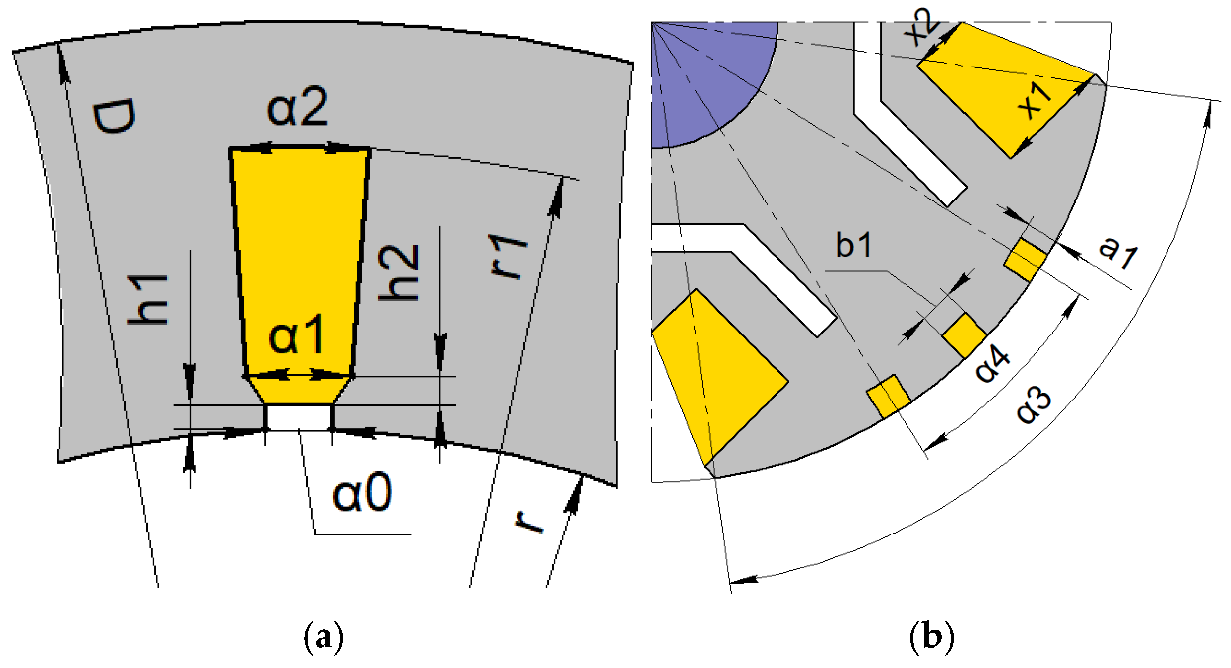
Basic-model parameter vector x consists of geometrical parameters, RMS values of the stator slot currents, phase angles of the stator slot currents, and the field winding sections’ currents.

Considering the symmetrical nature of the problem, the considered rotor positions lie within the range of 0–30 mechanical degrees. The total number of FE problems in this range is equal to 11. Linearized flux linkage dependencies on currents and rotor angular position are computed for all stator and rotor phases and normalized per one turn. Other quantities required for calculating losses [22] are also computed.

Stage 2. Then, the linearized dependencies found at the previous stage are used to compute HESM characteristics, taking into account PWM effects using a reduced-order model (ROM). The ROM is based on a system of ordinary differential equations. This model is explained in detail in [22]. The dependencies obtained in the previous stage can be easily recalculated for any number of turns. Losses in the transistors and diodes are not considered. Therefore, only the ratio of the numbers of turns of the harmonic and field windings, but not their absolute values, should be set. The reference number of field winding turns is assumed to be 100. It was assumed that the number of turns may take non-integer values. The turn numbers of the stator winding and of the field winding are positive. Negative values are allowed for the harmonic winding, which corresponds to reversing the connection direction of its phases, opposite to the initially chosen configuration.

The switching pulses of the power switches (gating signal) in the ROM-based simulation are formed as follows:

-

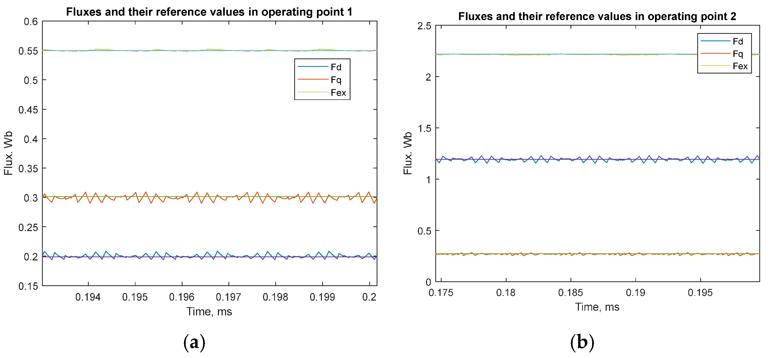
Proportional–integral (PI) controllers of stator magnetic flux dq-components are not simulated. Instead, the instantaneous phase fluxes Φ_ABC are assumed to be known (in a real system, they can be estimated, for example, using a flux observer). Since the currents in the windings are predetermined to simplify the calculations in the basic model, the dq-magnetic fluxes exhibit only minor oscillations around their mean values as the rotor rotates. It is assumed that the lookup table stores these mean flux values Φ_dq. Assuming constant rotor speed, the rotor position for the next PWM interrupt event is calculated. The flux values Φ_dq are then transformed into the inverter reference of the phase fluxes ${\mathsf{\Phi }}_{ABC}^{next}$. The corresponding phase voltage reference is then calculated through the following equation:

$$U_{ABC}^{ref}=f_{PWM}·\left({\mathsf{\Phi }}_{ABC}^{next}-{\mathsf{\Phi }}_{ABC}\right)+R{·I}_{ABC}$$

(1)

-

The phase voltage references $U_{ABC}^{ref}$ are transformed into the corresponding inverter output voltage by means of symmetrical space-vector PWM (SVPWM). It should be noted that this method directly controls the dq-components of the stator flux linkage, since the symmetrical SVPWM algorithm is insensitive to the zero-sequence component.

The excitation flux control algorithm (e.g., using an integral controller) is not considered in detail in this work. The duty cycle ratio of the injector switch VT7 (see Figure 2b) is assumed to be constant.

So, in addition to the dependencies obtained at the basic-model stage, ROM computation requires the vector of parameters y composed of the number of turns in the stator winding and in the harmonic winding phases, as well as the duty cycle ratios of the injector switch in both operating points.

To exclude transient processes from consideration and focus on steady-state values, the ROM simulation time is set to 0.2 s. The objective function values are evaluated over the last period of the ROM calculation. The computation of one operating point requires approximately 190 s using the basic model, followed by 12 s with the ROM. Since the evaluation of F(x) requires the calculation of the HESM characteristics at the two operating points listed in Table 2, this requires two basic model runs and also results in a total number of ROM runs of 2 × 45 = 90. Therefore, the computation time for F(x) is approximately 2 × 190 + 90 × 12 = 1460 s for the proposed model.

Since the HESM performance evaluation for two operating points takes about a week (168 h, 14,515,200 s) without using the reduced-order model [17], it can be said that the proposed approach speeds up the computations by four orders of magnitude.

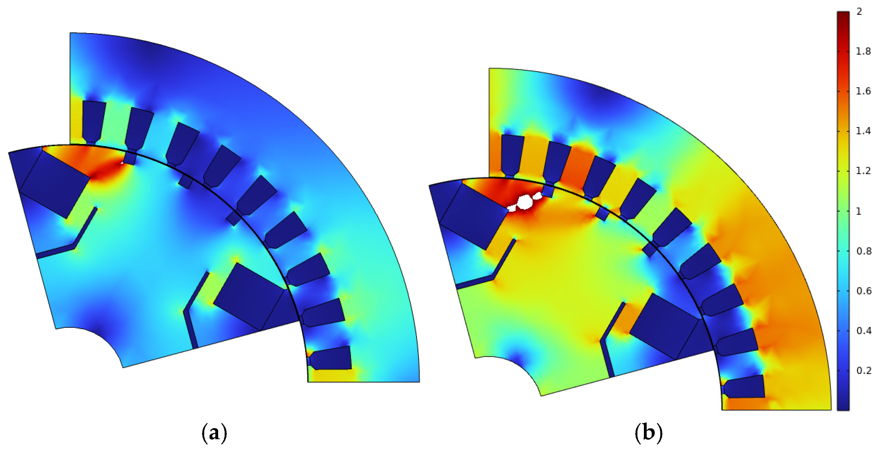
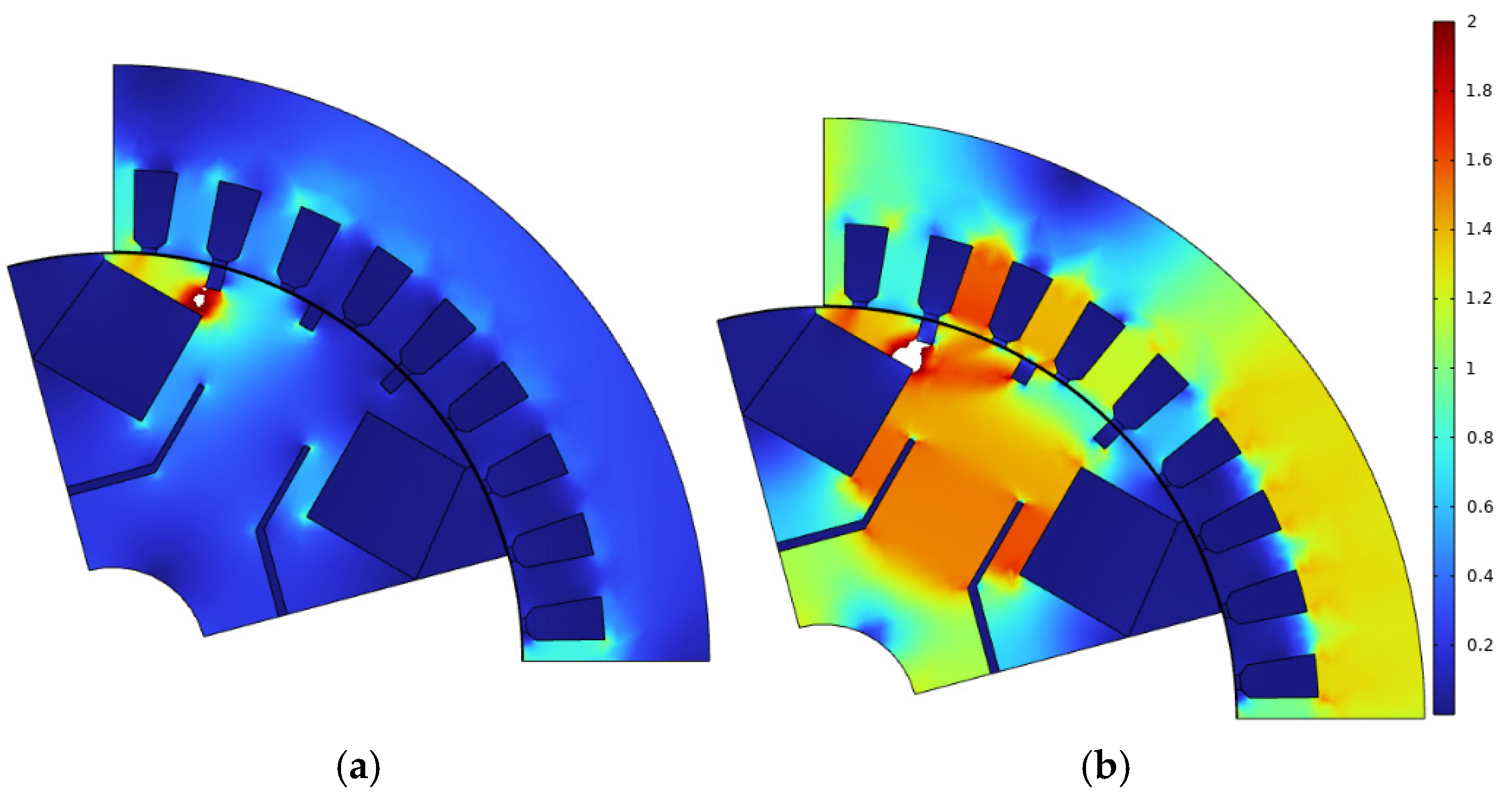
However, the ROM delivers correct results only if the considered motor working conditions are close to those in the basic model. Since the properties of magnetic circuits are defined mostly by the saturation level, a matching criterion is based on the comparison of the mean magnetic flux values. The values of the stator flux ${\Phi }_{dq}^{ROM}$ and ${\Phi }_{dq}^{base}$ can differ significantly in the case of overmodulation. The values of the excitation flux ${\Phi }_{ex}^{ROM}$ and ${\Phi }_{ex}^{base}$ can differ significantly due to an incorrect selection of the PWM duty cycle.

The measure of discrepancy between fluxes in the basic model and ROM $\epsilon$ is determined as follows:

$$\epsilon ={\displaystyle \frac{\left|{\Phi }_{dq}^{ROM}-{\Phi }_{dq}^{base}\right|}{\left|{\Phi }_{dq}^{base}\right|}}+{\displaystyle \frac{\left|{\Phi }_{ex}^{ROM}-{\Phi }_{ex}^{base}\right|}{\left|{\Phi }_{ex}^{base}\right|}}$$

(2)

Thus, magnetic saturation causes nonlinearity in the motor properties. To improve the accuracy of the current–flux relationships in the linear approximation used by the ROM, the series expansion is applied in the vicinity of the closest sinusoidal current condition (the basic model). Saturation is determined by magnetic fluxes, while discrepancy ε is a measure of the closeness of magnetic fluxes in the basic model and the ROM.

During the modeling, any feedback loops that require controller parameter tuning are excluded. While such tuning is acceptable when simulating or developing a specific machine, it becomes impractical when optimizing, and plenty of machines must be modeled. The cost of such simplification is that vectors x and y are not independent: ROM provides a correct result only if saturation levels in the basic model and ROM are close, and $\epsilon$ is small. The optimization procedure to obtain the correct x, y pair is described in the next section.

Although the voltage drop across the controlled switches and diodes is not taken into account in this study for the sake of model simplicity, this is not a fundamental limitation of the proposed approach, and the drop across the switches and diodes can be taken into account if necessary.

3.2. Optimization Routine

The optimization objectives are set as follows:

-

Efficiency maximization through the minimization of the sum of squared efficiency residuals from unity, where Eff₁ and Eff₂ are the efficiency values at the operating points of the duty cycle (see Table 2):

$$F_{\mathit{e}\mathit{f}\mathit{f}}={(1-{\mathit{E}\mathit{f}\mathit{f}}_1)}^2+{(1-{\mathit{E}\mathit{f}\mathit{f}}_2)}^2$$

(3)

—

Stator current minimization for both operating points: F_I = I₁² + I₂²;

—

Torque ripple minimization for both operating points: F_TR = TR₁² + TR₂².

The use of squared terms in these criteria implies that achieving high performance at both operating points is important. If one operating point yields a poor value for a certain indicator, squaring amplifies the effect, even if the same indicator is acceptable at the other operating point. Thus, if an indicator degrades at one operating point, it must be improved at that point, while improving it at the other operating point is of limited relevance.

Also, the following penalties are included in the objective function:

—

In order for the simulation to be correct and for x, y to correspond to each other, ε₁ and ε₂ (for both operating points) must be minimized.

—

The mechanical power obtained from the basic model and from the ROM may differ. Therefore, the final power value becomes known only after both calculation stages are completed. The power deviation at the ROM stage was evaluated for each operating point, and if it falls below the target value of 1720 W for each operational point, a penalty is applied. This deviation is expressed as:

$${Err}_{\mathrm{1,2}}=\left\{\begin{array}{cc}\hfill {\displaystyle \frac{1720}{P_{mech\mathrm{1,2}}^{ROM}}},& P_{mech}<1720W;\\ \hfill 1,& \hfill otherwise,\end{array}\right.$$

(4)

where indexes “1” and “2” correspond to the first and second operating points.

Due to the high computational complexity of even the proposed two-stage approach, the computationally efficient Nelder–Mead method is used in this study to speed up the calculations. An important advantage of the Nelder–Mead method over population-based or swarm-based methods often used for electrical machine optimization, such as the genetic algorithm, particle swarm algorithm, etc. [23,24,25,26], is the significant saving of computational time, which, without the use of supercomputers, allows for increasing the complexity of the mathematical model and number of optimization parameters, applying more complex optimization criteria, and also considering more than one operating point in the optimization process, which is particularly important for optimizing electrical machines that must provide a wide CPSR [4].

In this study, based on the optimization goals described above, the minimized objective function has the following form:

$$\mathit{F}(\mathrm{x},\mathrm{y})=\ln \left(F_{\mathit{e}\mathit{f}\mathit{f}}\right)+2·\left(\ln {\mathit{F}}_{\mathit{I}}\right)+0.5·\ln \left({\mathit{F}}_{\mathit{T}\mathit{R}}\right)+7.5·({\epsilon }_1+{\epsilon }_2+E_{rr1}+E_{rr2}),$$

(5)

where the values of F_eff, F_I and F_TR are given by Equation (3); the values of the flux linkage discrepancies between the ROM and the basic model ε₁ and ε₂ are given by Equation (2); the values of deviations in mechanical power based on the results of ROM calculations, compared to the basic model, Err₁ and Err₂ are given by Equation (4).

The first three terms in (5) correspond to the selected optimization goals: increasing efficiency, reducing the motor current drawn from the inverter, and reducing torque ripple. The natural logarithms of the F_eff, F_I and F_TR functions are calculated so that the optimization function considers relative, rather than absolute, reductions in these quantities with different units of measurement.

The weighting factors of 1, 2, and 0.5 reflect the relative priorities assigned to each optimization goal, based on the authors’ accumulated experience in designing comparable machines. The most important objective is to minimize F_I (factor 2), since reducing the consumed current allows for a reduction in the rating and cost of the inverter’s power semiconductor modules. The next most important objective is to increase efficiency (factor 1). Relatively less importance is assigned to the objective of reducing torque ripple (factor 0.5). A constant of 0.5 means that a 1% reduction in F_TR is equivalent in importance to a 0.5% reduction in F_eff. At the same time, a constant of 2 means that 0.5% reduction in F_I is just as important as a 1% reduction in F_eff.

The penalty sum (ε₁ + ε₂ + Err₁ + Err₂) can tend to zero, and the linear logarithm of such a value in this case will tend to infinity. Therefore, the logarithm for the last term in (5) is not calculated. The factor 7.5 is chosen to be large enough to ensure a gradual reduction in the deviations ε₁, ε₂, Err₁, and Err₂ to values acceptable for engineering calculations.

The function value depends on the basic model vector x and the inner optimization parameter vector y. The optimization procedure is based on the Nelder–Mead method and takes into account the fact that the computational time of the basic model and of the ROM differ by nearly a factor of ten.

Since ROM computation is computationally lean, the minimization of the objective function $F\left(x,y\right)$ can be performed rather fast by adjusting only the ROM parameter vector y:

$$F\left(x\right)=\underset{y}{\min }F(x,y).$$

(6)

This subroutine is called inner optimization. The minimum value of the objective function $F\left(x,y\right)$ can be found as the minimum of $F\left(x\right)$ by adjusting only vector x. This subroutine refers to outer optimization:

$$\underset{x,y}{\min }F\left(x,y\right)=\underset{x}{\min }F\left(x\right).$$

(7)

Since the proposed optimization routine is divided into outer and inner optimization subroutines, it can be called “two-level”. Thus, the algorithm for calculating F(x) and the optimal vector of the ROM parameter y^opt, which allows for achieving the minimum value of F(x,y) for given x vector, is designed as follows.

(1)

The basic model is computed at operating point 1 and linearized in its vicinity.

(2)

The basic model is computed at operating point 2 and linearized in its vicinity.

(3)

Optimization of the ROM parameters using the Nelder–Mead method. The termination criterion for the optimization is 45 function evaluations.

(4)

The minimum function value and the corresponding vector y^opt of the optimized ROM parameters are returned as a result.

Thus, evaluating $F\left(x\right)$ requires computing the HESM characteristics at the two operating points listed in Table 2 and, therefore, two basic model runs, which result in 2 × 45 = 90 ROM runs in total. The computation time for F(x) is approximately 2 × 190 + 90 × 12 = 1460 s.

The procedure described above is used as the objective function for the outer optimization. As a result, for each simplex vertex in the outer optimization, not only the value of F(x) is stored, but also the inner optimization parameters y^opt at which $\underset{y}{\min }F(x,y)$ is attained.

Let us consider the choice of the initial guess for the inner optimization parameters. During the first evaluation of F(x), the initial values for the inner optimization must ensure the absence of significant overmodulation of the stator winding voltage. In particular, the number of turns in the stator winding is deliberately chosen to be small. In subsequent evaluations of F(x), the initial inner optimization parameters should be selected as close as possible to the optimized values. Therefore, they are constructed from the optimized ROM parameter vectors $y_i^{opt}$, stored for each simplex vertex $x_i$ of the outer optimization:

$$y^{init}={\displaystyle \frac{\sum _i(F_{worst}-F(x_i\left)\right)y_i^{opt}}{\sum _i(F_{worst}-F(x_i\left)\right)}},$$

(8)

where $F_{worst}$ is the worst function value in the simplex, with summation carried out over all vertices of the outer optimization simplex.

In this way, the better vertices (with smaller objective function values) contribute more to the formation of the initial guess.

The restriction of the inner optimization to 45 function evaluations naturally reduces its accuracy. However, the algorithm develops as follows: initially, the outer optimization relies on approximate values of the objective function F(x_i) due to the limited accuracy of the inner optimization. As optimization proceeds, the initial values $y^{init}$ become increasingly close to the optimal ones, which in turn improves the performance of the inner optimization.

3.3. Optimization Parameters

Figure 3 depicts geometrical parameters listed in

Table 3. Predefined HESM Parameters.

Parameter	Value
Stack length, mm	125
Outer stator diameter D, mm	191
α0, mechanical degrees	2
h1, mm	0.8
h2, mm	1.6
Electric steel grade/thickness, mm	M270-50A/0.5 mm
Current angle at operating point 2, electrical degrees	90
α2/α1 ratio	1.14
Number of turns of the field winding	100

,

Table 4. Variable Parameters of the Outer Optimization Procedure.

Parameter	Initial Value	Optimized Value
Stator inner diameter 2∙r, mm	130	131.3
Stator slot bottom diameter 2∙r1, mm	154	157.6
α1, mechanical degrees	4.1	4.4
Air gap, mm	0.3	0.35
y1, mm	15	18.1
y2, mm	15	19.5
a1, mm	3	3.6
b1, mm	3	2.4
α4, mechanical degrees	30	28.5
RMS slot current at operating point 1, A	85.4	92.4
RMS slot current at operating point 2, A	90.0	97.7
Field winding section current (per coil) at operating point 1, A	375.7	327.1
Field winding section current (per coil) at operating point 2, A	412.5	437.0
Current angle at operating point 1, electrical degrees	160	150.17

and

Table 5. Variable Parameters of the Inner Optimization Procedure.

Parameter	Initial Value at First F(x) Call	Optimized Value at First F(x) Call	Initial Value at F(xopt) Call	Optimized Value at F(xopt) Call
Number of turns of phase a of the harmonic winding	4	3.77	7.37	7.50
Number of turns of phase b of the harmonic winding	6	5.59	9.60	9.22
Number of turns of the stator winding	14	18.27	34.83	34.69
PWM duty cycle ratio at operating point 1	0.2	0.195	0.0365	0.0374
PWM duty cycle ratio at operating point 2	0.25	0.204	0.0427	0.0432

. Table 3 contains fixed HESM parameters such as the main dimensions and some minor parameters of the slot-tooth zone (h1, h2, α2/α1 ratio), which do not significantly affect the HESM performance. Current advance angle at the base speed (operation point 2, Table 2) and high saturation taking place at this point is equal to 90 electrical degrees, because the field weakening is not required.

Table 4 shows initial and final values of the basic model parameters obtained by outer optimization. Table 5 consists of the initial and final values of the inner optimization vector at the first call of F(x) and at the end of outer optimization with optimal outer optimization parameter vector x^opt. Table 5 demonstrates that the discrepancy between the initial and final values of vector y reduces during the optimization process. Thus, the initial values vector $y^{init}$ approaches the optimal ones, making inner optimization more accurate.

4. Optimization Results

Table 6. HESM Performance Using the Basic Model.

Parameter	Before Optimization		After Optimization
Operating point	1	2	1	2
Speed, rpm	4200	1200	4200	1200
Supply frequency, Hz	140	40	140	40
Torque, N∙m	5.16	13.83	4.08	14.34
Mechanical power, W	2269.8	1738.4	1795.71	1802.39
Stator armature RMS current per slot, A	84.85	83.44	92.38	97.67
Field current per coil, A	373.32	382.32	327.13	436.95
Stator core loss, W	132.74	44.04	50.20	35.70
Rotor core loss, W	21.53	3.72	8.53	2.97
Armature copper loss, W	70.43	68.10	69.49	77.67
Field copper loss, W	57.73	60.55	23.08	41.19
Efficiency	0.889	0.908	0.92	0.92
Armature winding EMF per turn, V	12.78	7.44	6.50	6.31
Three-phase apparent power (without taking into account the power loss), V∙A	3254.0	1863.5	1800.54	1848.63
Power requirement, V∙A	3254.0	-	1848.63	-
Inverter utilization factor	0.53	-	0.97	-

and

Table 7. HESM Performance Using ROM.

Parameter	Before Optimization		After Optimization
Operating point number	1	2	1	2
Speed, rpm	4200	1200	4200	1200
Supply frequency, Hz	140	40	140	40
Torque, N∙m	3.91	13.83	3.91	13.71
Mechanical power, W	1720.6	1737.5	1717.90	1722.90
Stator armature current RMS, A	4.04	4.80	2.78	2.95
Stator core loss, W	158.5	58.1	56.60	44.77
Rotor core loss, W	29.9	10.2	10.01	5.99
Armature copper loss, W	54.1	76.5	75.98	85.25
Field copper loss, W	45.9	65.2	24.96	41.63
Rotor phase a copper loss, W	1.0	1.3	2.25	4.09
Rotor phase b copper loss, W	0.9	1.7	2.58	4.53
Total loss, W	290.2	213.0	172.38	186.25
Efficiency	0.856	0.891	0.909	0.902
Phase voltage RMS, V	230	230	230	230
Three-phase apparent power (without taking into account the power loss), V∙A	2785.2	3313.5	1921.4	2035.2
Power requirement, V∙A	3313.5	-	2035.2	-
Inverter utilization factor	0.52	-	0.84	-

show the results of HESM optimization at the final iteration and initial guess values. Table 6 shows the results obtained using the basic model. Table 7 consists of the results obtained using ROM and inner optimization. Figure 4 and Figure 5 demonstrate a flux density plot in the cross-section, computed using the basic model before and after optimization, respectively.

In Table 6, the inverter utilization factor is calculated as the minimum mechanical power divided by the power requirement (maximum three-phase apparent power) and reflects how well the HESM design performs in terms of minimizing the inverter rated current and inverter cost. The closer the inverter utilization factor is to one, the better.

Figure 6, Figure 7, Figure 8 and Figure 9 reveal the calculated waveforms using the ROM for the optimized HESM. Figure 6 shows the waveforms of the flux linkages in the last calculation period in comparison with their reference values. Only small deviations between the results obtained using the ROM and the reference values obtained using the basic model can be noticed. The flux linkage deviations from the basic model before optimization are ε₁ = 6.1% and ε₂ = 8.1% for operating points 1 and 2, respectively. After optimization, these deviations are reduced to ε₁ = 0.62% and ε₂ = 0.63%. This confirms the growing accuracy of the inner optimization due to the improvement of the initial guess value y^init during the outer optimization. Therefore, the deviation of the flux linkages from the basic model is minimized to a sufficient degree from a practical point of view.

Figure 7 and Figure 8 show the stator phase currents and field current, in comparison with their values obtained using the basic model. Flux linkages and currents oscillate in the vicinity of their reference values because of PWM effects. PWM-related oscillations are more pronounced in the field current.

As shown in Figure 9, the neutral current is predominantly positive. This indicates that the energy transferred when the injector switch is turned on almost entirely contributes to the excitation field creation and is absorbed by the motor. The energy returned through the freewheeling diode is negligible, which was also achieved during the optimization.

In Table 7, the inverter utilization factor is calculated as the minimum mechanical power divided by the power requirement (maximum three-phase apparent power) and reflects how well the HESM design performs in terms of minimizing the inverter rated current and inverter cost. The closer the inverter utilization factor is to one, the better.

As a result of the optimization, the parameters of the harmonic winding and field winding were adjusted. The mean field current at operating point 1 decreased and at operating point 2 increased. In the optimized design, the ratio of the mean field currents at point 2 to point 1 is 1.3357.

The maximum effective voltage per turn (operating point 1), according to the basic model, was reduced by approximately half: 12.783/6.4968 = 1.97. This allowed for an increase in the number of stator turns and a reduction in current.

After optimization, the air gap increased from 0.3 mm to 0.35 mm. On the one hand, increasing the air gap leads to an increase in the field current. On the other hand, it reduces the rotor saliency, which leads to improved machine performance at operating points in the field-weakening region. A slightly larger air gap reduced the braking effect of the reluctance torque characteristic of a WRSM.

Based on the optimization results for the HESM, taking into consideration PWM effects (Table 7), the following conclusions can be formulated:

(1)

Total losses at operating point 1 are reduced by a factor of 290/172 = 1.68; total losses at operating point 2 are reduced by a factor of 213/186 = 1.14, meaning that the efficiency is increased in both operating points.

(2)

Consequently, the efficiency at operating point 1 (maximum speed) increased from 85.6% to 90.9%, while at operating point 2 (base speed) it increased from 89.1% to 90.2%.

(3)

The required inverter power decreased by a factor of 3313/2025 = 1.63, and the inverter utilization factor increased significantly from 0.52 to 0.85. This enables the use of power switches for the HESM with substantially lower ratings and cost.

5. Conclusions

This paper proposes a novel computationally efficient optimization technique for a specific design of a harmonic-excited synchronous machine (HESM) supplied from a PWM inverter in a drive application with a constant power speed range of 1:3.5.

The distinctive feature of the proposed optimization technique is that it is based on a two-stage model including the basic FEM and ROM sub-models and considers the significant difference in their computational complexity to speed up the optimization process. The proposed approach allows for reducing the HESM optimization time by approximately four orders of magnitude, compared to the calculation using only FEA alone, as proposed in previous studies. This acceleration of calculations, in particular, allows us to take into account two operating points in the optimization process, namely, not only at the base speed, but also at the maximum speed in the field-weakening region.

During optimization, the efficiency increased by 5.3 percent points (pp.) at the maximum speed and by 1.1 pp. at the base speed. At the same time, the required inverter power was reduced by a factor of 1.63; therefore, the inverter utilization factor was significantly increased from 0.52 to 0.85. This makes inverter sizing easier and leads to lower drive system cost.