Article

Research on Deep Adaptive Clustering Method Based on Stacked Sparse Autoencoders for Concrete Truck Mixers Driving Conditions

1
Faculty of Intelligence Technology, Shanghai Institute of Technology, Shanghai 201418, China
2
College of Engineering, China Agricultural University, Beijing 100083, China
3
Fengzhi Ruilian Technologies Co., Ltd., Beijing 100096, China
*
Author to whom correspondence should be addressed.
World Electr. Veh. J. 2025, 16(10), 581; https://doi.org/10.3390/wevj16100581
Submission received: 18 July 2025 / Revised: 3 October 2025 / Accepted: 4 October 2025 / Published: 15 October 2025
(This article belongs to the Section Vehicle and Transportation Systems)

Abstract

Existing standard driving conditions fail to accurately characterize the complex characteristics of heavy-duty commercial vehicles such as concrete truck mixers (CTMs), while traditional dimensionality reduction methods have strong empirical dependence and an insufficient ability to capture nonlinear relationships. To address these issues, a novel method for constructing typical composite driving conditions that integrates deep feature learning and adaptive clustering is proposed. Firstly, a vehicle data monitoring system is used to collect real-world driving data, and a data processing and filtering criterion specific to CTMs is designed to provide effective input for feature extraction. Then, stacked sparse autoencoders (SSAE) are employed to extract deep features from normalized driving data. Finally, the K-means++ algorithm is improved using a nearest neighbor effective index minimization strategy to construct an adaptive driving condition clustering model. Validation results based on a real-world dataset of 8779 driving condition segments demonstrate that this method enables the precise extraction of complex driving condition features and optimal cluster partitioning. It provides a reliable basis for subsequent research on typical composite driving conditions construction and energy management strategies for heavy-duty commercial vehicles.

1. Introduction

Vehicle driving conditions serve as a key indicator of energy consumption sources in hybrid electric vehicles and a critical foundation for formulating energy management strategies. They reflect the real-time vehicle operation and road characteristics, typically described as the speed profiles and time distribution. Generally, driving conditions can be categorized into two types: one is standard-based driving conditions [1,2], and the other is real-world data-based driving conditions [3]. Given the complexity and diversity of real-world data, as well as the universality of standard-based driving conditions for hybrid power systems [4], the latter is more meaningful in theoretical research and engineering practice. However, most research on the design and performance of heavy-duty commercial vehicles is based on standard driving conditions [5,6,7].
In addition, for general-purpose vehicles with a single and stable energy consumption source, the energy demand is currently mostly characterized by driving cycles, given their uniform driving condition. However, for heavy-duty commercial vehicles such as concrete truck mixers (CTMs) or mining trucks with variable mass and multi-source characteristics [8,9,10], their driving conditions have composite attribute characteristics. The total power demand is not only related to driving conditions but also directly related to the real-time vehicle mass and the upper-part system speed. Tang et al. [11] gave the driving condition by collecting the mining truck operation data, including vehicle speed, vehicle mass and operation mode. To solve the problem, a vehicle real data experiment should be designed to construct the composite driving conditions.
Existing data-driven methods for constructing driving cycles can be primarily divided into three types: the micro-trip method [12], the Markov method [13], and the clustering method [14,15]. Topi J et al. [16] combined linear regression and neural networks to form a driving condition by randomly piecing together short trips. The micro-trip method demonstrates a prominent advantage in operational simplicity, yet its uncertainty leads to difficulty in defining a representative driving cycle [17]. Li et al. [18] determined the optimal number of clusters by combining multi-dimensional feature parameters and using cross-validation. Based on the Markov state transition matrix, the typical driving conditions for urban buses in Xi’an were constructed. Guo et al. [19] proposed an improved dual-chain Markov model based on the Markov chain and Monte Carlo theory combined with the self-organizing mapping neural network to synthesize the driving cycle. The Markov-based method relies on a state transition matrix calculated from the driving data, which may lead to deviations between the generated results and real driving characteristics [13]. Lin et al. [20] employed principal component analysis (PCA) and the K-means clustering algorithm to conduct feature dimensionality reduction and segment screening, and they then completed the synthesis of initial driving cycles via a random combination strategy. Subsequently, a hybrid-constrained autoencoder optimization model was used to minimize the mean error. The clustering method effectively ensures the diversity of driving cycles. However, determining the number of clusters remains a major challenge [21].
Typically, the extraction and compression of driving characteristic parameters are preprocessing steps for driving conditions construction. In Ref. [22], an analysis method of energy consumption characteristics was proposed, and the seven characteristic parameters of the driving conditions related to energy consumption characteristics were extracted from 30 parameters. Yang et al. [23] adopted a fuel consumption-oriented characteristic parameter selection method based on stepwise regression to improve the driving condition construction efficiency and effect. In Ref. [20], the principal components analysis (PCA) method was used to reduce the dimension of the initial characteristic parameters. Tong et al. [24] employed correlation analysis and the PCA method to perform dimensionality reduction on the characteristic parameters. Furthermore, the cargo mass was considered in the process of driving cycle construction for battery electric forklifts.
Currently, traditional PCA is mainly used to perform dimensionality reduction analysis on the original data [25]. While simple and efficient, this method may lose nonlinear correlation information in dimension-reduced data, resulting in inaccurate feature representation, which limits the effectiveness of subsequent clustering results. A stacked sparse autoencoder (SSAE), a deep neural network composed of multiple stacked autoencoders (AEs), can effectively fit complex data and capture nonlinear features [26,27,28]. Hence, this work proposes using SSAE to learn nonlinear features from a velocity profile varying with time, thereby enhancing the accuracy and reliability of clustering. Although it is widely used, the traditional K-means algorithm suffers from randomness in selecting initial cluster centers, and the choice of cluster number depends on practical scenarios [29,30,31], leading to unstable clustering performance.
Min et al. [32] proposed a 750 kV reactor voiceprint clustering method based on a deep adaptive K-means++ clustering algorithm (DAKCA), and the clustering effect had been improved. The key innovation was the integration of a Stacked Sparse Autoencoder (SSAE) into the clustering framework. It is demonstrated that the SSAE can effectively model complex, high-dimensional data by: (1) learning hierarchical nonlinear features through multi-layer sparse coding, avoiding the information loss of linear methods like PCA; and (2) using sparsity constraints to enhance the robustness of feature extraction. For our research on the CTMs, the driving data share two key characteristics with the reactor voiceprint data in Min’s study: high dimensionality and strong nonlinearity.
The SSAE algorithm they utilized could be adapted to extract nonlinear, time-varying features from the driving cycles of the CTMs. This adaptation directly addresses the first research gap highlighted in the Introduction, namely the limitations of traditional linear dimensionality reduction methods (such as PCA) in preserving nonlinear information from CTM driving data. However, this information is crucial for accurately representing the composite driving conditions. In addition, the deep adaptive clustering framework proposed in Min’s work, in which feature extraction and cluster center optimization are iteratively performed, is particularly crucial for solving the complex, multi-scenario-driven classification of the CTMs’ driving cycles in our research.
Therefore, inspired by Min’s research [32], we sought to adapt and extend the deep adaptive clustering framework, tailoring it to the unique features of CTM driving data to develop a more targeted and reliable clustering method specifically for CTM driving conditions. The main contributions can be summarized as follows.
(1)
The vehicle real data experiment considering the vehicle monitoring platform is designed to collect the driving data, including speed profiles, vehicle mass and operation mode sequences.
(2)
A deep adaptive clustering method based on the SSAE algorithm is utilized for the precise extraction of complex driving condition features and the achievement of optimal cluster partitioning.
The remainder of this paper is organized as follows. Section 2 presents the process of the SSAE-based feature extraction for the CTM. In Section 3, the adaptive cluster method is elaborated in detail. In Section 4, the results of the proposed deep adaptive clustering method are discussed. Conclusions are elaborated in Section 5.

2. SSAE-Based Feature Extraction

2.1. Data Collection Experiment

As shown in Figure 1, a vehicle data monitoring system is used to collect real-world driving data for a CTM with an agitation capacity of 8 m3. To avoid variability in driving styles from confounding the analysis of driving data clustering, this study employed a single driver during data collection to control for driving style as a variable, thus ensuring the collected data reflects the CTM’s real road conditions. Vehicle driving data are collected by accessing the vehicle’s OBD interface. Additionally, the built-in GPS module enables the acquisition of vehicle location, travel routes, and other vehicle information. The in-vehicle data terminal T-box transmits vehicle driving condition data and other information to the vehicle monitoring platform via communication networks.
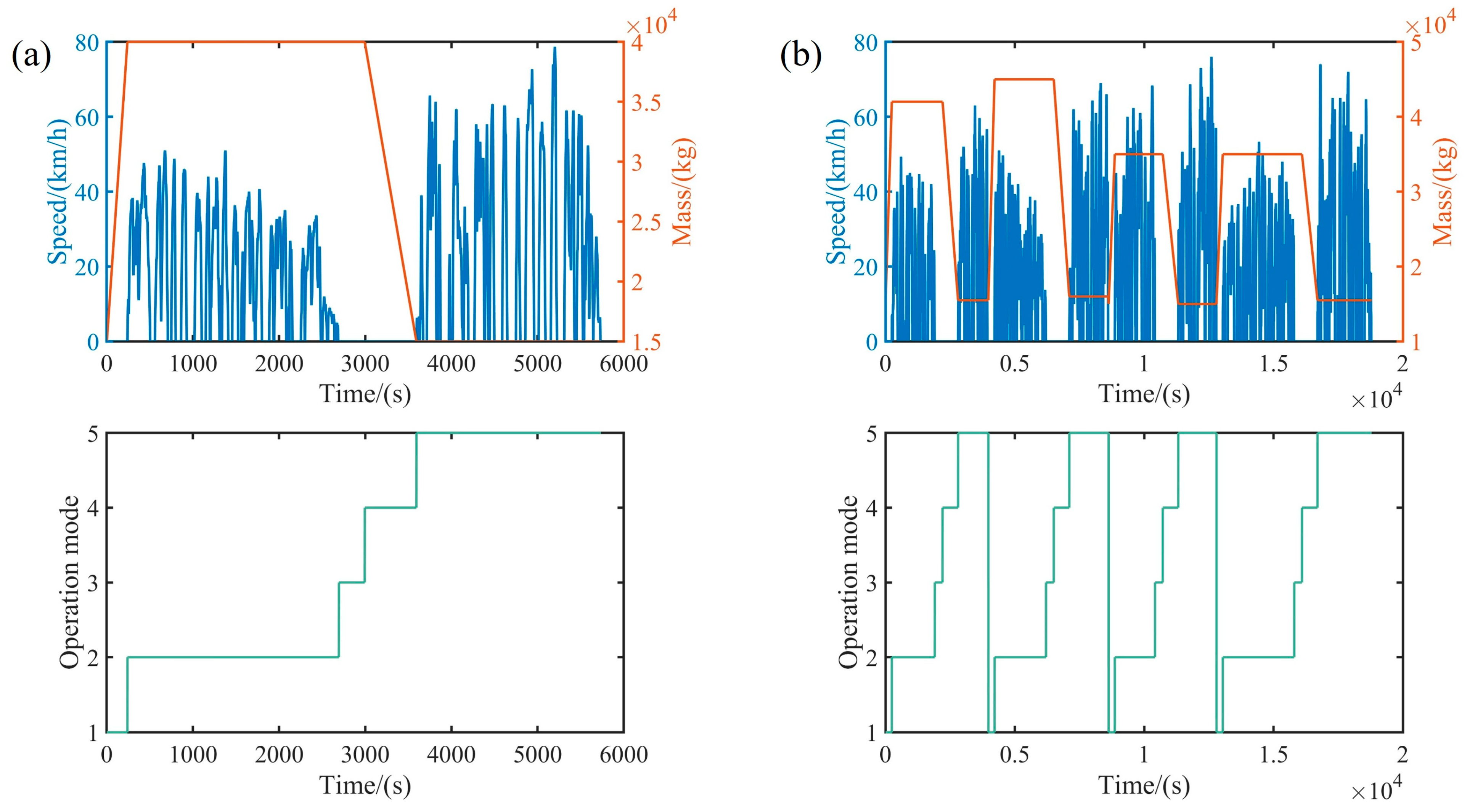
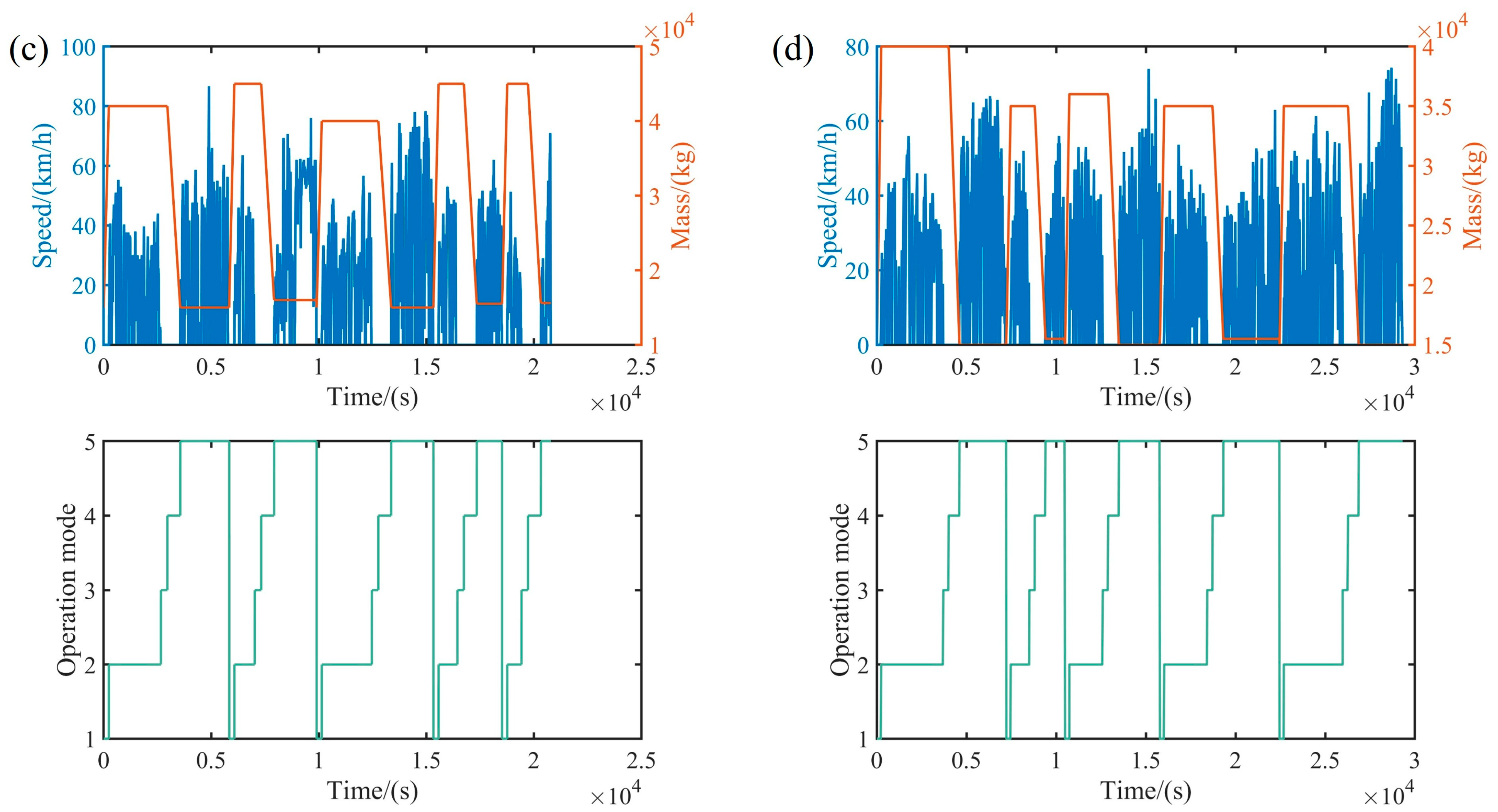
Based on the vehicle data monitoring system, the collected driving data consist of real-world driving records from a single driver at a concrete mixing plant near the Shanghai Outer Ring Road, China, over about two months. It can be divided into two phases: Phase 1 ran from 6 January to 1 February 2024, while Phase 2 covered 1 June to 30 June 2024. Figure 2a–d presents the partial collected driving data, including speed profiles, vehicle mass trajectories, and operation mode sequences. The operating modes of the CTMs can usually be divided into five types, namely loading, transporting, waiting, unloading, and returning, represented by numbers 1, 2, and up to 5, respectively. The above five operation modes are considered to form a working cycle of the CTMs.

2.2. Data Preprocessing

To ensure the reliability and applicability of the driving data used for subsequent research, it is necessary to preprocess the collected original driving data. Using the micro-trip partitioning method, the collected driving data of the CTM are divided into multiple micro-trips. Before this, it is necessary to convert the data directly obtained by the vehicle data monitoring system, as follows:
(1)
Since timestamps and corresponding trajectory points in the data file are in Greenwich Mean Time (GMT), they should be converted to Beijing time (GMT + 8);
(2)
The hexadecimal format of the ‘time’ keyword in the data file should be converted to a decimal time series and cross-day indexing appropriately processed.
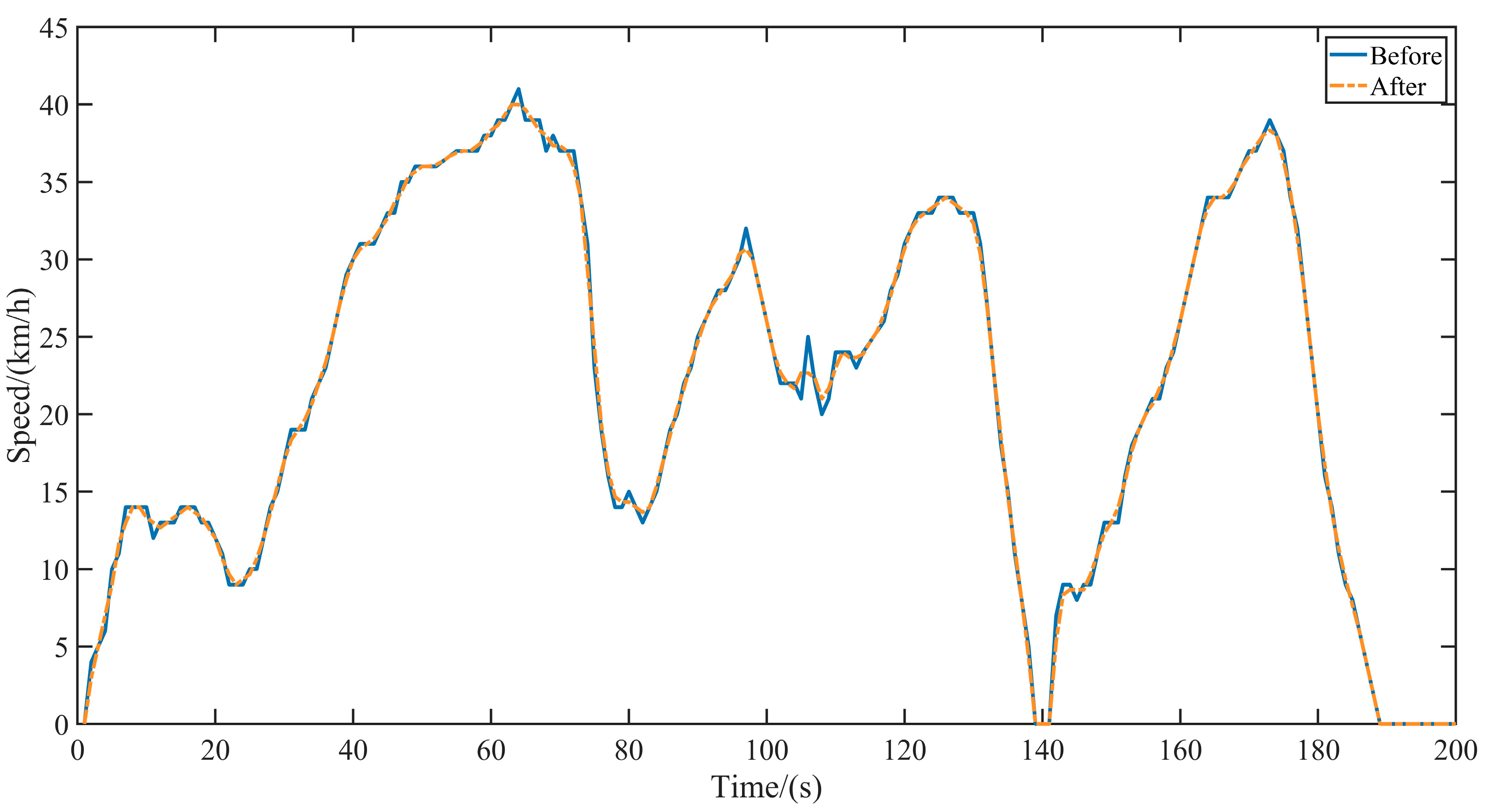
Subsequently, filtering is applied to each micro-trip, as shown in Figure 3. Based on the above, Figure 4 describes the flow chart of the driving data processing with main steps as follows.
(1)
Using the micro-trip partitioning method, the collected driving data of the CTM is divided into multiple micro-trips. After being chosen by criteria, a total of N m i c micro-trips are obtained. The following criteria are involved.
(a)
Due to equipment failures, abnormal driver operations, or weak GPS signals, some micro-trips have missing or discontinuous data. If a micro-trip has more than 10 consecutive missing sample points, it is discarded; otherwise, interpolation is used to supplement it.
(b)
According to relevant CTM standards, speed is limited to 50 km/h when fully loaded during transporting. However, no specific speed limit applies to empty returning.
(c)
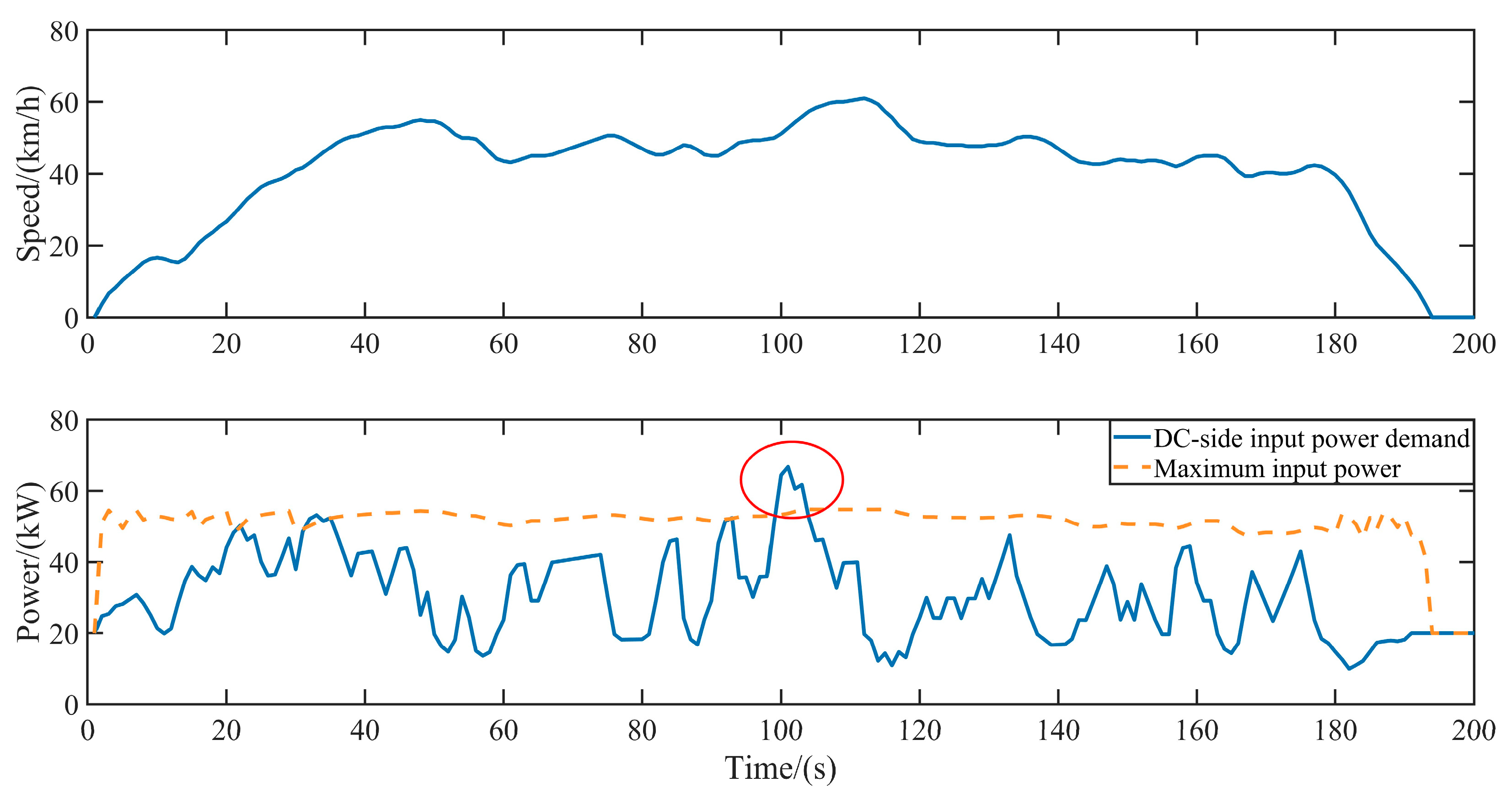
All micro-trips in the established database for CTMs should be validated against the studied powertrain. Thus, the DC-side power demand sequence of the drive motor controller for each micro-trip is calculated, discarding any micro-trip where power demand exceeds the drive motor’s external characteristic curve at any point.
Take the micro-trip shown in Figure 5 as an example. Between 99 and 104 s, the DC-side input power demand of the drive motor controller exceeds the maximum input power of the drive motor at the current rotational speed, indicating erroneous data. Thus, the micro-trip should be discarded.
(2)
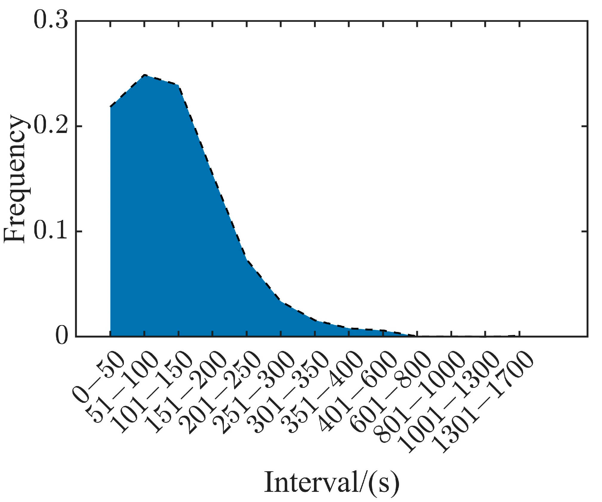
Due to the requirement of fixed input dimensions for SSAE, it is necessary to unify the duration of micro-trips. Divide the time interval and calculate the frequency distribution of the N m i c micro-trips, and select the average of the time interval with the highest frequency as time length T .
(3)
Cut or fill driving data in each micro-trip according to the established division criteria: if the real-time length T r of the micro-trip is less than T , cut the micro-trip and divide it into multiple sub-segments with time length T ; otherwise, fill the micro-trip to time length T with the last speed. Additionally, it should be noted to delete all segments with zero values.
Repeat step 3 until all micro-trips are processed, and finally obtain N R valid segments. The corresponding results are described in detail in Section 4.

2.3. Deep Feature Extraction

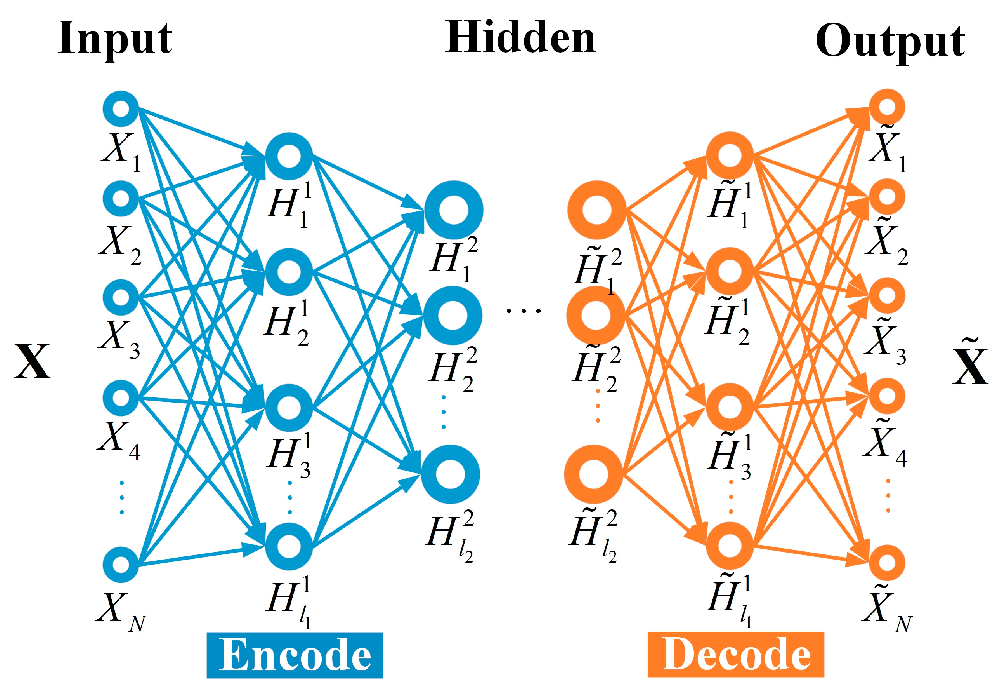
Autoencoders, as unsupervised learning algorithms, couple encoder and decoder structures to train feedforward neural networks via backpropagation, aiming to reconstruct input data for the effective extraction of data features [33]. Compared with standard autoencoders, a Sparse Autoencoder (SA) is an autoencoder subject to sparsity constraints on its hidden nodes, and it introduces the sparse penalty term [34]. To enable the deep mining of multi-scale data features, the Stacked Sparse Autoencoder with a deep neural architecture by the layer-wise stacking of sparse autoencoders is employed in the work.
Figure 6 depicts the structure diagram of the Stacked Sparse Autoencoder. The encoding process can be represented as:
H = f 1 W X + b
where X is the normalized input driving data; N is the dimension of input data; H and l m mean the hidden layer output and the number of neurons in the m -th layer, respectively; f 1 represents the encoding function; W and b are the weights and biases of the encoding layer, respectively.
The decoding process can be described as:
X ~ = f 2 W ~ H + b ~
where X ~ is the reconstruction value of the input data; f 2 represents the decode function; W ~ and b ~ are the weights and biases of the decoding layer, respectively. By continuously training and adjusting the weights and bias matrix, the loss function J S S A E W , b is minimized. The loss function is expressed as:
J S S A E W , b = 1 M i = 1 M L X i X ~ i +   β j = 1 l m K L ρ ρ j ~
where the first term is the total square error between input and output data and the second term is the sparse penalty term, represented by divergence K L ; M is the number of input samples; β is the weight of the sparse penalty term; ρ and ρ j ~ mean the sparsity factor and the activation level of the j -th hidden layer neuron, respectively; K L is represented as follows:
K L ρ ρ j ~ = ρ log ρ ρ j ~ + 1 ρ log 1 ρ 1 ρ j ~
Equation (3) converges to the desired local minimum, achieving deep feature extraction of driving condition data. The results are described in Section 4.

3. Deep Adaptive Clustering Method for CTMs Driving Conditions

3.1. Adaptive Cluster Method

Compared with the K-means algorithm, the K-means++ algorithm can better select the samples with larger dispersion as the initial clustering center, thus effectively avoiding the instability. However, it is difficult to preset the optimal number of clusters. Thus, an adaptive K-means++ method is employed in the work. By combining the clustering validation index based on nearest neighbors (CVNN) [32], select the number of clusters corresponding to its minimum value to determine the optimal number of clusters. Figure 7 gives the flow chart of the adaptive cluster method, and the cluster results are described in Section 4.
(1)
Input the feature samples extracted by the SSAE algorithm, and initialize parameters, mainly including the maximum allowable error ε and the range of the number of clusters K c K c m i n , K c m a x ,   K c m i n = 2 , where K c m a x takes the value of N R [35].
(2)
Randomly initialize the cluster center C . Then, update the cluster center C by calculating the centers and the mean of the samples’ features of each class.
(3)
Check whether the change in cluster centers before and after updating is less than ε . If it does, output the optimal number of clusters K c o p t , the corresponding CVNN under the optimal number, and the cluster labels; Otherwise, increase the number of clusters until the error condition is satisfied or the predefined maximum number of clusters is reached. The calculation method of the indicator CVNN is as follows,
C V K , m = S I C n K , m + C W C n K
where m is the number of neighboring points in the clustering process; S I C n K , m and C W C n K mean the normalized inter cluster separation and intra cluster compactness, respectively, which are calculated as,
S I C n K , m = S I C K , m max K c min K K c max S I C K , m C W C n K = C W C K max K c min K K c max C W C K
where S I C K , m and C W C K are the inter-cluster separation and intra-cluster compactness, respectively, whose calculation methods could refer to reference [32].

3.2. Fine Turning Process

The proposed deep adaptive clustering method for CTM driving conditions involves two-stage fine-tunings of SSAE: one during the SSAE-based deep feature extraction phase, optimizing parameters via supervised fine-tuning based on Equation (3); the other linked to the clustering process. In the clustering phase, to ensure the optimal result for the current cluster number K , the SSAE algorithm undergoes further fine-tuning once the CVNN value corresponding to K is obtained as described in Figure 7. Due to the lack of labels in driving data, fine-tuning in the first stage may fail to extract the most representative features, while fine-tuning in the second stage effectively addresses the problem [32]. Through the two-stage fine-tuning of the SSAE, the accuracy of the clustering results is ultimately improved.

4. Simulation Analysis

4.1. Data Collection and Preprocessing

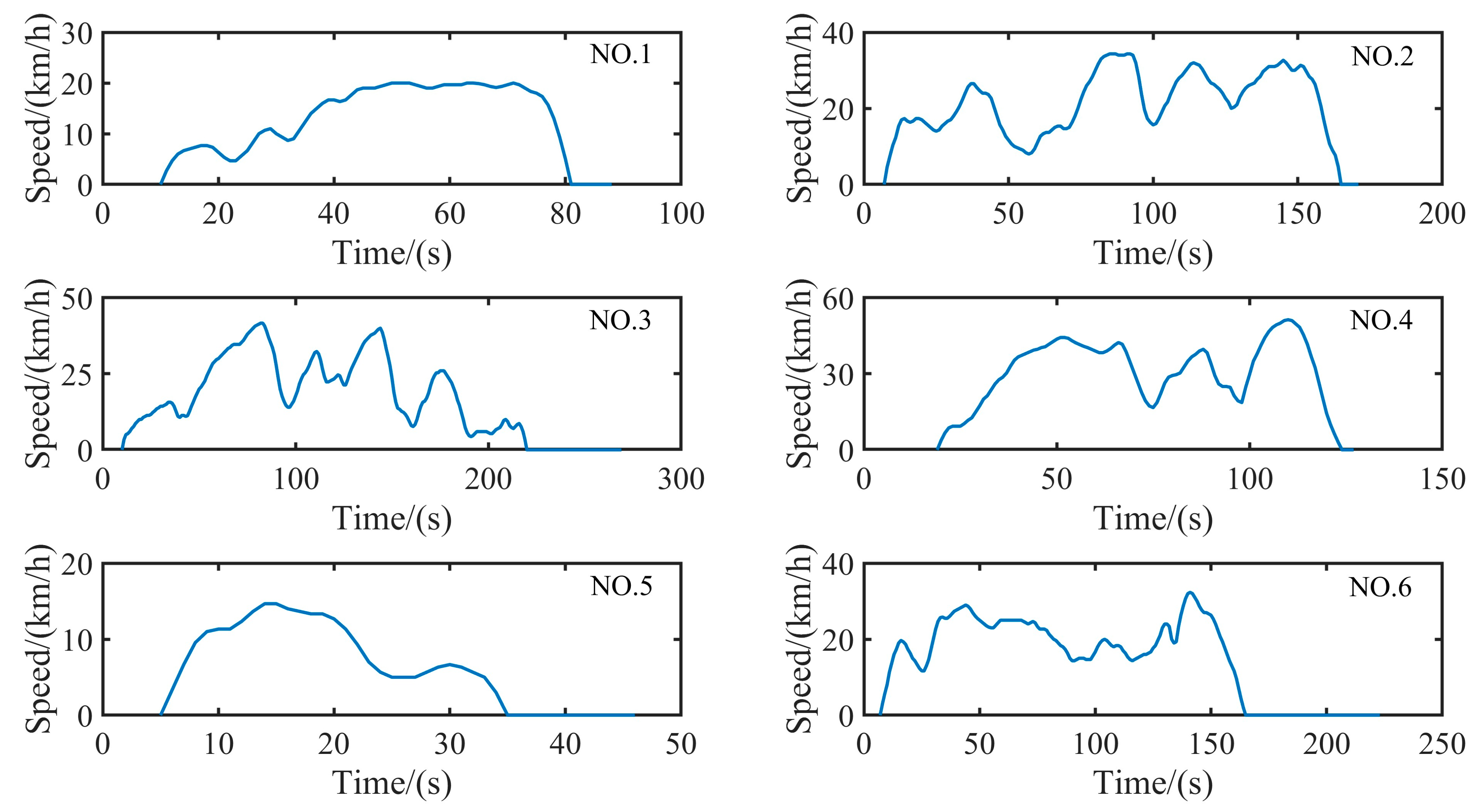
After driving data preprocessing, a total of N m i c = 5279 micro-trips are obtained, some of which are shown in Figure 8. Due to the requirement of fixed input dimensions for SSAE, it is necessary to unify the duration of micro-trips. Figure 9 gives the micro-trip frequency distribution diagram, and the figure indicates that micro-trip lengths most frequently lie in the 51–100 range. Hence, the time length T of the input data is selected to be 75.
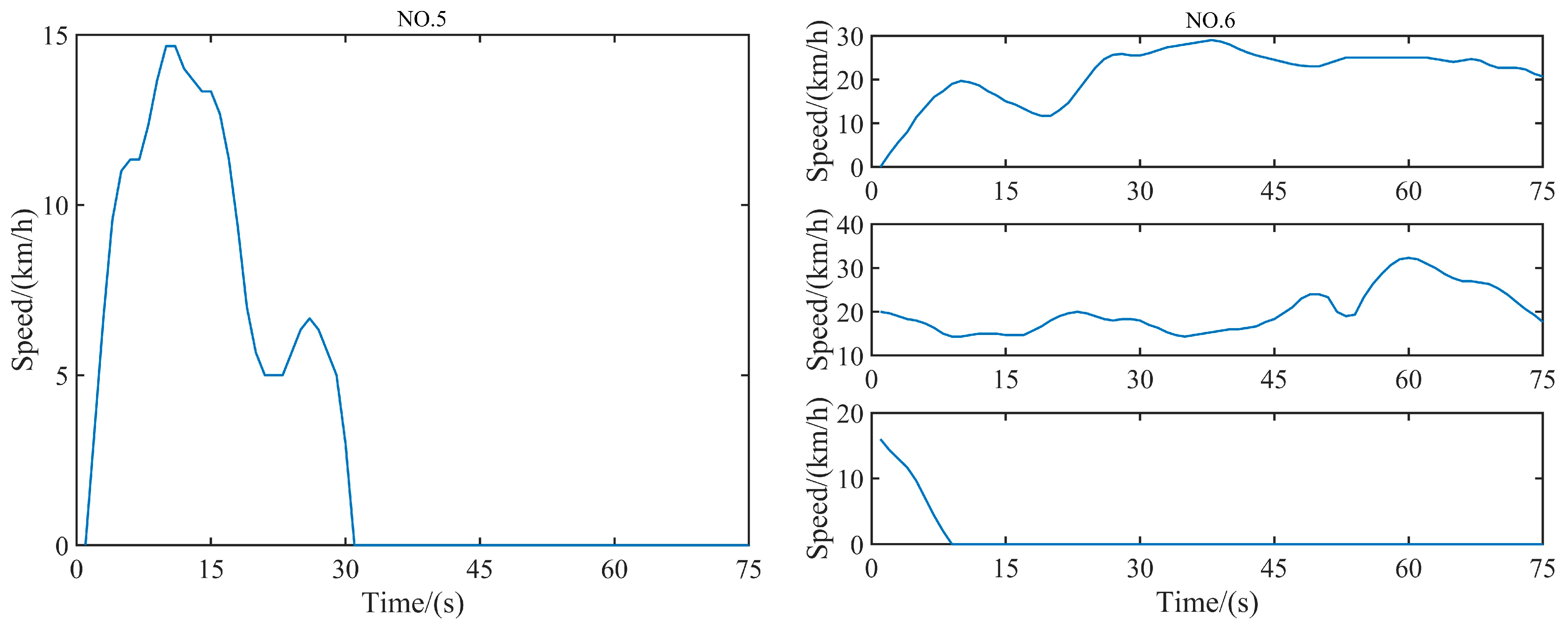
According to the designed micro-trips division criteria in Section 2.2, a total of N R = 8779 driving condition segments, each with a time length of T = 75, are obtained as input for the SSAE algorithm. The driving condition segments corresponding to the micro-trips shown in Figure 8 are depicted in Figure 10.

4.2. Feature Extraction Results Analysis

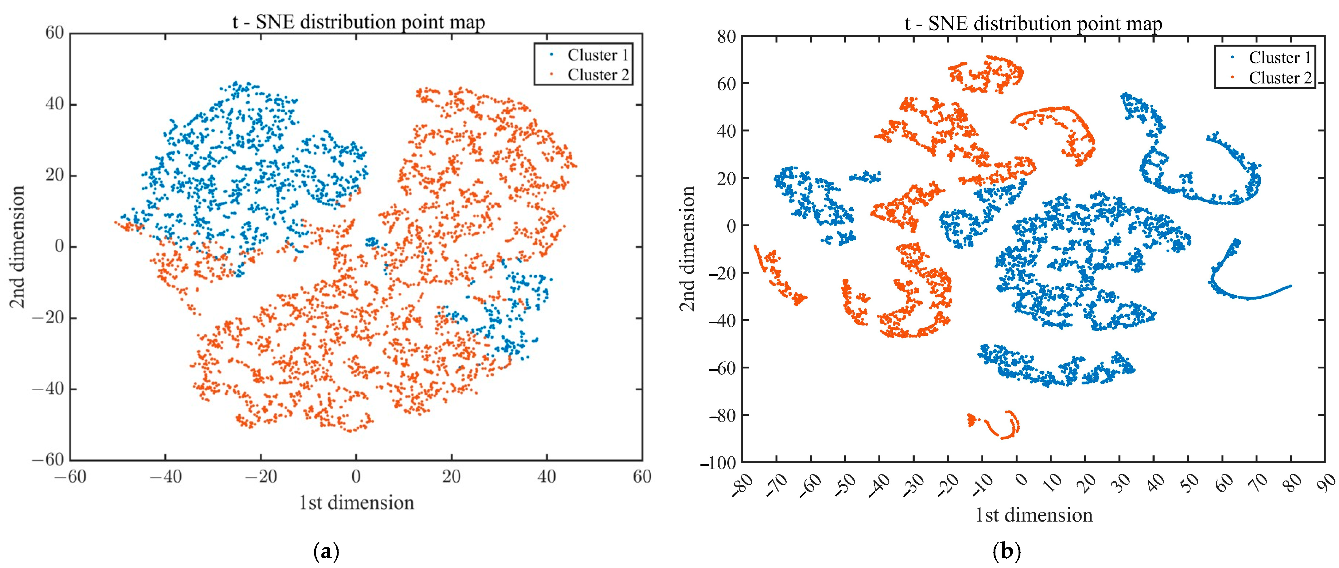
To verify the feature extraction capability of the SSAE algorithm, this section compares the performance of the SSAE and PCA algorithms. Figure 11a,b gives the two-dimensional t-SNE distribution point map of SSAE and PCA features, respectively. It can be seen that SSAE possesses the best feature extraction ability in driving condition data, completely separating different categories. By contrast, the PCA algorithm shows poor feature extraction performance, with some overlap between different categories in Figure 11a. The results indicate that using SSAE as the unsupervised feature extraction algorithm is effective. The reliance on experiential priors for feature selection, combined with limited nonlinear feature extraction capacity, significantly impairs PCA algorithm effectiveness.
To further validate the above conclusions, we use the criterion function A-index to evaluate the separability of features extracted by different methods, as shown in Equation (7).
S b S w = i = 1 K m i μ i μ f 2 i = 1 K f K i f μ i 2
where m i is the number of samples in class i ; μ i is the average eigenvector of the i t h class sample; μ f is the average eigenvector of total class samples, and it can be calculated as,
μ f = i = 1 K μ i K
The results in Table 1 show that the S b / S w index of SSAE is superior to other comparative algorithms, indicating that the features extracted by SSAE have the best separability.

4.3. Clustering Results Analysis

In this Section, a comparative analysis is conducted between the proposed deep adaptive K-means++ clustering method (DAKMC) and the baseline K-means++ clustering method. The baseline K-means++ approach described in the paper involves empirically selected operational features, PCA-based dimensionality reduction, and subsequent K-means++ clustering (EPKMC). The relevant network parameters for the proposed deep adaptive K-means++ clustering method are presented in Table 2.
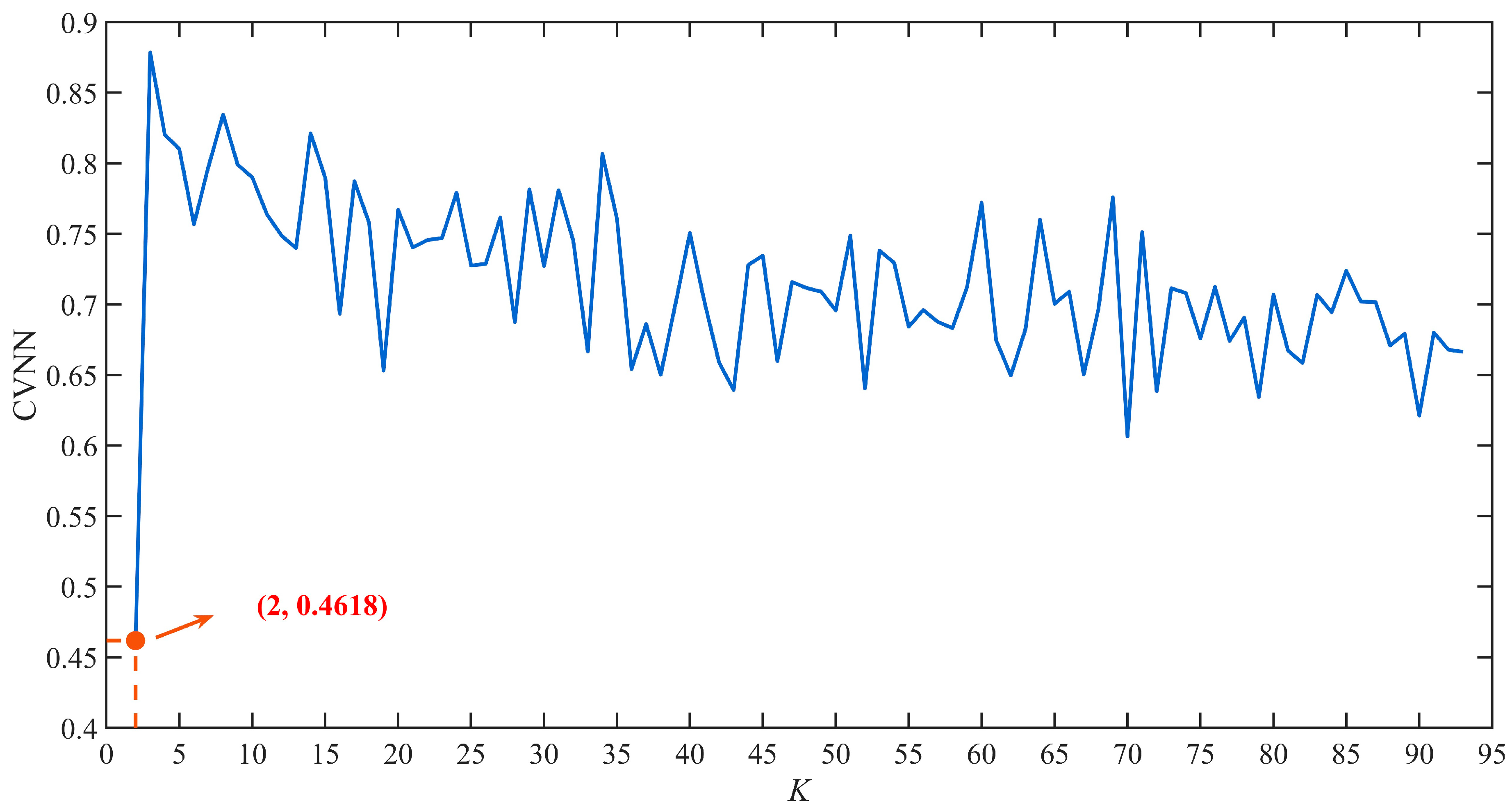
Figure 12 shows CVNN values for different numbers of clusters. The CVNN values vary with increasing K and reach their minimum at K = 2 . The minimum CVNN value accurately indicates the optimal cluster number, which ensures clear separation.
In addition, quantitative analysis of clustering performance across multiple indicators, including the Davies–Bouldin Index (DB), the Calinski–Harabasz Index (CH), and the Silhouette coefficient (SH) [36], is performed for both methods. The Davies–Bouldin Index (DB), Calinski–Harabasz Index (CH), and Silhouette coefficient (SH) can be calculated by Equations (9)–(11), respectively
s i = x i y i m a x y i , x i
D B I = 1 K i = 1 K R i . q t
C H = t r a c e B t r a c e W × N R K K 1
where x i , y i denote the shortest average distance from the i t h sample to all other points in each of the other clusters or the same cluster, respectively; t r a c e B and t r a c e W are the dispersion matrix of between-cluster B and the dispersion matrix of within-cluster W, respectively. The comparison results are presented in Table 3. Results show that the DB and SH values for the DAKMC method are lower and the DAKMC method achieves a CH index approximately 2× higher than the EPKMC method.
Notable differences exist in the performance of various clustering methods across different evaluation metrics. Specifically, the CH index relies on the ratio of between-cluster dispersion to within-cluster dispersion, the DB index focuses on measuring the balance between within-cluster compactness and inter-cluster distance, and the SH index is primarily used to assess the homogeneity of samples within clusters. The core design of the DAKMC method is centered on enhancing inter-cluster distinguishability, which directly amplifies the differences in CH values between the DAKMC method and other methods. However, the DAKMC method places limited focus on optimizing within-cluster compactness and sample homogeneity, which in turn leads to relatively small differences in DB and SH values across different methods. It is precisely due to the differences in sensitivity of various metrics to the design priorities of clustering methods that the performance of each clustering method varies across different metrics. However, the comparative analysis of the three indices reveals that the proposed deep adaptive K-means++ clustering method could achieve better clustering performance.
Based on the above analysis, it can be concluded that the proposed DAKMC method could accurately characterize the nonlinear relationship of the driving condition characteristics of the CTMs and thus obtain clustering results with better performance.

4.4. Future Research

The work aims to develop a deep adaptive clustering method for the driving cycles of concrete truck mixers. Simulations indicated that the method can extract deep features of driving cycles and accurately cluster the features of driving cycles. Compared with the traditional clustering algorithm, multiple evaluation indices are superior.
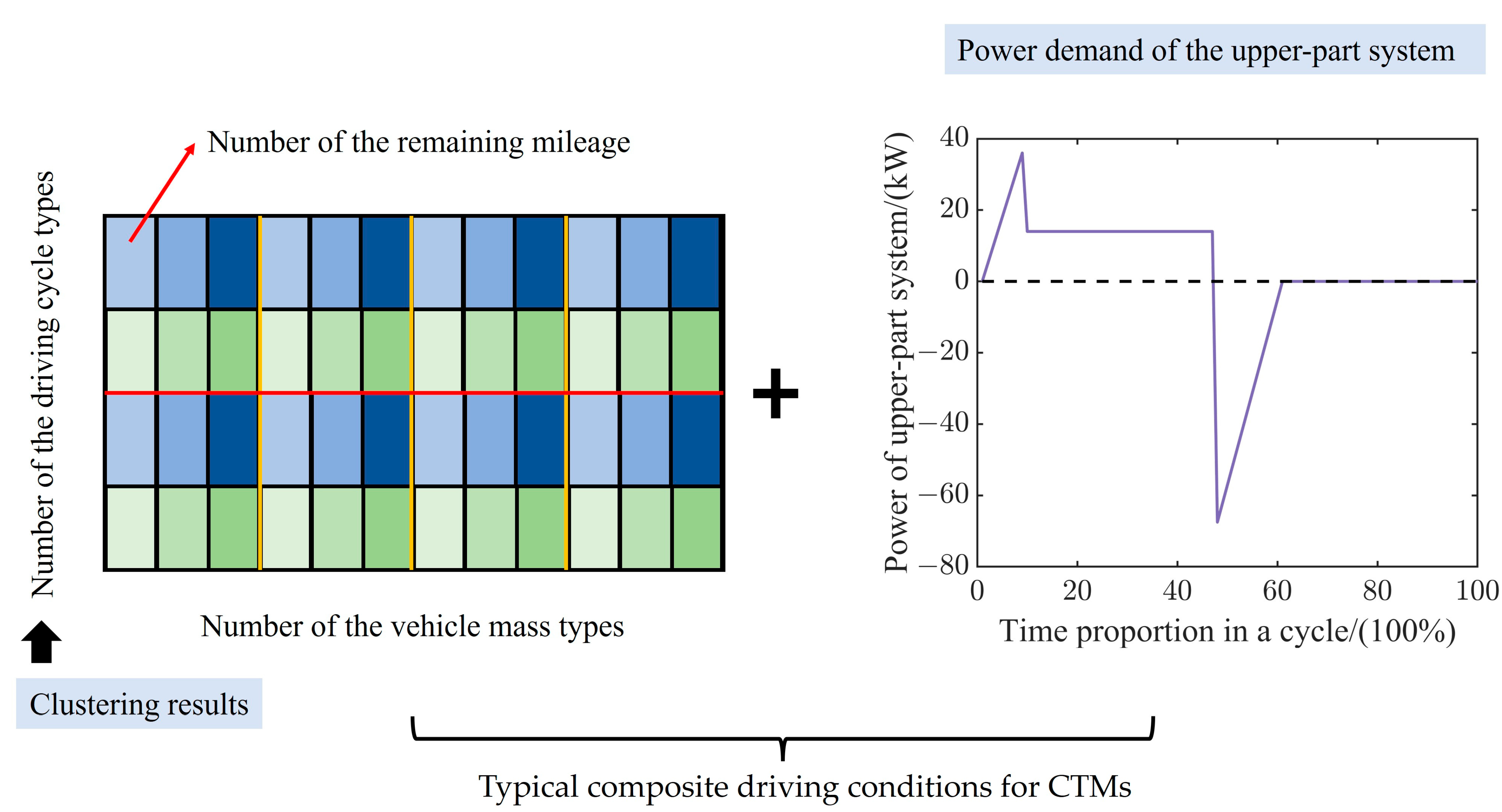
However, for the CTMs, their driving conditions have composite attribute characteristics. When constructing typical driving conditions for CTMs, except for the driving cycles, it is necessary to combine the operation modes, power demand of the upper-part system, vehicle mass, remaining mileage, and sampling time to build a typical composite driving condition. The schematic diagram of typical composite driving conditions is described in Figure 13. The operational conditions of the upper-part system are characterized by its power demand. A Shining View on-board recorder was used to collect the upperpart system’s operational conditions over one working cycle. As illustrated in Figure 13, the power demand of the upper-part system across a full working cycle is fitted, with the horizontal axis representing the time ratio of different operation modes.
As standard-based driving conditions miss CTMs’ unique traits, the composite driving conditions will resolve limitations in testing methodologies. Such specific cycles of the CTMs will act as standardized benchmarks, streamlining testing, shortening development timelines, and enabling Original Equipment Manufacturers (OEMs) to design user-aligned vehicles.

5. Conclusions

This paper aims to develop a deep adaptive clustering method for the driving conditions of concrete truck mixers. Given that current cloud platform technology enables the collection of large numbers of vehicle historical data, a vehicle data monitoring system and data processing criteria appropriate for CTMs’ characteristics are designed, ultimately resulting in an effective dataset with 8779 driving segments. To address the strong empirical dependency of traditional feature selection or dimensionality reduction, a stacked sparse autoencoder algorithm is applied to extract features and enhance the ability to capture nonlinear relationships. Finally, an adaptive K-means++ method is utilized to attain the clustering results. The method can extract deep features of driving conditions and accurately cluster the features of driving conditions. Compared with the traditional clustering algorithm, multiple evaluation indices are superior. Our research work will lay a foundation for the subsequent promotion of the construction of CTMs’ driving conditions and the in-depth research on energy management strategies.
For future research, further improvements could be made by integrating real-time data, including the operation modes, vehicle speed, vehicle mass, and driving data of the upper-part system, etc. Based on the proposed method, a composite real-world vehicle driving conditions will be built. This will enhance the control performance of the energy management strategies.

Author Contributions

Conceptualization, F.J. and H.X.; methodology, Y.H.; software, Y.H.; validation, F.J. and H.X.; formal analysis, H.X.; investigation, Y.H.; resources, F.J.; data curation, Y.H.; writing—original draft preparation, Y.H.; writing—review and editing, F.J.; project administration, H.X.; funding acquisition, F.J. All authors have read and agreed to the published version of the manuscript.

Funding

This research was funded by the National Key Research and Development Program of China (Grant No. 2022YFD2001204B) and the Research Start-up Fund for Talent Introduction of Shanghai Institute of Technology (Grant No. 101100250099088). In addition, the authors would like to acknowledge the support of the Fengzhi Ruilian Technologies Co., Ltd. of Beijing, China. The authors would like to thank them for their support and help.

Data Availability Statement

The raw data supporting the conclusions of this article will be made available by the authors on request.

Conflicts of Interest

Author Haiming Xie was employed by the company Fengzhi Ruilian Technologies Co., Ltd. The remaining authors declare that the research was conducted in the absence of any commercial or financial relationships that could be construed as a potential conflict of interest. The authors declare that this study received funding from Fengzhi Ruilian Technologies Co., Ltd. The funder was not involved in the study design, collection, analysis, interpretation of data, the writing of this article or the decision to submit it for publication.

Abbreviations

The following abbreviations are used in this manuscript:
CTMsConcrete truck mixers
SSAEStacked sparse autoencoders
PCAPrincipal component analysis
SAEStacked autoencoders
DBDavies–Bouldin index
CHCalinski–Harabasz index
SHSilhouette coefficient

References

  1. He, L.; Mo, H.; Wu, L.; Zhang, Y.; Tang, J.; Wu, H. Optimization on motor control strategy for a pure electric heavy truck with dual motor. J. Braz. Soc. Mech. Sci. Eng. 2025, 47, 530. [Google Scholar] [CrossRef]
  2. Liu, C.N.; Liu, Y. Energy Management Strategy for Plug-In Hybrid Electric Vehicles Based on Driving Condition Recognition: A Review. Electronics 2022, 11, 342. [Google Scholar] [CrossRef]
  3. Kemper, P.; Rehlaender, P.; Witkowski, U.; Schwung, A. Competitive Evaluation of Energy Management Strategies for Hybrid Electric Vehicle Based on Real World Driving. In Proceedings of the 2017 European Modelling Symposium (EMS), Manchester, UK, 20–21 November 2017; pp. 151–156. [Google Scholar]
  4. Liu, T.; Tan, W.; Tang, X.; Zhang, J.; Xing, Y.; Cao, D. Driving conditions-driven energy management strategies for hybrid electric vehicles: A review. Renew. Sustain. Energy Rev. 2021, 151, 111521. [Google Scholar] [CrossRef]
  5. Wu, H.S.; Li, L.; Wang, X.Y. A Combined Energy Management Strategy for Heavy-Duty Trucks Based on Global Traffic Information Optimization. Sustainability 2025, 17, 6361. [Google Scholar] [CrossRef]
  6. Chen, R.; Yang, C.; Wang, W.; Zha, M.; Du, X.; Wang, M. Efficient Adaptive Power Coordination Control for Heavy-Duty Series Hybrid Electric Vehicles with Model and Weight Transfer Awareness. IEEE Trans. Transp. Electrif. 2025, 11, 9404–9415. [Google Scholar] [CrossRef]
  7. Moghadasi, S.; Yasami, A.; Munshi, S.; McTaggart-Cowan, G.; Shahbakhti, M. Real-world steep drive cycles and gradeability performance analysis of hybrid electric and conventional class 8 regional-haul truck. Energy 2025, 320, 135128. [Google Scholar] [CrossRef]
  8. Huang, Y.; Wang, S.; Li, K.; Fan, Z.; Xie, H.; Jiang, F. Multi-parameter adaptive online energy management strategy for concrete truck mixers with a novel hybrid powertrain considering vehicle mass. Energy 2023, 277, 12770. [Google Scholar] [CrossRef]
  9. Huang, Y.; Jiang, F.C.; Xie, H.M. Adaptive hierarchical energy management design for a novel hybrid powertrain of concrete truck mixers. J. Power Sources 2021, 509, 230325. [Google Scholar] [CrossRef]
  10. Yan, Q.-D.; Chen, X.-Q.; Jian, H.-C.; Wei, W.; Wang, W.-D.; Wang, H. Design of a deep inference framework for required power forecasting and predictive control on a hybrid electric mining truck. Energy 2022, 238, 121960. [Google Scholar] [CrossRef]
  11. Tang, Q.; Hu, M.; Bian, Y.; Wang, Y.; Lei, Z.; Peng, X.; Li, K. Optimal energy efficiency control framework for distributed drive mining truck power system with hybrid energy storage: A vehicle-cloud integration approach. Appl. Energy 2024, 374, 123989. [Google Scholar] [CrossRef]
  12. Seunarine, M.B.; King, G. Representative Driving Cycles for Trinidad and Tobago with Slope Profiles for Electric Vehicles. Transp. Res. Rec. 2023, 2677, 1007–1016. [Google Scholar]
  13. Qiu, H.; Cui, S.; Wang, S.; Wang, Y.; Feng, M. A Clustering-Based Optimization Method for the Driving Cycle Construction: A Case Study in Fuzhou and Putian, China. IEEE Trans. Intell. Transp. Syst. 2022, 23, 18681–18694. [Google Scholar] [CrossRef]
  14. Wang, P.Y.; Pan, C.Y.; Sun, T.J. Control strategy optimization of plug-in hybrid electric vehicle based on driving data mining. Proc. Inst. Mech. Eng. Part D J. Automob. Eng. 2023, 237, 333–346. [Google Scholar] [CrossRef]
  15. He, H.; Guo, J.; Peng, J.; Tan, H.; Sun, C. Real-time global driving cycle construction and the application to economy driving pro system in plug-in hybrid electric vehicles. Energy 2018, 152, 95–107. [Google Scholar]
  16. Topi, J.; Kugor, B.; Deur, J. Neural network-based prediction of vehicle fuel consumption based on driving cycle data. Sustainability 2022, 14, 744. [Google Scholar] [CrossRef]
  17. Cui, Y.; Zou, F.; Xu, H.; Chen, Z.; Gong, K. A novel optimization-based method to develop representative driving cycle in various driving conditions. Energy 2022, 247, 123455. [Google Scholar] [CrossRef]
  18. Li, Y.; Liu, Y.; Shao, P.; Li, Z.; Song, W. Study on Components Durability Test Conditions Based on Combined Clustering and Markov Chain Method. Int. J. Automot. Technol. 2021, 22, 553–560. [Google Scholar] [CrossRef]
  19. Guo, J.; Xie, D.; Jiang, Y.; Li, Y. A novel construction and evaluation framework for driving cycle of electric vehicles based on energy consumption and emission analysis. Sustain. Cities Soc. 2024, 117, 105951. [Google Scholar] [CrossRef]
  20. Lin, J.X.; Liu, B.; Zhao, X.; Zhang, L. Intelligent Construction Method of Vehicle Condition Based on Hybrid Constrained Autoencoder. J. Transp. Syst. Eng. Inf. Technol. 2022, 22, 109–116. (In Chinese) [Google Scholar]
  21. Chen, Z.; Zhang, Q.; Lu, J.; Bi, J. Optimization-based method to develop practical driving cycle for application in electric vehicle power management: A case study in Shenyang, China. Energy 2019, 186, 115766.1–115766.13. [Google Scholar] [CrossRef]
  22. Wang, Y.; Li, K.; Zeng, X.; Gao, B.; Hong, J. Energy consumption characteristics based driving conditions construction and prediction for hybrid electric buses energy management. Energy 2022, 245, 123189. [Google Scholar] [CrossRef]
  23. Yang, D.; Liu, T.; Zhang, X.; Zeng, X.; Song, D. Construction of high-precision driving cycle based on Metropolis-Hastings sampling and genetic algorithm. Transp. Res. Part D Transp. Environ. 2023, 118, 103715. [Google Scholar] [CrossRef]
  24. Tong, Z.M.; Guan, S. Developing high-precision battery electric forklift driving cycle with variable cargo weight. Transp. Res. Part D Transp. Environ. 2024, 136, 104443. [Google Scholar] [CrossRef]
  25. Zhang, H.L.; Kong, D.; Yu, T.; Ao, G.; Shao, Y. Construction of urban driving cycle of light-duty vehicle based on LLEKM and Markov chain. J. Chang’an Univ. (Nat. Sci. Ed.) 2021, 41, 118–126. (In Chinese) [Google Scholar]
  26. Tufail, S.; Iqbal, H.; Tariq, M.; Sarwat, A.I. A Hybrid Machine Learning-Based Framework for Data Injection Attack Detection in Smart Grids Using PCA and Stacked Autoencoders. IEEE Access 2025, 13, 33783–33798. [Google Scholar] [CrossRef]
  27. Bi, J.; Guan, Z.; Yuan, H.; Yang, J.; Zhang, J. Network Anomaly Detection with Stacked Sparse Shrink Variational Autoencoders and Unbalanced XGBoost. IEEE Trans. Sustain. Comput. 2025, 10, 28–38. [Google Scholar] [CrossRef]
  28. Shi, C.; Luo, B.; He, S.; Li, K.; Liu, H.; Li, B. Tool Wear Prediction Via Multi-Dimensional Stacked Sparse Autoencoders with Feature Fusion. IEEE Trans. Ind. Inform. 2019, 16, 5150–5159. [Google Scholar] [CrossRef]
  29. Wang, B.L.; Tian, Y.; Yuan, J.K.; Wang, L.M.; Zhou, Y.C. Improvement method of semitrailer driving cycle construction based on clustering. J. Shandong Univ. Technol. (Nat. Sci. Ed.) 2023, 37, 26–33. (In Chinese) [Google Scholar]
  30. Zhu, D.; Xiao, B.; Xie, H.; Li, D.; He, H.; Zhai, W. Exploring trans-regional harvesting operation patterns based on multi-scale spatiotemporal partition using GNSS trajectory data. Int. J. Digit. Earth 2025, 18, 2466027. [Google Scholar] [CrossRef]
  31. Ggarwal, S.; Singh, P. Cuckoo, Bat and Krill Herd based k-means++ clustering algorithms. Clust. Comput. 2019, 22, 14169–14180. [Google Scholar] [CrossRef]
  32. Min, Y.Z.; Hao, D.Y.; Wang, G.; He, Y.; He, J. Reactor voiceprint clustering method based on deep adaptive K-means++ algorithm. Power Syst. Prot. Control 2025, 53, 1–3. (In Chinese) [Google Scholar]
  33. Mienye, I.D.; Sun, Y. Improved Heart Disease Prediction Using Particle Swarm Optimization Based Stacked Sparse Autoencoder. Electronics 2021, 10, 2347. [Google Scholar] [CrossRef]
  34. Wang, J.; Huang, Y.; Gao, X.; Wang, T.; Wang, X.; Hui, J. Blockage Location Algorithm of Multi-cylinder Fuel Injectors Based on Stacked Sparse Autoencoder. Acta Armamentarii 2024, 45, 3706–3717. (In Chinese) [Google Scholar]
  35. Lei, Y.; He, Z.; Zi, Y.; Chen, X. New clustering algorithm-based fault diagnosis using compensation distance evaluation technique. Mech. Syst. Signal Process. 2008, 22, 419–435. [Google Scholar] [CrossRef]
  36. Ahmed Al-Kerboly, D.M.; Al-Kerboly, D.Z.F. A Comparative Study of Clustering Algorithms for Profiling Researchers in Universities Through Google Scholar. In Proceedings of the 2024 IEEE 3rd International Conference on Computing and Machine Intelligence (ICMI), Mt Pleasant, MI, USA, 13–14 April 2024; pp. 1–5. [Google Scholar]
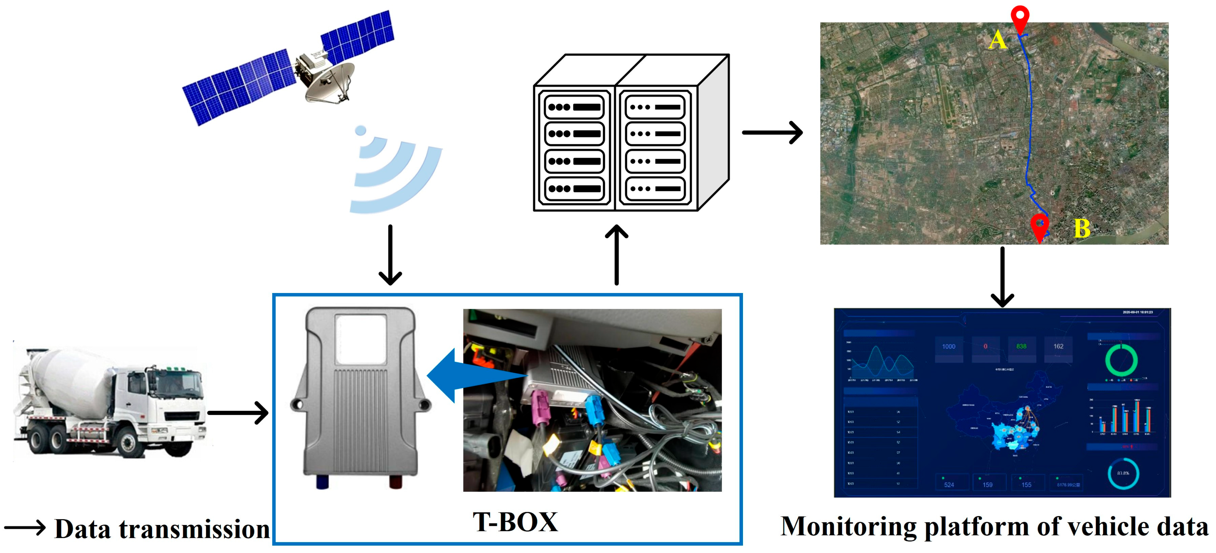
Figure 1. Vehicle data monitoring system.
Wevj 16 00581 g001
Figure 2. (ad) mean the collected driving data of the CTM (partial).
Wevj 16 00581 g002aWevj 16 00581 g002b
Figure 3. Diagram of initial driving data before and after filtering.
Wevj 16 00581 g003
Figure 4. The flow chart of the driving data processing.
Wevj 16 00581 g004
Figure 5. Diagram of micro-trips with excessive power.
Wevj 16 00581 g005
Figure 6. The structure diagram of the Stacked Sparse Autoencoder.
Wevj 16 00581 g006
Figure 7. The flow chart of the adaptive cluster method.
Wevj 16 00581 g007
Figure 8. Micro-trips (partial).
Wevj 16 00581 g008
Figure 9. The frequency distribution diagram of micro-trip time length.
Wevj 16 00581 g009
Figure 10. Unified length driving condition segments (partial).
Wevj 16 00581 g010aWevj 16 00581 g010b
Figure 11. Two-dimensional t-SNE distribution point map. (a) PCA features; (b) SSAE features.
Wevj 16 00581 g011
Figure 12. CVNN value variation with the cluster number.
Wevj 16 00581 g012
Figure 13. The schematic diagram of typical composite driving conditions for CTMs.
Wevj 16 00581 g013
Table 1. Comparison of S b / S w index.
AlgorithmValue
PCA0.41
Stacked AE1.03
Sparse AE0.44
SSAE2.10
Table 2. Network model parameters.
ParameterValueParameterValue
Hidden layers4Sparsity rate0.1
Nodes[70, 50, 40, 30]Weight attenuation parameter0.001
Sparse penalty term3Maximum cluster number K m a x = N R 93
Minimum cluster number K m i n 2
Table 3. Performance comparison of different clustering methods.
IndexEPKMCDAKMC
DB1.06200.9140
CH 3.7622 × 10 3 6.0452 × 10 3
SH0.59560.5562
Disclaimer/Publisher’s Note: The statements, opinions and data contained in all publications are solely those of the individual author(s) and contributor(s) and not of MDPI and/or the editor(s). MDPI and/or the editor(s) disclaim responsibility for any injury to people or property resulting from any ideas, methods, instructions or products referred to in the content.