Article

Improved MNet-Atten Electric Vehicle Charging Load Forecasting Based on Composite Decomposition and Evolutionary Predator–Prey and Strategy

1
School of Mechanical and Electronic Engineering, Shandong Vocational College of Light Industry, Zibo 255300, China
2
Transportation and Inspection Department, Shandong Deyou Electric Co., Ltd., Zibo 255000, China
3
Transportation and Inspection Department, Shandong Chenxiang Electric Equipment Co., Ltd., Zibo 255000, China
*
Author to whom correspondence should be addressed.
World Electr. Veh. J. 2025, 16(10), 564; https://doi.org/10.3390/wevj16100564
Submission received: 2 August 2025 / Revised: 18 September 2025 / Accepted: 23 September 2025 / Published: 2 October 2025
(This article belongs to the Section Charging Infrastructure and Grid Integration)

Abstract

In the context of low carbon, achieving accurate forecasting of electrical energy is critical for power management with the continuous development of power systems. For the sake of improving the performance of load forecasting, an improved MNet-Atten electric vehicle charging load forecasting based on composite decomposition and the evolutionary predator–prey and strategy model is proposed. In this light, through the data decomposition theory, each subsequence is processed using complementary ensemble empirical mode decomposition and filters out high-frequency white noise by using singular value decomposition based on matrix operation, which improves the anti-interference ability and computational efficiency of the model. In the model construction stage, the MNet-Atten prediction model is developed and constructed. The convolution module is used to mine the local dependencies of the sequences, and the long term and short-term features of the data are extracted through the loop and loop skip modules to improve the predictability of the data itself. Furthermore, the evolutionary predator and prey strategy is used to iteratively optimize the learning rate of the MNet-Atten for improving the forecasting performance and convergence speed of the model. The autoregressive module is used to enhance the ability of the neural network to identify linear features and improve the prediction performance of the model. Increasing temporal attention to give more weight to important features for global and local linkage capture. Additionally, the electric vehicle charging load data in a certain region, as an example, is verified, and the average value of 30 running times of the combined model proposed is 117.3231 s, and the correlation coefficient PCC of the CEEMD-SVD-EPPS-MNet-Atten model is closer to 1. Furthermore, the CEEMD-SVD-EPPS-MNet-Atten model has the lowest MAPE, RMSE, and PCC. The results show that the model in this paper can better extract the characteristics of the data, improve the modeling efficiency, and have a high data prediction accuracy.

Graphical Abstract

1. Introduction

Short-term power load forecasting is an important part of the efficient and economical operation of the power system and production scheduling. It is also an important means of achieving synergistic operation of the power system and balance between supply and demand [1]. However, with the establishment and development of the new power system, the new energy-led distributed energy, energy storage, and electric vehicles are connected to the power system on a large scale, which makes the power load present nonlinear and non-stationary characteristics and impacts the load prediction accuracy [2]. Therefore, it is necessary to explore and study the new power load forecasting method deeply, which provides an important guarantee for improving forecasting accuracy and the intelligent management level of a power system, realizing economic dispatching operations, energy savings, and emission reduction [3].
The main existing data forecasting algorithms in power systems are time series methods and artificial intelligence methods based on neural networks [4,5,6,7]. The typical representatives of time series methods are the Kalman filter method [8,9] and the regression model [10,11,12], which are more suitable for short-term forecasting of data. However, if the multivariate data fluctuate dramatically, are correlated, and have mutual perturbations, the use of such methods results in relatively large prediction errors. Therefore, time series methods cannot satisfy scenarios with high accuracy. The neural network algorithm has strong learning ability and adaptability and is widely used in related data prediction, especially in dealing with nonlinear problems and variable volatility. Nevertheless, it still faces the efficiency problem caused by training a large amount of historical data.
The single prediction algorithms commonly used today often fail to guarantee the precision and accuracy of the data when the time series is characterized by significant stochasticity, complexity, and non-linearity [13,14,15]. As a complement, a combined prediction model can fully exploit the advantages of a single model and improve the prediction performance through the combination of different models, signal decomposition, and parameter optimization [16]. Among them, the decomposition methods for nonlinear and non-stationary data series mainly include empirical modal decomposition (EMD) [17], variational modal decomposition (VMD) [18], and wavelet transform (WT) [19], as well as the corresponding improvement methods. The advantage of the EMD algorithm over algorithms such as VMD and WT is that there is no need to specify parameters artificially, and the data analysis process is adaptive. However, its disadvantage lies in modal aliasing, which has an impact on feature recognition and component prediction. Complementary ensemble empirical mode decomposition (CEEMD) reduces the residual auxiliary noise by adding paired Gaussian white noise, thus lessening the reconstruction error after decomposition [20,21]. In addition, the load data can be corrected and noise reduced using the singular value decomposition (SVD) algorithm to highlight the main features of the load data and eliminate the noise due to CEEMD decomposition or personal factors.
Conventional methods for data prediction, such as the autoregressive integrated moving average (ARIMA) [22], random walk (RW) [23], generalized autoregressive conditional heteroscedasticity (GARCH) [24], and vector autoregression (VAR) [25], demonstrate satisfactory performance in modeling linear relationships. However, they are unable to capture nonlinear patterns in data. To address this limitation, various nonlinear artificial intelligence and deep learning techniques—including artificial neural networks (ANNs) [26], support vector machines (SVMs) [27], and recurrent neural networks (RNNs)—have been developed for time series forecasting [28]. To overcome the issues of gradient explosion and vanishing gradients in standard RNNs, the long short-term memory (LSTM) architecture was introduced. LSTM utilizes gating mechanisms to selectively retain and integrate relevant information from historical data during training. Building on LSTM, the bidirectional LSTM (BiLSTM) incorporates two LSTM layers, enabling it to capture both forward and backward dependencies in sequences, making it particularly effective for time series forecasting [29]. Table 1 presents the previous literature on such technologies and their comparisons.
Different from many neural network models used in the past, short-term load prediction using a bidirectional recurrent neural network has the advantage of high accuracy but is prone to the problems of gradient vanishing and explosion. Short-term load prediction using bidirectional recurrent neural networks has the advantage of high accuracy but is prone to the problems of gradient vanishing and explosion. The problem of gradient vanishing is avoided by extracting the nonlinear coupling relationship through a convolutional neural network and building an enhanced recurrent neural network. By adding decomposition and error correction layers, the collected features are fed into the stacked bidirectional gated recurrent unit to reduce the errors in the prediction results, and better results are obtained [30]. On the downside, the structural parameters seriously affect the prediction accuracy of the network. If the network parameters are set improperly, the trained model cannot achieve the expected goal. Therefore, as an improvement, the evolutionary predator and prey strategy is used to optimize the learning rate in this paper [31]. Then, the multiple neural networks involving the convolutional neural network, bidirectional gated recurrent unit, and temporal pattern attention (MNet-Atten) are constructed, and an improved electric vehicle charging load forecasting model based on composite decomposition and evolutionary predator–prey and strategy is developed.
Given the discussed context, the contributions of this paper are threefold:
(1)
The load data are denoised by the composite decomposition algorithm to eliminate the pseudo components, which are based on the characteristics of electric vehicle charging load data. Meanwhile, the intrinsic mode functions and residual components with different amplitudes and frequencies are obtained.
(2)
The MNet-Atten prediction model is designed and implemented. The convolutional module is employed to capture local dependencies within the sequences, while recurrent and skip-connection modules are utilized to extract both long term and short-term temporal features, thereby enhancing the inherent predictability of the data.
(3)
By employing the EPPS algorithm, which possesses strong optimization capabilities and rapid convergence speed, to mine the intrinsic features of the MNet-Atten network, the learning rate is optimized and performs superposition calculations for load forecasting, thereby enhancing prediction accuracy.
The remainder of the paper is organized as follows. Section 2 gives the modeling of composite decomposition. Section 3 further proposes the modeling of the MNet-Atten Network. Section 4 develops the MNet-Atten based on the optimization of the evolutionary predator and prey strategy. In Section 5, model and case validation are shown to demonstrate the proposed method. Section 6 draws the conclusions.

2. Composite Decomposition

2.1. Singular Value Decomposition Model Based on Matrix Operations

This paper uses the SVD algorithm to correct and reduce the noise for the load data to highlight its main features and eliminate the noise caused by systematic or personal factors. The SVD algorithm can decompose the original load data signal into the superposition of several linear components, and the resulting singular values can reflect the different characteristics of the data [32].
For a real matrix A with rank r and order m × n, the following form can be obtained by singular value decomposition:
A = U Ξ V T = σ 1 u 1 v 1 + σ 1 u 1 v 1 + + σ r u r v r
where U U T = I and V V T = I , U and V are identity orthogonal matrix; Ξ is singular value matrix [32]; U R m × m , Ξ R m × n , V R n × n .
U = u 1 , , u i , , u m V = v 1 , , v i , , v m Ξ = d i a g σ 1 , , σ i , , σ m r = R a n k A < min m , n
where σ i fulfil the condition σ1σ2 ≥…≥ σm > 0, A T A v i = σ i v i .
The specific methods of noise reduction and data correction for SVD are shown below [32]:
Step 1: The data sequence Y y 1 , y 2 ,   , y N of the test is selected and the Hankel matrix K is constructed:
K = y 1 y 2 y n y 2 y 3 y n + 1 y N n + 1 y N n + 2 y N
Step 2: Assuming that the sequence of true values of the test data is Z and the noise sequence is H, the matrix K can be expressed as:
K = Z + H
Step 3: By performing singular value decomposition, the matrix A is decomposed into the following equation:
K = U z U h Z z 0 0 Z h V z V h T
where subscript z denotes the true sequence correlation matrix of the test data and subscript h denotes the correlation matrix of the noise sequence of the test data. In this paper, the SVD algorithm decomposition is used to find the singular values, and the singular values are eliminated to achieve the separation of noise.

2.2. Complementary Ensemble Empirical Mode Decomposition

The CEEMD is a method that can effectively deal with volatility, nonlinearity, and complex changing sequences and can adaptively decompose the data into multiple Intrinsic Mode Functions (IMFs) representing different local features of the original data according to the time series of the data.
For a given data x t , compute the maximum and minimum value points x max , t and x min , t . The mean value of the data time series is x ¯ t = x max , t + x min , t / 2 .
Then, s 1 , t 1 is taken as the initial data sequence, and the calculation is repeated m times until the average value tends to zero, and the screening threshold x b is applied as the judgment condition:
x b = t = 0 T s 1 , t m 1 s 1 , t m 2 s 1 , t n 1 2
Next, this paper defines the highest frequency sequence I M F 1 , t = s 1 , t 1 , s 1 , t 1 is the new sequence with the low frequencies removed, s 1 , t 1 = G t x ¯ t , and G t is the original sequence. Subtract I M F 1 , t from x t to obtain the remaining residuals sequence l 1 , t = x t a 1 , t . Repeat the above screening process continuously to obtain each IMF component and residual:
x t = i = 1 n I M F i , t + l n , t
In CEEMD, the reconstruction error after decomposition is significantly reduced by adding paired Gaussian white noise.
x i + t = x t + μ i + t x i t = x t + μ i t
where x i + t and x i t are the positive and negative sequences after adding random Gaussian white noise, respectively.
The final decomposition results of IMF components and residual components obtained by CEEMD decomposition of each positive and negative sequence are as follows:
I M F j = 1 2 n i = 1 n I M F i j + I I M F i j
l = 1 2 n i = 1 n l i + l i
The solution flow based on the CEEMD-SVD model is shown in Figure 1.

3. Modeling of MNet-Atten Network

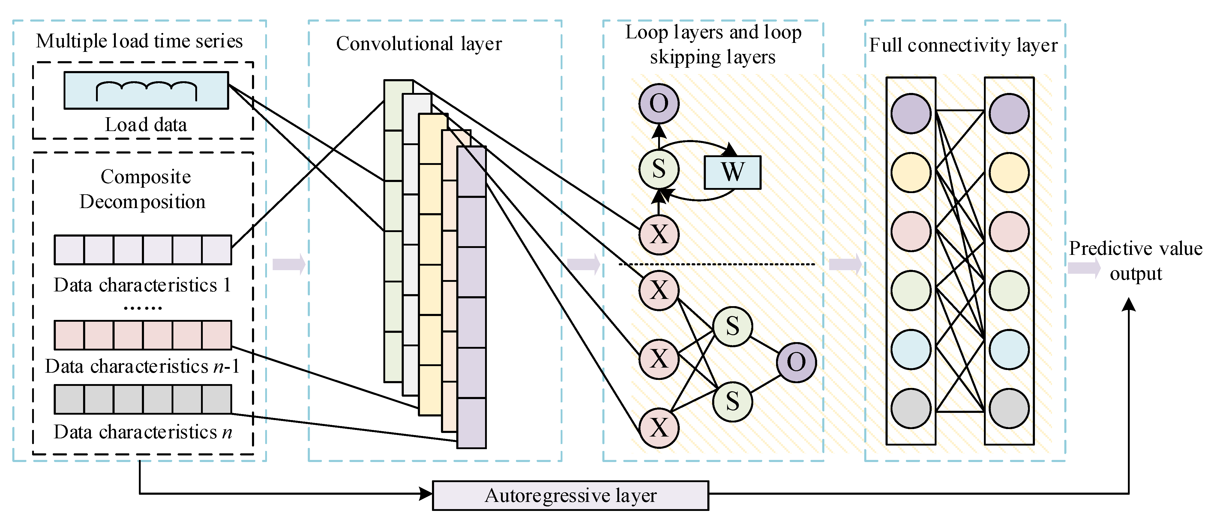
In this paper, the MNet-Atten prediction model is proposed to extract short-term and long term dependencies in the data through a nonlinear component consisting of convolutional, cyclic, and loop-skipping layers. The temporal pattern attention mechanism is used to focus on the key sequences and eliminate the disturbing factors. The linear features of the sequences are extracted by the autoregressive model, and the prediction results are obtained by superimposing the results of the nonlinear part and the linear part. The structure of the MNet-Atten network is shown in Figure 2.

3.1. Convolution Module

This module is a convolutional neural network without a pooling layer. It extracts the short-term local properties and dependencies between variables of the preprocessed time-series data and passes them to the loop and loop skip modules. The kth filter performs the convolution operation on the matrix Xt as shown in the following equation:
h k = R W k × X t + b k
where hk is the output feature vector, R denotes the activation function ReLU function, Wk represents the weight matrix of the convolution kernel connected to the kth feature map, Xt is the input vector of the convolution layer, and bk is the bias vector of this feature map.

3.2. Recurrent and Recurrent-Skip Module

The feature vectors output from the convolution module will be fed into the loop module and loop jump module at the same time. The BiGRU model consists of two layers of GRUs with the same output but in opposite directions of information transfer, which can receive information from both forward and reverse directions at any moment, overcoming the shortcomings of traditional GRUs in unidirectional information transfer, and can fully exploit the temporal characteristics of the load data to improve the data utilization rate and the accuracy of the model prediction. BiGRU is selected to form the loop module and loop skip module, and the basic structure of the BiGRU model is shown in Figure 3.
The hidden state of the loop module at time t is calculated as follows:
h t f = δ W f 1 x t + W f 2 h t 1 f
h t b = δ W b 1 x t + W b 2 h t + 1 b
h t = δ W 1 h t f + W 2 h t b
where xt is the input at time t, δ is the sigmoid activation function, h t f and h t b are the outputs of the positive-order GRU and negative-order hidden layer at time t, respectively, Wf1 and Wf2 are the weight vectors of the positive-order GRU hidden layer and the weight vector of the hidden layer at time t − 1, respectively, Wb1 and Wb2 are the weight vector of the hidden layer of the negative-order GRU model and the weight vector of the hidden layer at time t + 1, respectively, and W1 and W2 are the hidden layer weight vectors of the positive-order GRU model and the negative-order GRU model, respectively.
Long term temporal relationships between data can be captured by BiGRU’s bidirectional loop structure. For ultra-long term dependencies, BiGRU cannot extract effective features. To solve this problem, the loop-skipping module is introduced. The calculation process of the loop-skipping module is as follows:
h t f = δ W f 1 x t + W f 2 h t p f
h t b = δ W b 1 x t + W b 2 h t + p b
where p represents the number of cells to be skipped in the hidden layer, which is determined by the periodic law of the load sequence itself.
The output of the loop module at time t is h t R , and the output of the loop skip module from moment tp + 1 to t is h t S . The outputs of the loop and loop skip modules are combined via a full connectivity network, and the final result is used as a prediction for the nonlinear part. The full connectivity layer is calculated as follows.
h t D = W R h t R + i = 0 p 1 W i S h t i S + b
where h t D is the output of the nonlinear part at time t.

3.3. Modeling of Temporal Pattern Attention

In order to avoid ignoring the characteristics of important dimensional information in a time series, attention mechanisms have been proposed and widely used in the model prediction process. Classical attention mechanisms are based on the computation of correlation at a single time step, which makes it difficult to identify the information of a period that spans multiple time steps. The temporal pattern attention algorithm extracts features from the hidden state matrix by using a 1D convolutional neural network to extract the intrinsic links between the time series and different features, and the structure of the TPA algorithm is shown in Figure 4.
The input sequence is processed using BiGRU to obtain the hidden features htwht of the time series, w is the length of the time series. Define H = (htw, htw+1,…, ht−1} as the hidden feature, HC is the temporal pattern matrix extracted using one-dimensional convolution, and C denotes the filter. The computation and mapping process of the temporal pattern attention algorithm is as follows:
H i , j C = i = 0 p 1 H i , t w + l × C j , T w + l
f H i C , h t = H i C T W a h t
α i = δ f H i C , h t
y t 1 + Δ = W h W h W t + W v W t
where H i , j C is the eigenvalue extracted by the ith row vector through the jth filter of length T in Cj, T is the maximum length of the weights extracted by the filter, f is the evaluation function, αi is the attention weight, δ represents the sigmoid function, vt is the attention vector, yt−1+Δ is the final prediction result, Δ is the prediction time step, and Wa, W h , Wh, and Wv are the corresponding variables with different weight matrices for the corresponding variables, respectively.

3.4. Modeling of Autoregressive Module

Due to the nonlinear nature of the convolutional and recurrent modules, which affects the accuracy of the prediction model for input data that changes in a non-periodic manner, an autoregressive model is used as a prediction model for linear data in the load series. The prediction results can be calculated by the following equation:
h t L = k = 0 q a r 1 W k a r y t k + b a r
where W k a r and bar are the coefficients of the model, qar is the size of the input matrix, and h t L is the linear part of the prediction.
The final prediction result is weighted by the linear part of the output result h t L and the nonlinear part of the output result h t D :
Y ^ t = h t D + h t L
where Y ^ t is the final prediction at time t.

4. MNet-Atten Based on Optimization of Evolutionary Predator and Prey Strategy

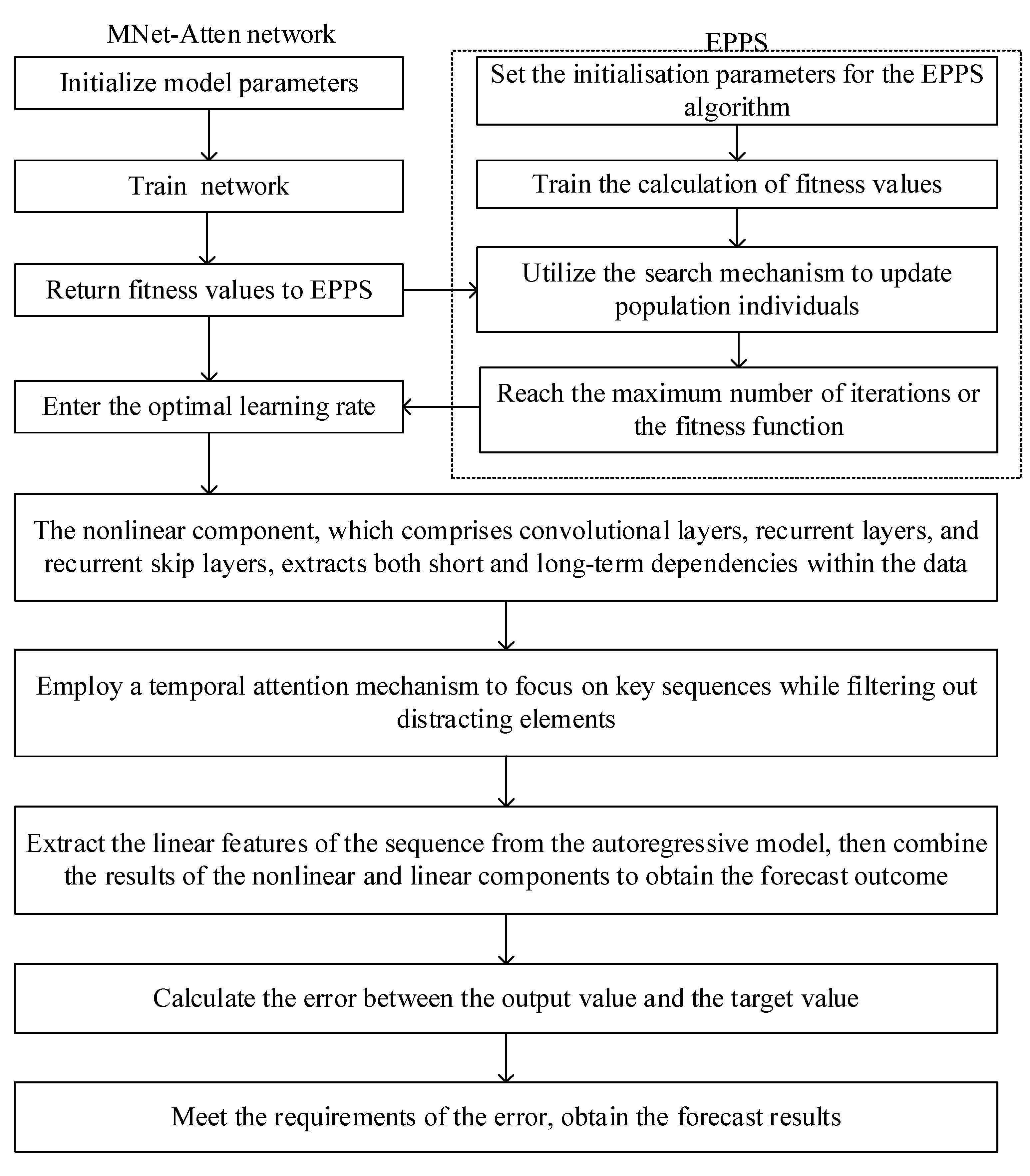
The intelligent optimization algorithm for evolutionary predation strategies EPPS is a population-based heuristic optimization algorithm that is learned and inspired by the group life behavior of animals. The EPPS algorithm is derived from the predation and escape behavior of hounds and goats and derives the hound predation mechanism, goat scanning mechanism, and goat escape mechanism. Further, four concepts of an empirical predator, strategic predator, prey, and safe position are proposed to model the predation-escape behavior between the two animals. Through the standard function test and the actual optimization problem, it has been confirmed that EPPS is superior to other evolutionary algorithms in terms of accuracy and stability [31]. The commonly used evolutionary algorithms include Group Search Optimizer (GSO), Set-Based Particle Swarm Optimization (SPSO), Differential Evolution (DE), and Covariance Matrix Adaptation Evolutionary Strategies (CMA-ESs). Therefore, this paper selects the EPPS algorithm to optimize the bidirectional long term and short-term memory network and achieve its optimal operation.
The exact procedure of the EPPS algorithm is shown below:
Step 1: Initialize the population size H o p , set the maximum number of iterations D m a x , and the strategic predator is 30% of the population size; calculate the population’s individual fitness value, and determine the prey and safe position.
Step 2: Calculate the scanning distance of the predator with the expression:
d = x c x g = i = 1 n x c i x g i 2
where x c and x g are the predator and safe position, respectively; x c i and x g i denote the ith predator and safe position, respectively.
Step 3: Execute the search mechanism of the prey; first scan the search at a zero angle, and then search right and left at a random angle:
x z = x c + d × L p ( φ )
x r = x c + d × L p φ + r 1 θ max / 2
x l = x c + d × L p φ r 1 θ max / 2
where φ R n 1 denotes a zero-degree viewing angle, L p ( φ ) is a unit vector, and r 1 R n 1 is a decimal uniformly distributed in (0, 1).
Step 4: Execute an empirical predator search mechanism:
x i = v + ψ K 0 , M , i = 1 , , ς
where v and M are the mean and covariance of all individuals that evolved, respectively; ψ denotes the step size; K 0 , M is a normal distribution with mean 0 and variance M; ς denotes the total number of empirical predators.
Step 5: Execute a strategic predator search mechanism. The strategic predator determines a predation path based on the direction and location of the prey’s escape:
x j = x c r 2 × x c x g , j = 1 , , ξ
Step 6: Calculate the fitness values of the individuals in the group and update the prey and safe position.
Step 7: Determine whether the iteration termination condition is reached. If yes, terminate the calculation; otherwise, repeat steps 2 to 6.
For the sake of clearly exhibiting the MNet-Atten network based on the optimization of the evolutionary predator and prey strategy, the flowchart and pseudocode are shown in Figure 5 and Table 2.

5. Model and Case Validation

In this paper, based on the changing characteristics of electric vehicle charging load data, the data are first processed using data decomposition algorithms based on CEEMD and SVD, and then the data prediction is completed by the MNet-Atten model optimized by the EPPS algorithm. The short-term electric vehicle charging load forecasting framework is shown in Figure 6.
The steps of the short-term electric vehicle charging load forecasting method based on EPPS- MNet-Atten with composite decomposition are as follows:
Step 1: The Hankel matrix is constructed, the diagonal matrix containing the eigenvalues is obtained by SVD decomposition, and data processing is performed to restore the data information by singular value inverse operation.
Step 2: The power load data are decomposed using the CEEMD model to obtain n intrinsic modal components I M F 1 , I M F 2 , , I M F n and the residual sequence ln.
Step 3: The power loads are divided into training and test sets in a particular proportion, and the MNet-Atten network is optimized using the EPPS algorithm to achieve MNet-Atten prediction based on the intrinsic modal components.
Step 4: The results of the n intrinsic modal components after MNet-Atten time series prediction are summed to obtain the load prediction value.
Step 5: Evaluation of algorithm performance: mean absolute percentage errors (MAPEs), root mean square error (RMSE), and Pearson correlation coefficient (PCC) are used as evaluation indexes for the prediction data. MAPE, RMSE, and PCC are calculated as follows:
P MAPE = 1 N t = 1 N Y t Y t Y t × 100 %
P RMSE = t = 1 N Y t Y t 2 / N
P PCC = t = 1 N Y t Y ¯ t Y t Y ¯ t i = 1 N Y t Y ¯ t 2 i = 1 N Y t Y ¯ t 2 × 100 %
where Y t and Y t denote the predicted and actual data at time t, respectively, Y ¯ t and Y ¯ t denote the mean of the predicted and actual data at time t, respectively, and N is the number of sample points on the prediction time scale.

5.1. Data Description and Data Pre-Processing

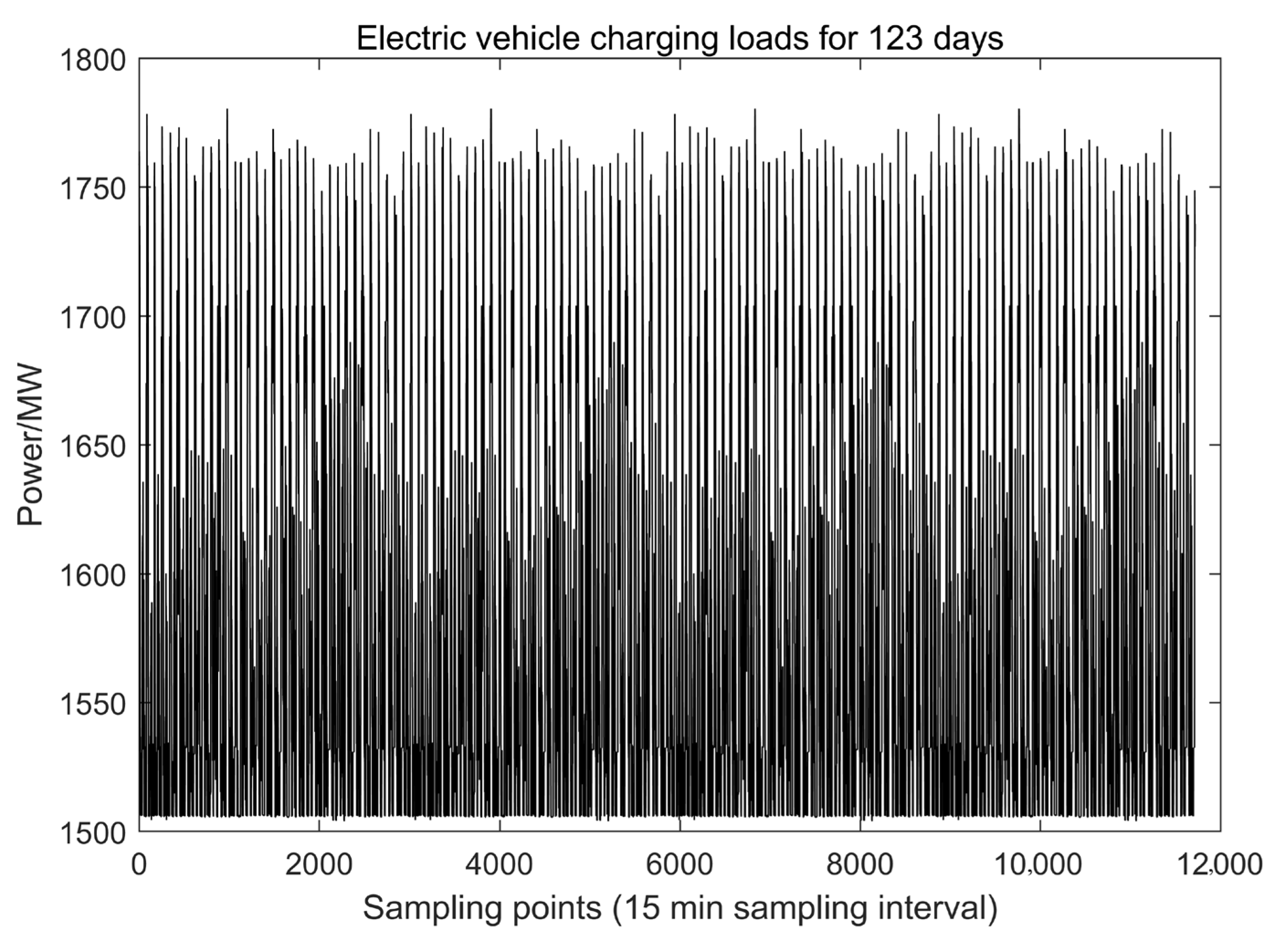
In this paper, the proposed model is implemented and solved using Gurobi (Gurobi Limited Liability Company, Beaverton, OR, USA) on a personal computer with an Intel Core i7-14650HX 5.20 GHz CPU and 32 GB of RAM. Furthermore, this paper implements MATLAB 2024b based on the Windows system to solve the improved MNet-Atten electric vehicle charging load forecasting. In addition, the electric load data from May to August 2024 at a charging station in Zibo City, Shandong Province, are used as a sample set, as shown in Figure 7. The sampling period is from 1 May to 31 August, with one sampling point data every 15 min interval and a total of 11,808 load data. The first 11,712 load data is the training set, and the last 96 load data is the test set. Meanwhile, the BiLSTM neural network uses the sigmoid function as the activation function of neurons. The output layer value is 1, the number of model layers is set to 3, and the number of neurons in the two layers is 60 and 40, respectively. The network training uses the Adam optimization algorithm.
The SVD has a noise reduction function, and the threshold for the cumulative percentage of singular values in this paper is 85% [33]. The values of any three consecutive days in the dataset are selected for singular value analysis. In this paper, a data sampling point is set every fifteen minutes, and the number of samples is ninety-six in total, with a total of two hundred and eighty-eight data sampling points accumulated in three days, and the comparison before and after noise reduction is shown in Figure 8. As can be seen from Figure 8 within the circle, the singular value decomposition based on matrix operation can, to a certain extent, reduce the noise of the original load data, eliminate the individual spikes that may be caused by the noise, and smooth the load curve, while preserving the original load cycle characteristics.

5.2. Data Decomposition Based on Composite Decomposition

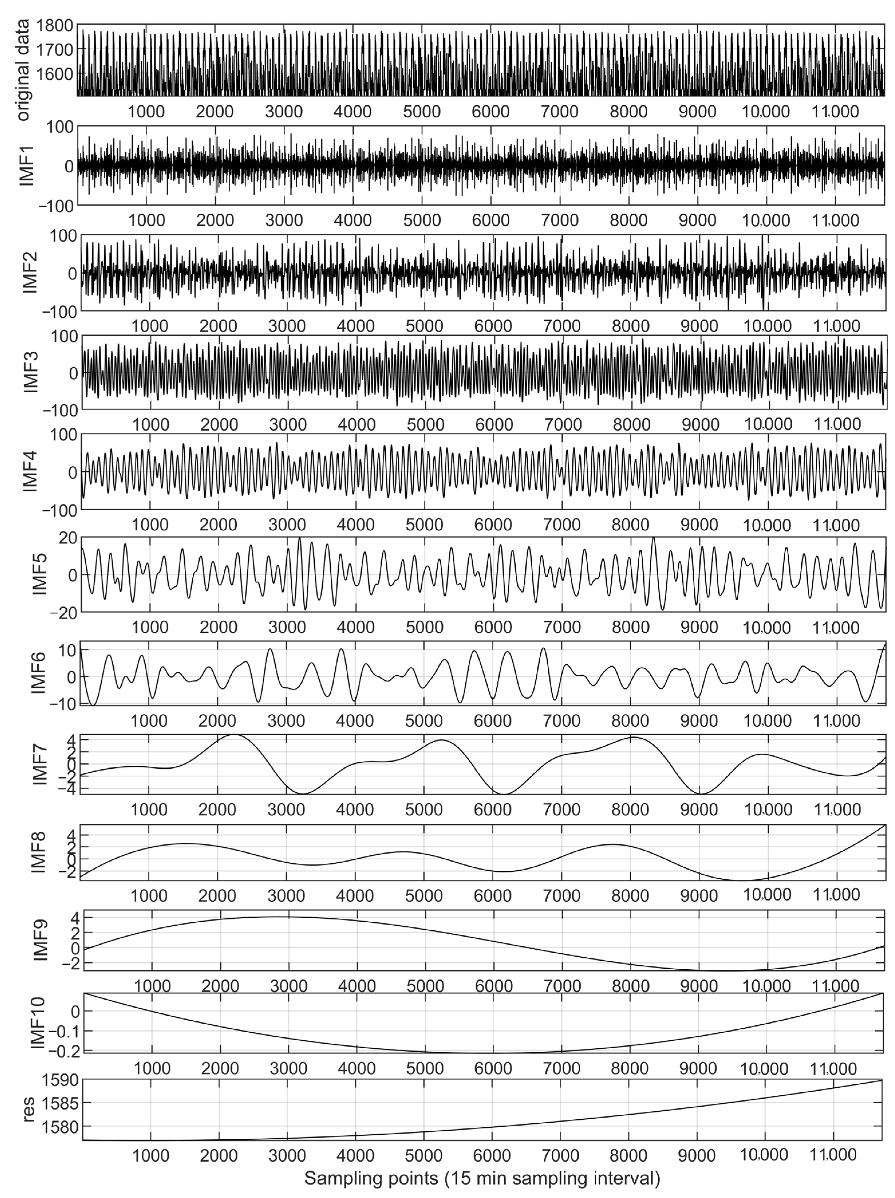
In this paper, the original power load data are denoised and then decomposed according to the CEEMD process to obtain the intrinsic modal components IMF1~IMF7 with different fluctuation scale information of the original residual series. Figure 9 shows each modal component after the CEEMD model is decomposed.
In general, the reconstruction of IMF components is based on subjective experience to determine the reconstruction method. However, this method is not suitable for power load decomposition and reconstruction. Therefore, this paper retains all component signals and establishes MNet-Atten time series prediction models for different IMF components for prediction.

5.3. Comparative Study and Analysis of Different Load Decomposition Methods

In order to verify the advantages of the composite decomposition method proposed in this paper, the decomposition without decomposition, EMD decomposition [34], EEMD decomposition [35], CEEMD decomposition [36], and the decomposition proposed in this paper are used as the comparison load decomposition methods. The comparison of the prediction results of different modal decomposition methods with the proposed model is shown in Table 3.
Decomposition using the EMD method will lead to overlapping between different modes, and the extraction effect of load change features is limited. Decomposition using the EEMD method has the problem of large reconstruction error, which affects the accuracy of prediction. As can be seen from Table 3, the evaluation indexes of the EMD method in load forecasting are all worse than those without load decomposition and using the EEMD method. Based on the EMD method, combining the EEMD method with the EEMD method, the problems of modal aliasing in the EMD method and large reconstruction error in the EEMD method are avoided by introducing adaptive noise control and multiple iterations. In addition, compared with the EEMD decomposition method, the CEEMD method corresponds to better prediction performance.
The combination of CEEMD and SVD improves the model performance, which indicates that the SVD method promotes the extraction of signal features and reduces data volatility. Taking the evaluation indexes MAPE and RMSE as an example, compared with no modal decomposition, EMD decomposition, EEMD decomposition, and CEEMD decomposition, the MAPE of this paper’s method is reduced by 1.2049, 0.8632, 0.6791, and 0.5360, and the RMSE is reduced by 4.5952, 3.3381, 2.3830, and 21.62%, respectively. The results show that the proposed prediction model based on the composite decomposition algorithm of CEEMD + SVD performs optimally, which verifies the effectiveness of the proposed load decomposition method.

5.4. Analysis of Simulation Results

In order to verify the performance advantages of the prediction model proposed in this paper, the prediction model proposed in this paper is compared with other prediction models. The employed prediction models include SVM [37], XGBoost [38], BPNN [39], TCN [40], CNN [41], and GRU [42]. Each comparison model uses the same training set, validation set, and test set as inputs to the proposed model. Additionally, the same preprocessing and feature screening methods are applied to the input data to ensure consistency and comparability among the models. A comparison of the prediction results of the single model and the model in this paper is shown in Table 4. From Table 4, it can be seen that the proposed model has the best performance among all the prediction models and is more accurate than the SVM, XGBoost, BPNN, TCN, CNN, and GRU models, i.e., the prediction results of this method are closer to the actual values.
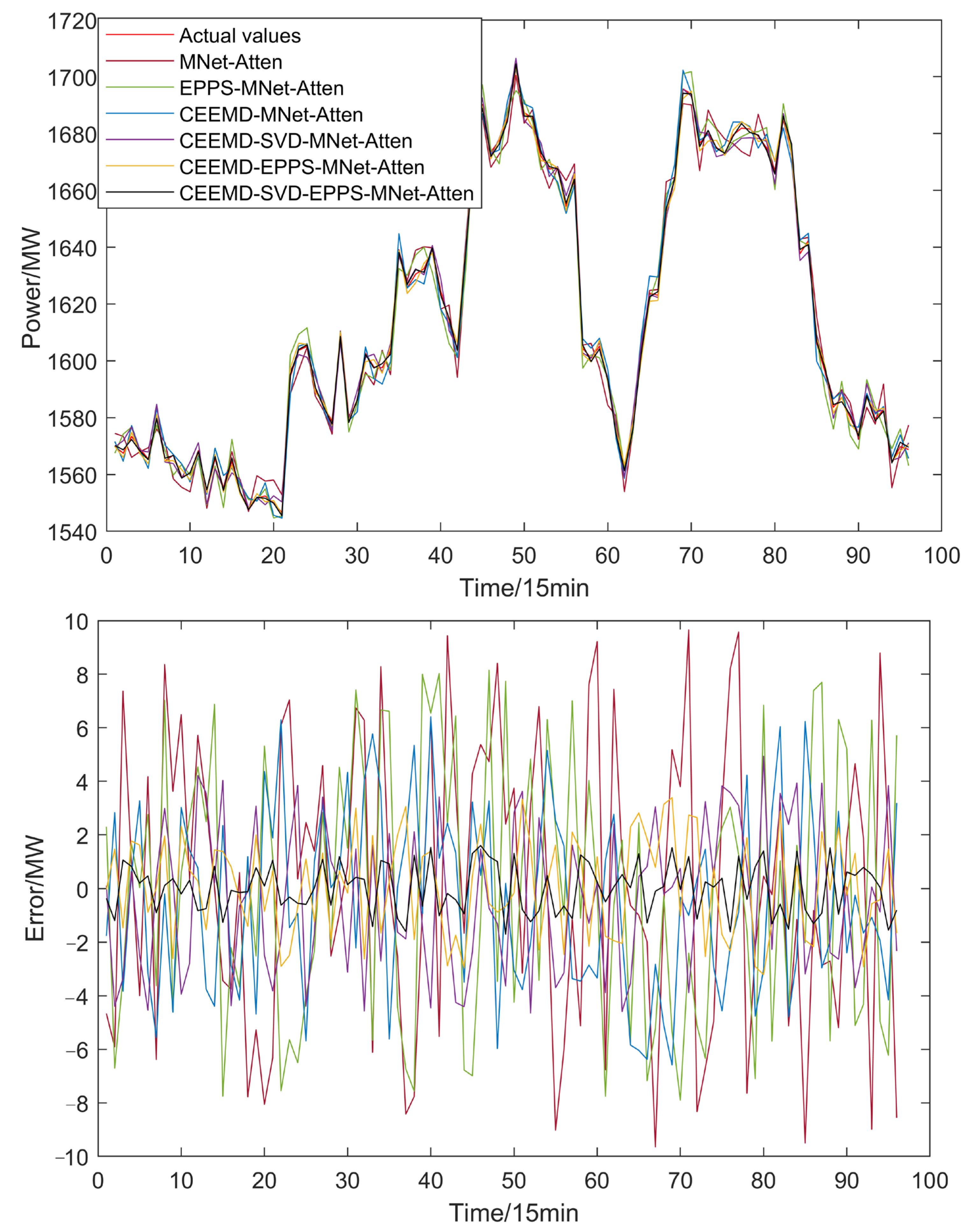
In addition, two groups of model combinations are used to verify the validity of the model CEEMD-SVD-EPPS-MNet-Atten constructed in this paper. The first group is based on a horizontal comparison of the model combinations presented in this paper. Six model combinations, CEEMD-SVD-EPPS-MNet-Atten, CEEMD-EPPS-MNet-Atten, CEEMD-SVD-MNet-Atten, CEEMD-MNet-Atten, EPPS-MNet-Atten, and MNet-Atten, are developed in this paper. The models are also evaluated using evaluation metrics, i.e., Equations (30)–(32). Figure 10 shows a comparative presentation of predicted data and actual values for the six model combinations, and Table 5 shows the evaluation results of the six model combinations.
The comparison shows that the single model MNet-Atten has the worst prediction results, while the accuracy of the prediction results is significantly improved after the sequence decomposition by CEEMD or after the parameters are optimized by the EPPS algorithm. Nevertheless, both the CEEMD-MNet-Atten model without EPPS optimization and the EPPS-MNet-Atten model without CEEMD treatment are inferior to the CEEMD-EPPS-MNet-Atten model in prediction accuracy. To further improve the load forecasting accuracy, the SVD algorithm is introduced in this paper for noise reduction of the data. The comparison of the CEEMD-MNet-Atten model with the CEEMD-SVD-MNet-Atten model or the CEEMD-EPPS-MNet-Atten model with the CEEMD-SVD-EPPS-MNet-Atten model confirms that the prediction error becomes smaller after the introduction of SVD. In addition, the average value of 30 running times of the combined model proposed in this paper is 117.3231 s, which is much smaller than the 149.7716 s running time of the combined CEEMD-EPPS-MNet-Atten model, which dramatically saves the computation time. Moreover, the correlation coefficient PCC of the CEEMD-SVD-EPPS-MNet-Atten model is closer to 1. The above analysis proves that the CEEMD-SVD-EPPS-MNet-Atten model constructed in this paper has a better prediction performance.
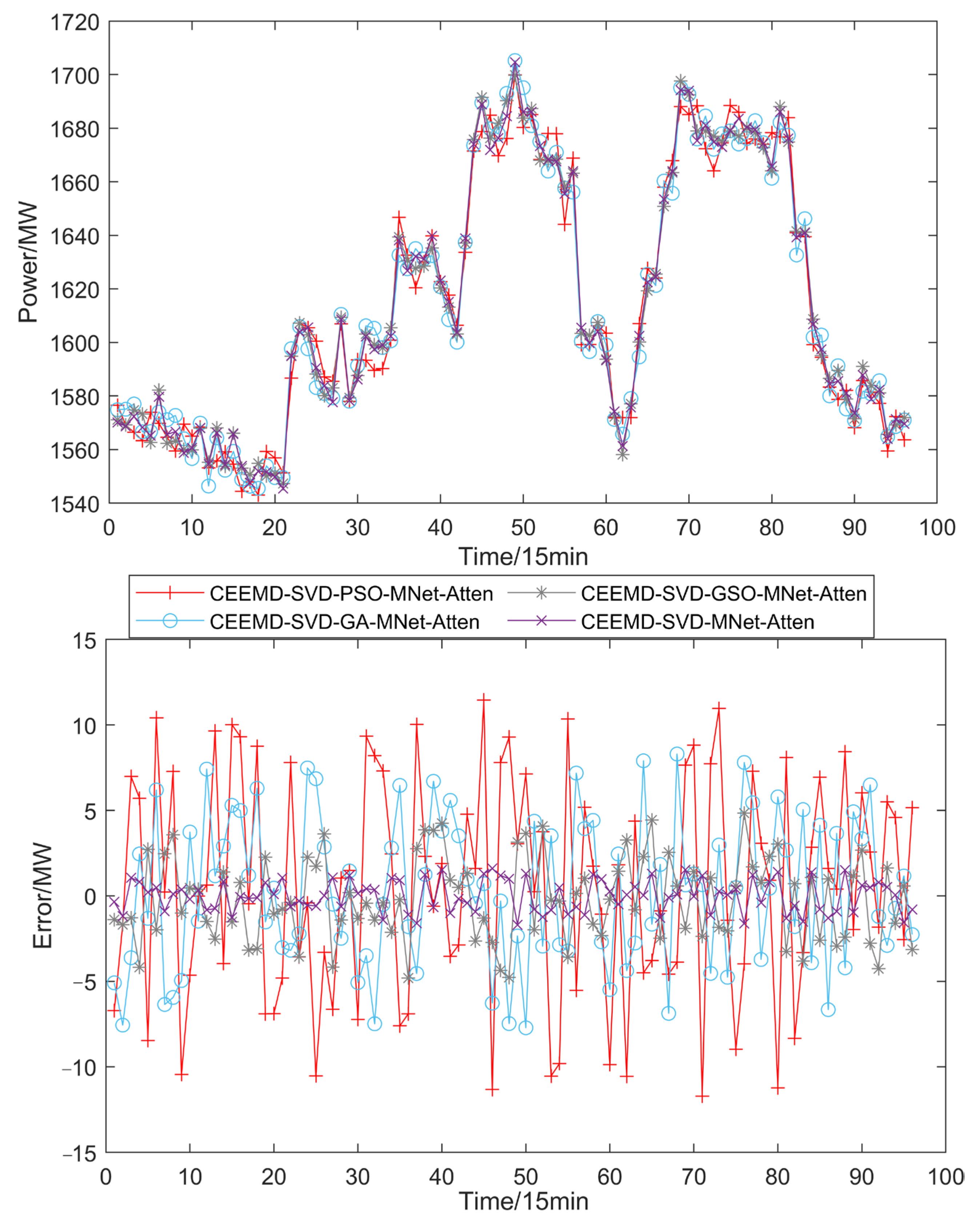
The second group is based on a longitudinal comparison of the model combinations presented in this paper. A comparison of the three models CEEMD-SVD-PSO-MNet-Atten, CEEMD-SVD-GA-MNet-Atten, and CEEMD-SVD-GSO-MNet-Atten with the proposed model CEEMD-SVD-EPPS-MNet-Atten is performed. Table 6 displays the evaluation results of the four models, and Figure 11 exhibits the prediction curves for the four models. The comparison shows that the CEEMD-SVD-EPPS-MNet-Atten model has the lowest MAPE, RMSE, and PCC. The MAPE is 2.1372% lower than that of CEEMD-SVD-PSO-MNet-Atten, 0.8959% lower than that of CEEMD-SVD-GA-MNet-Atten, and 0.4071% lower than that of CEEMD-SVD-GSO-MNet-Atten.
Figure 12 displays the heat map to present the comparison results of the CEEMD-SVD-PSO-MNet-Atten, CEEMD-SVD-GA-MNet-Atten, CEEMD-SVD-GSO-MNet-Atten, and CEEMD-SVD-EPPS-MNet-Atten. As can be seen from Figure 11, the color of the error obtained from the CEEMD-SVD-PSO-MNet-Atten model is relatively rich, with a comparatively large error value. The color of the error obtained from the CEEMD-SVD-EPPS-MNet-Atten model is relatively uniform, closer to zero, indicating a smaller error value and a lower average. In summary, the model optimized by EPPS has the best prediction effect compared with the currently used evolutionary algorithms.

6. Conclusions

In this paper, based on the periodicity and volatility of power load changes, the optimized EPPS-MNet-Atten for short-term power load forecasting is constructed based on the CEEMD and MNet-Atten algorithms combined with the SVD and EPPS algorithms for power load forecasting. Based on the advantages of CEEMD, SVD is used for decomposition and reconstruction to preserve the features of the original data and achieve the main component extraction. Taking the evaluation metrics MAPE and RMSE as examples, compared to performing no modal decomposition, as well as to EMD, EEMD, and CEEMD decomposition methods, the proposed approach reduces MAPE by 1.2049, 0.8632, 0.6791, and 0.5360, and lowers RMSE by 4.5952, 3.3381, 2.3830, and 21.62%, respectively. This process completes the data noise reduction processing, ensuring prediction accuracy and accommodating the prediction rate. The proposed model outperforms all other comparative models, namely SVM, XGBoost, BPNN, TCN, CNN, and GRU, in terms of prediction accuracy. Furthermore, the learning rate of the MNet-Atten model is optimized using the EPPS algorithm, which has a strong optimization capability and fast convergence speed, resulting in a better optimization performance than previous optimization algorithms and improving the prediction accuracy. The comparison shows that the CEEMD-SVD-EPPS-MNet-Atten model has the lowest MAPE, RMSE, and PCC. The MAPE is 2.1372% lower than that of CEEMD-SVD-PSO-MNet-Atten, 0.8959% lower than that of CEEMD-SVD-GA-MNet-Atten, and 0.4071% lower than that of CEEMD-SVD-GSO-MNet-Atten. To sum up, the model proposed in this paper has a higher prediction accuracy than a general single model or a combined model without in-depth processing. In the future, the possible influencing factors for the load data will be further studied and substituted into the prediction model to optimize the model and reduce the prediction error. Furthermore, the current choice of the summation ratio of the nonlinear layers is based on a priori assumptions; its experimental derivation for optimal values and correlation with data characteristics represent a valuable future research direction.

Author Contributions

Conceptualization, X.W. and Q.J.; methodology, Q.J.; validation, H.X. and X.K.; formal analysis, X.W.; investigation, Q.J.; data curation, H.X. and X.K.; writing—original draft preparation, X.W.; writing—review and editing, Q.J.; visualization, X.K.; supervision, X.W.; project administration, X.W. All authors have read and agreed to the published version of the manuscript.

Funding

This research was funded by the Shandong Provincial Key R&D Program (grant number 2019JZZY020804) and the Shandong Provincial Innovation Capacity Enhancement Programme for Science and Technology-Based Small and Medium-sized Enterprises (grant number 2023TSGC1014).

Data Availability Statement

The original contributions presented in this study are included in the article. Further inquiries can be directed to the corresponding author.

Conflicts of Interest

Qi Jiang was employed by the Shandong Deyou Electric Co., Ltd. Huaitang Xia and Xianbo Kong were employed by the Shandong Chenxiang Electric Equipment Co., Ltd. Xiaobin Wei declares that the research was conducted in the absence of any commercial or financial relationships that could be construed as a potential conflict of interest.

References

  1. Wang, C.; Wang, Y.; Song, F. Research on Electric Vehicle Charging Load Forecasting Method Based on Improved LSTM Neural Network. World Electr. Veh. J. 2025, 16, 265. [Google Scholar] [CrossRef]
  2. Ma, P.; Cui, S.; Chen, M.; Zhou, S.; Wang, K. Review of family-level short-term load forecasting and its application in household energy management system. Energies 2023, 16, 5809. [Google Scholar] [CrossRef]
  3. Habbak, H.; Mahmoud, M.; Metwally, K.; Fouda, M.; Ibrahem, M. Load forecasting techniques and their applications in smart grids. Energies 2023, 16, 1480. [Google Scholar] [CrossRef]
  4. Dewangan, F.; Abdelaziz, A.Y.; Biswal, M. Load forecasting models in smart grid using smart meter information: A review. Energies 2023, 16, 1404. [Google Scholar] [CrossRef]
  5. Tarmanini, C.; Sarma, N.; Gezegin, C.; Ozgonenel, O. Short term load forecasting based on ARIMA and ANN approaches. Energy Rep. 2023, 9, 550–557. [Google Scholar] [CrossRef]
  6. Wan, A.; Chang, Q.; Khalil, A.; He, J. Short-term power load forecasting for combined heat and power using CNN-LSTM enhanced by attention mechanism. Energy 2023, 282, 128274. [Google Scholar] [CrossRef]
  7. Wei, N.; Yin, C.; Yin, L.; Tan, J.; Liu, J.; Wang, S.; Qiao, W.; Zeng, F. Short-term load forecasting based on WM algorithm and transfer learning model. Appl. Energy 2024, 353, 122087. [Google Scholar] [CrossRef]
  8. Sun, Y.; Tian, X.; Bao, W.; Qu, S.; Li, Q.; Chen, Y.; Shi, P. Improving the forecast performance of hydrological models using the cubature Kalman filter and unscented Kalman filter. Water Res. Res. 2023, 59, e2022WR033580. [Google Scholar] [CrossRef]
  9. Junior, M.; Freire, R.; Seman, L.; Stefenon, S.; Mariani, V.; Coelho, L. Optimized hybrid ensemble learning approaches applied to very short-term load forecasting. Int. J. Electr. Power Energy Syst. 2024, 155, 109579. [Google Scholar] [CrossRef]
  10. Bartwal, D.; Sindhwani, R.; Vaidya, O. Improving forecast accuracy for seasonal products in FMCG industry: Integration of SARIMA and regression model. Int. J. Ind. Sys. Eng. 2024, 46, 259–279. [Google Scholar] [CrossRef]
  11. Zhang, J. Utilizing gaussian process regression model enhanced by metaheuristic algorithms to forecast undrained shear strength. J. Appl. Sci. Eng. 2025, 28, 741–752. [Google Scholar] [CrossRef]
  12. Bacanin, N.; Stoean, C.; Zivkovic, M. On the benefits of using metaheuristics in the hyperparameter tuning of deep learning models for energy load forecasting. Energies 2023, 16, 1434. [Google Scholar] [CrossRef]
  13. Abedinia, O.; Amjady, N.; Shafie-Khah, M. Electricity price forecast using combinatorial neural network trained by a new stochastic search method. Energy Convers. Manag. 2015, 105, 642–654. [Google Scholar] [CrossRef]
  14. Huang, N.; Wang, S.; Wang, R.; Cai, G.; Liu, Y.; Dai, Q. Gated spatial-temporal graph neural network based short-term load forecasting for wide-area multiple buses. Int. J. Electr. Power Energy Syst. 2023, 145, 108651. [Google Scholar] [CrossRef]
  15. Ullah, K.; Ahsan, M.; Hasanat, S.; Haris, M.; Yousaf, H.; Raza, S. Short-term load forecasting: A comprehensive review and simulation study with CNN-LSTM hybrids approach. IEEE Access 2024, 12, 111858–111881. [Google Scholar] [CrossRef]
  16. Wazirali, R.; Yaghoubi, E.; Abujazar, M.; Rami, A.; Vakili, A. State-of-the-art review on energy and load forecasting in microgrids using artificial neural networks, machine learning, and deep learning techniques. Electr. Power Syst. Res. 2023, 225, 109792. [Google Scholar] [CrossRef]
  17. Lotfipoor, A.; Patidar, S.; Jenkins, D. Deep neural network with empirical mode decomposition and Bayesian optimisation for residential load forecasting. Expert Syst. Appl. 2024, 237, 121355. [Google Scholar] [CrossRef]
  18. Zhang, Q.; Wu, J.; Ma, Y.; Li, G.; Ma, J.; Wang, C. Short-term load forecasting method with variational mode decomposition and stacking model fusion. Sus. Energy Grids Netw. 2022, 30, 100622. [Google Scholar] [CrossRef]
  19. Liu, Q.; Cao, J.; Zhang, J.; Zhong, Y.; Ba, T.; Zhang, Y. Short-term power load forecasting in FGSM-Bi-LSTM networks based on empirical wavelet transform. IEEE Access 2023, 11, 105057–105068. [Google Scholar] [CrossRef]
  20. Shi, J.; Teh, J. Load forecasting for regional integrated energy system based on complementary ensemble empirical mode decomposition and multi-model fusion. Appl. Energy 2024, 353, 122146. [Google Scholar] [CrossRef]
  21. Li, K.; Duan, P.; Cao, X.; Cheng, Y.; Zhao, B.; Xue, Q.; Feng, M. A multi-energy load forecasting method based on complementary ensemble empirical model decomposition and composite evaluation factor reconstruction. Appl. Energy 2024, 365, 123283. [Google Scholar] [CrossRef]
  22. Xiang, Y.; Zhuang, X.H. Application of ARIMA model in short-term prediction of international crude oil price. Adv. Mater. Res. 2013, 798, 979–982. [Google Scholar] [CrossRef]
  23. Murat, A.; Tokat, E. Forecasting oil price movements with crack spread futures. Energy Econ. 2009, 31, 85–90. [Google Scholar] [CrossRef]
  24. Nugroho, D.B.; Setiawan, A.; Morimoto, T. Modelling and Forecasting Financial Volatility with Realized GARCH Model: A Comparative Study of Skew-t Distributions Using GRG and MCMC Methods. Econometrics 2025, 13, 33. [Google Scholar] [CrossRef]
  25. Cavicchioli, M. Forecasting Markov switching vector autoregressions: Evidence from simulation and application. J. Forecast. 2025, 44, 136–152. [Google Scholar] [CrossRef]
  26. Pukach, A.; Teslyuk, V.; Lysa, N.; Sikora, L.; Fedyna, B. Information-Cognitive Concept of Predicting Method for HCI Objects’ Perception Subjectivization Results Based on Impact Factors Analysis with Usage of Multilayer Perceptron ANN. Appl. Sci. 2025, 15, 9763. [Google Scholar] [CrossRef]
  27. Jedrzejczyk, A.; Firek, K.; Rusek, J. Prediction of damage intensity to masonry residential buildings with convolutional neural network and support vector machine. Sci. Rep. 2024, 14, 16256. [Google Scholar] [CrossRef]
  28. Li, X.; Wang, J. Predicting Constitutive Behaviour of Idealized Granular Soils Using Recurrent Neural Networks. Appl. Sci. 2025, 15, 9495. [Google Scholar] [CrossRef]
  29. Jang, M.; Joo, S.-K. Pattern-Aware BiLSTM Framework for Imputation of Missing Data in Solar Photovoltaic Generation. Energies 2025, 18, 4734. [Google Scholar] [CrossRef]
  30. Jha, A.; Ray, D.; Sarkar, D.; Prakash, T.; Dewangan, N. Bidirectional long-short-term memory-based fractional power system stabilizer: Design, simulation, and real-time validation. Int. J. Numer. Model. Electron. Netw. Devices Fields 2024, 37, 3300. [Google Scholar] [CrossRef]
  31. Chen, J.; Wu, Q.; Ji, T.; Wu, P.; Li, M. Evolutionary predator and prey strategy for global optimization. Inf. Sci. 2016, 327, 217–232. [Google Scholar] [CrossRef]
  32. Wang, L.; Xie, M.; Pan, M.; He, F.; Yang, B.; Gong, Z.; Wu, X.; Shang, M.; Shan, K. Improved Deep Learning Predictions for Chlorophyll Fluorescence Based on Decomposition Algorithms: The Importance of Data Preprocessing. Water 2023, 15, 4104. [Google Scholar] [CrossRef]
  33. Chen, L.Y.; Wang, C.; Xiao, X.Y.; Ren, C.; Zhang, D.J. Denoising in SVD-based ghost imaging. Opt. Express 2022, 30, 6248–6257. [Google Scholar] [CrossRef]
  34. Zeng, S.; Cui, J.; Luo, D.; Lu, N. Bridge Damage Identification Using Time-Varying Filtering-Based Empirical Mode Decomposition and Pre-Trained Convolutional Neural Networks. Sensors 2025, 25, 4869. [Google Scholar] [CrossRef]
  35. Guo, Y.; Si, J.; Wang, Y. Ensemble-Empirical-Mode-Decomposition (EEMD) on SWH prediction: The effect of decomposed IMFs, continuous prediction duration, and data-driven models. Ocean Eng. 2025, 324, 120755. [Google Scholar] [CrossRef]
  36. Xu, Y.; Li, H.; Meng, X.; Chen, J.; Zhang, X.; Peng, T. An Energy System Modeling Approach for Power Transformer Oil Temperature Prediction Based on CEEMD and Robust Deep Ensemble RVFL. Processes 2025, 13, 2487. [Google Scholar] [CrossRef]
  37. Yang, X.; Meng, P.; Jiang, Z.; Zhou, L. Deep siamese residual support vector machine with applications to disease prediction. Comput. Biol. Med. 2025, 196, 110693. [Google Scholar] [CrossRef] [PubMed]
  38. Peng, Y.; Kai, J.; Yu, X.; Zhang, Z.; Li, Q.J.; Yang, G.; Kong, L. Pavement Friction Prediction Based Upon Multi-View Fractal and the XGBoost Framework. Lubricants 2025, 13, 391. [Google Scholar] [CrossRef]
  39. Fauzan, A.N.; Assahari, M.S.; Jainun, A.R.; Somantri. Backpropagation Neural Network Algorithm for Optimizing Network Bandwidth Allocation Based on User Access Patterns. Eng. Proc. 2025, 107, 56. [Google Scholar] [CrossRef]
  40. Han, H.; Peng, J.; Ma, J.; Liu, H.; Liu, S. Research on Load Forecasting Prediction Model Based on Modified Sand Cat Swarm Optimization and SelfAttention TCN. Symmetry 2025, 17, 1270. [Google Scholar] [CrossRef]
  41. Li, H.; Li, S.; Li, H.; Bai, L. Ultra-Short-Term Wind Power Prediction Based on Fused Features and an Improved CNN. Processes 2025, 13, 2236. [Google Scholar] [CrossRef]
  42. Sun, R.; Huang, Z.; Liang, X.; Zhu, S.; Li, H. A GRU-Enhanced Kolmogorov–Arnold Network Model for Sea Surface Temperature Prediction Derived from Satellite Altimetry Product in South China Sea. Remote Sens. 2025, 17, 2916. [Google Scholar] [CrossRef]
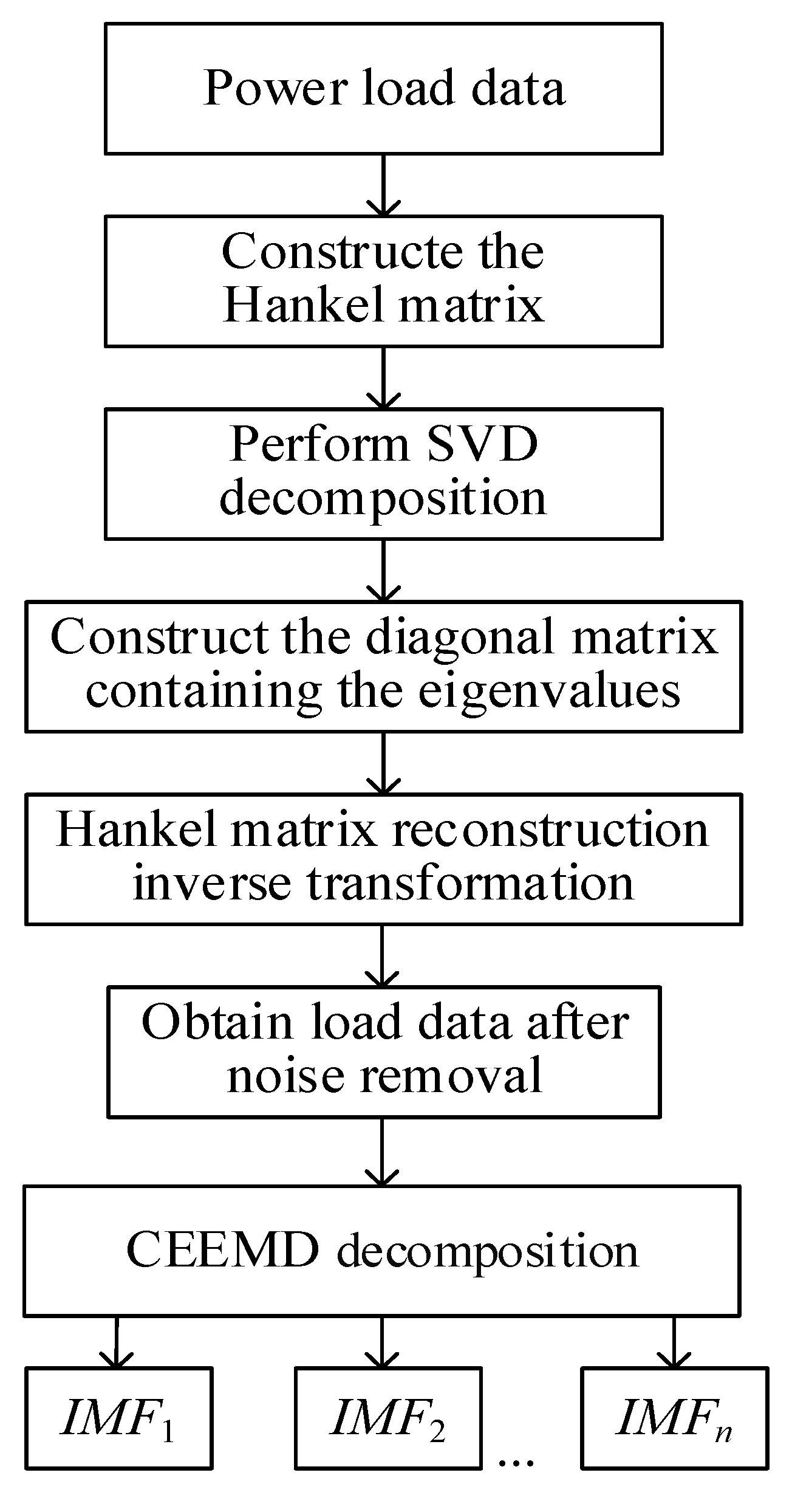
Figure 1. Composite decomposition model based on SVD-CEEMD.
Wevj 16 00564 g001
Figure 2. Structure of long term and short-term temporal networks with attention.
Wevj 16 00564 g002
Figure 3. Schematic diagram of BiGRU structure.
Wevj 16 00564 g003
Figure 4. Structure of temporal pattern attention mechanism.
Wevj 16 00564 g004
Figure 5. The flowchart of MNet-Atten based on optimization of the evolutionary predator and prey strategy.
Wevj 16 00564 g005
Figure 6. The short-term electric vehicle charging load forecasting flowchart.
Wevj 16 00564 g006
Figure 7. Presentation of a sample of data sets.
Wevj 16 00564 g007
Figure 8. Contrast of de-noised and historical data.
Wevj 16 00564 g008
Figure 9. CEEMD decomposition results of power load.
Wevj 16 00564 g009
Figure 10. Comparison of prediction results of six models.
Wevj 16 00564 g010
Figure 11. Comparison of prediction results of four models.
Wevj 16 00564 g011
Figure 12. Heat map of prediction results for four models.
Wevj 16 00564 g012
Table 1. Survey of previous studies.
ModelReferenceCategoryAdvantagesDisadvantages
AutoRegressive Integrated Moving Average Model (ARIMA)[22]Traditional Statistical Model1. Solid theoretical foundation, clear statistical properties, and strong interpretability.
2. Excellent ability to capture linear relationships, especially suitable for stationary time series with obvious trends and seasonality.
3. Model parameters have clear statistical meanings.
4. Serves as a benchmark model for handling univariate time series.
1. Only applicable to univariate time series and cannot directly utilize multivariate information.
2. Requires the series to be stationary or stationary after differencing, demanding high-quality data preprocessing.
3. Assumes a linear relationship between series, making it ineffective in capturing complex nonlinear patterns.
4. The process of model identification and order determination requires certain experience and statistical knowledge.
Random Walk (RW)[23]Traditional Statistical Model1. Extremely simple model with no need for parameter estimation.
2. Acts as an effective benchmark model for many financial time series and is often difficult to outperform.
3. Embodies the philosophical idea that “the future is unpredictable” and serves as a crucial tool for testing the effectiveness of forecasting models.
1. Extremely low practicality except when used as a benchmark. It simply uses the current value as the best prediction for the next moment.
2. Predictions form a horizontal line, making it unable to forecast trends and fluctuations.
3. The variance of prediction errors increases infinitely over time.
Generalized Autoregressive Conditional Heteroskedasticity Model (GARCH)[24]Traditional Statistical Model1. Specifically designed to characterize and forecast volatility (variance), rather than the series values themselves.
2. Can accurately capture volatility clustering (large fluctuations followed by large fluctuations, small fluctuations followed by small fluctuations) in financial time series.
3. Provides a key tool for fields such as risk management and option pricing.
1. Mainly used for volatility modeling and usually needs to be combined with models such as ARIMA (ARIMA-GARCH) to simultaneously forecast mean and variance.
2. Sensitive to model parameters and has a relatively complex setup.
3. Also based on the linear assumption, which may lead to insufficient forecasting of extreme events.
Vector Autoregression Model (VAR)[25]Traditional Statistical Model1. Naturally handles multivariate time series and can capture bidirectional dynamic relationships between variables.
2. Concise model form, where all variables are treated equally, facilitating estimation and understanding.
3. Can be used to analyze Granger causality and impulse response between variables.
1. A large number of parameters. When the number of variables is K and the lag order is p, the number of parameters is K2p, which easily leads to overfitting (the “curse of dimensionality”).
2. Also requires the system to be stationary and relies heavily on the linear relationship assumption.
3. Highly sensitive to the selection of predictive variables.
Artificial Neural Network (ANN)[26]Machine Learning Model1. Follows the universal approximation theorem, enabling it to approximate any complex nonlinear mapping relationship with arbitrary precision.
2. Has loose requirements on data distribution assumptions, without the need for strict conditions such as stationarity required by traditional models.
3. Strong robustness to noisy data.
1. A “black-box” model with extremely poor interpretability, making it difficult to understand its internal decision-making logic.
2. Requires a large amount of data for training and is prone to overfitting when the data volume is small.
3. The training process involves large computational costs, and parameter tuning (network structure, learning rate, etc.) is complex, requiring numerous experiments.
Support Vector Machine (SVM)[27]Machine Learning Model1. Based on the principle of structural risk minimization, it has strong generalization ability, performs well on small-sample datasets, and is not prone to overfitting.
2. Can efficiently handle nonlinear problems through kernel tricks.
3. Capable of finding global optimal solutions rather than local optimal ones.
1. Training speed decreases sharply with the increase in data volume, and it consumes a great deal of memory, making it unsuitable for ultra-large-scale datasets.
2. Sensitive to the selection of parameters, so parameter tuning is crucial.
3. Essentially a binary classification model; its performance and efficiency decline when used for regression (SVR) and multi-class classification tasks.
4. The interpretability of results remains relatively poor.
Recurrent Neural Network (RNN)[28]Deep Learning Model1. Specifically designed for sequence data, with memory functionality, enabling it to make predictions using information from all historical time steps.
2. Parameter sharing mechanism significantly reduces the number of model parameters.
3. Theoretically capable of capturing temporal dependencies of any length.
1. Suffers from the problem of gradient vanishing/explosion, making it difficult to effectively learn long term dependencies (e.g., when information from a long time ago has a significant impact on current predictions, it cannot capture this effectively).
2. The training and computation process is sequential, making parallelization difficult and resulting in slow training speed.
LSTM (Long Short-Term Memory Network)[29]Deep Learning Model1. Perfectly solves the gradient vanishing problem of RNN, enabling effective learning of long term dependencies and serving as a milestone model in time series forecasting.
2. Precisely controls the flow and memory of information through the “gating” mechanism (input gate, forget gate, output gate).
1. The model is highly complex with a large number of parameters, leading to high training costs (in terms of time and computing resources).
2. Requires an extremely large amount of data to train an effective model; otherwise, severe overfitting will occur.
BiLSTM (Bidirectional LSTM)[30]Deep Learning ModelBiLSTM can simultaneously utilize contextual information from the past and future, resulting in stronger feature extraction capabilities and often higher accuracy.1. The model is highly complex with a large number of parameters, leading to high training costs (in terms of time and computing resources).
2. Requires an extremely large amount of data to train an effective model; otherwise, severe overfitting will occur.
Table 2. The pseudocode of MNet-Atten based on optimization of evolutionary predator and prey strategy.
1: Initialize model parameters; set the initialization parameters for the EPPS algorithm.
2: Train the MNet-Atten network.
3: Return fitness values to EPPS.
4: Utilize the search mechanism to update population individuals.
5: Reach the maximum number of iterations or the fitness function.
6: Enter the optimal learning rate.
7: Extracts both short- and long term dependencies within the data.
8: Employ a temporal attention mechanism to focus on key sequences while filtering out distracting elements.
9: Extract the linear features of the sequence from the autoregressive model.
10: Combine the results of the nonlinear and linear components to obtain the forecast outcome.
11: Calculate the error between the output value and the target value.
12: Meet the requirements of the error and obtain the forecast results.
Table 3. Comparison of prediction results of the proposed model and other decomposition methods.
MethodMAPERMSEPCC
Without the decomposition method2.13446.753895.3642
EMD decomposition method1.79275.496796.3758
EEMD decomposition method1.60864.541697.6602
CEEMD decomposition method1.46553.980598.5126
The proposed decomposition method0.92951.821999.2387
Table 4. Comparison of the prediction results of the proposed model and other models.
MethodMAPERMSEPCC
SVM3.46816.530496.5514
XGBoost2.72365.692797.0046
BPNN2.40154.365197.2893
TCN1.91223.279898.0904
CNN2.24675.328697.5033
GRU1.68392.880398.2237
The proposed method0.92951.821999.2387
Table 5. The evaluation results of the six model combinations.
ModelMAPERMSEPCC
MNet-Atten1.80125.125898.2326
EPPS-MNet-Atten1.43264.986498.4579
CEEMD-MNet-Atten1.24353.861598.5744
CEEMD-SVD-MNet-Atten1.06113.412798.7803
CEEMD-EPPS-MNet-Atten0.98092.459199.0897
CEEMD-SVD-EPPS-MNet-Atten0.92952.158699.2387
Table 6. The evaluation results of the four models.
ModelMAPERMSEPCC
CEEMD-SVD-PSO-MNet-Atten0.94982.197998.8721
CEEMD-SVD-GA-MNet-Atten0.93762.178199.1417
CEEMD-SVD-GSO-MNet-Atten0.93332.178499.2109
CEEMD-SVD-EPPS-MNet-Atten0.92952.158699.2387
Disclaimer/Publisher’s Note: The statements, opinions and data contained in all publications are solely those of the individual author(s) and contributor(s) and not of MDPI and/or the editor(s). MDPI and/or the editor(s) disclaim responsibility for any injury to people or property resulting from any ideas, methods, instructions or products referred to in the content.