Stability Study of Distributed Drive Vehicles Based on Estimation of Road Adhesion Coefficient and Multi-Parameter Control

Abstract

In order to improve the driving stability of distributed-drive intelligent electric vehicles under different roadway attachment conditions, this paper proposes a multi-parameter control algorithm based on the estimation of road adhesion coefficients. First, a seven-degree-of-freedom (7-DOF) vehicle dynamics model is established and optimized with a layered control strategy. The upper-level control module calculates the desired yaw rate and sideslip angle using the two-degree-of-freedom (2-DOF) vehicle model and estimates the road adhesion coefficient by using the singular-value optimized cubature Kalman filtering (CKF) algorithm; the middle-level utilizes the second-order sliding mode controller (SOSMC) as a direct yaw moment controller in order to track the desired yaw rate and sideslip angle while also employing a joint distribution algorithm to control the torque distribution based on vehicle stability parameters, thereby enhancing system robustness; and the lower-level controller performs optimal torque allocation based on the optimal tire loading rate as the objective. A Speedgoat-CarSim hardware-in-the-loop simulation platform was established, and typical driving scenarios were simulated to assess the stability and accuracy of the proposed control algorithm. The results demonstrate that the proposed algorithm significantly enhances vehicle-handling stability across both high- and low-adhesion road conditions.

1. Introduction

Distributed-drive intelligent electric vehicles, which utilize hub motors and wheel-side motors as their primary drive units, offer notable advantages in terms of chassis design and integrated control. However, the uncertainties in road adhesion coefficients and the nonlinear coupling behaviors of tires present significant challenges in controller design [1,2]. In response to the increasing demand for active safety control in modern vehicles, driving state estimation using low-cost sensors has emerged as a critical foundation for enabling efficient safety management [3]. Distributed-drive electric vehicles, with their enhanced control flexibility, compactness, and high transmission efficiency, provide robust hardware support for improving handling stability through techniques such as direct yaw moment control (DYC) and traction control systems (TCSs). Recent advancements in active chassis control systems have led to substantial improvements in vehicle stability and safety, particularly under complex driving conditions [4,5,6].

The road adhesion coefficient is a critical parameter in vehicle dynamic control systems, as its accurate estimation is essential for improving vehicle stability, maneuverability, and safety. Existing approaches for estimating this coefficient can be broadly categorized into two groups: experiment-based methods and model-based methods [7]. Experiment-based methods tend to provide more accurate estimates under conditions of small excitation signals and can even predict the adhesion coefficient before the wheels make contact with the road. However, in real-world applications, the vehicle environment is highly complex, and many high-precision sensors are susceptible to noise and other disturbances. Methods that use image processing or noise analysis to identify the road adhesion coefficient typically require large datasets, resulting in high engineering costs and limiting their practical applicability. Consequently, model-based estimation methods have become the focus of a lot of recent research. These methods use common onboard sensors (e.g., wheel speed sensors, accelerometers) to monitor the vehicle’s motion state and then indirectly estimate the adhesion coefficient by establishing a relationship between the vehicle’s dynamic model and the road adhesion coefficient [8]. Among these methods, the Kalman filter (KF) and its variants have been widely applied for this purpose [9]. For example, Wu [10] of Jilin University proposed an estimation algorithm based on the extended Kalman filter (EKF), which first estimates the vehicle’s driving state parameters and then derives the road adhesion coefficient using the relationship between the vehicle state and road conditions. The EKF is an extension of the KF that is designed for nonlinear systems. It approximates the system’s state transition and observation models by performing a first-order Taylor expansion of the nonlinear functions. While it provides good estimates, its reliance on local linearization of nonlinear systems can lead to a decrease in estimation accuracy in the presence of strong nonlinearities [11]. To overcome this limitation, Wang et al. [12] introduced the unscented Kalman filter (UKF), which performs an unbiased transformation using a set of sigma points, avoiding errors from linearization and maintaining high accuracy in complex, nonlinear systems. However, UKF may suffer from loss of statistical properties of the posterior distribution in high-dimensional systems and is prone to issues such as non-positive definiteness, which can cause estimation instability [13]. To address these challenges, Zhang et al. [14] proposed a new tire model and improved the accuracy of the adhesion coefficient estimate using an enhanced cubature Kalman filter (CKF). Compared to EKF and UKF, CKF demonstrates superior filtering accuracy, but its performance may still be limited in high-dimensional or noisy systems. To further improve filtering accuracy, Jia et al. [15] developed the high-order cubature Kalman filter (HCKF) which optimizes the filtering process using a spherical-radial cubature criterion of arbitrary order. While HCKF outperforms other algorithms in many cases, its tracking performance is poor when the system state undergoes sudden changes, which can lead to degraded estimation accuracy or even filter divergence.

CKF is a novel nonlinear Gaussian filtering algorithm proposed by Canadian scholars Arasaratnam et al. in 2009. Unlike traditional methods, it calculates the a posteriori probability density function by determining cubature points, thus avoiding the need to compute the Jacobian matrix. This approach effectively prevents the loss of filtering accuracy in high-dimensional systems. Compared to the EKF and UKF, the CKF offers significant advantages in terms of accuracy, computational efficiency, and adaptability. Furthermore, it is less prone to the linearization errors that are common in other methods, making it particularly suitable for applications in fields such as aviation [16,17].

In the domain of vehicle-handling stability control, commonly employed control algorithms include centralized control, hierarchical control, and centralized steering control. Among these, hierarchical control is particularly favored for its flexibility and high control efficiency. Within the hierarchical control framework, the upper level is tasked with calculating the required generalized control forces, while the lower level allocates the torque to each wheel based on the defined control strategy [18]. Guo et al. [19] proposed a coordinated control strategy (CCS) that integrates front and rear axle torque distribution with a drive anti-skid function, aiming to improve the overall performance of front and rear independently driven four-wheeled electric vehicles. The strategy combines a torque distribution controller based on economic optimization and an anti-skid controller based on sliding mode control (SMC) theory, but the problems of first-order sliding mode jitter and lack of accuracy are not fully considered. Based on the model predictive control (MPC) algorithm, Yin et al. [20] proposed a scheme to distribute the output torque of hub motors by optimizing the steering angle of the front wheels and the crossover torque, which improves the path-tracking performance and lateral stability of the vehicle. Tian et al. [21] developed a seven-degree-of-freedom (7-DOF) vehicle dynamics model and combined a four-wheel steering model with a yaw moment sliding mode controller to design a stability control strategy, significantly improving the vehicle’s trajectory tracking capability. Zhao et al. [22] proposed a DYC hierarchical control strategy based on the road surface attachment coefficient which effectively prevented the vehicle from destabilization by optimizing the front and rear axle load ratio distribution. Zhang [23] proposed a second-order sliding mode control (SOSMC) theory which offers advantages over first-order sliding mode control, including reduced chattering, improved robustness, enhanced control accuracy, and better dynamic response. Especially in the case of nonlinear, time-varying, or multi-input multi-output complex systems, SOSMC provides a more precise and stable performance.

In summary, the existing research needs to further improve the accuracy and speed of road adhesion coefficient estimation and explore efficient and stable control strategies. In this paper, a distributed-drive vehicle stability control scheme based on roadway adhesion coefficient estimation and multi-parameter control is proposed. In this scheme, the upper-level calculates the desired yaw rate and sideslip angle based on the 2-DOF vehicle model and estimates the road attachment coefficients by the singular-value optimized CKF algorithm; the middle-level adopts the SOSMC as a direct yaw moment controller, which tracks the desired yaw rate and sideslip angle and controls the torque by the joint distribution algorithm to enhance the system robustness. The lower level is based on the optimal tire loading rate as the target for optimal torque distribution control.

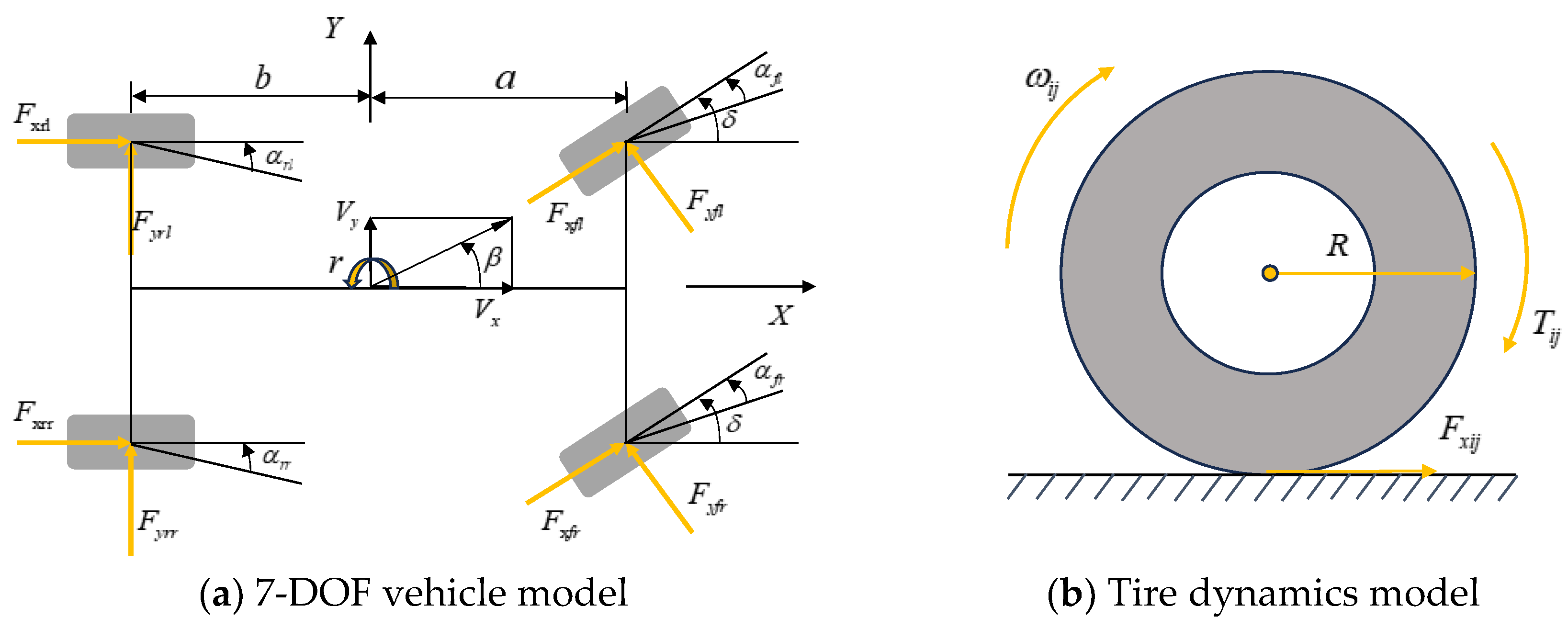
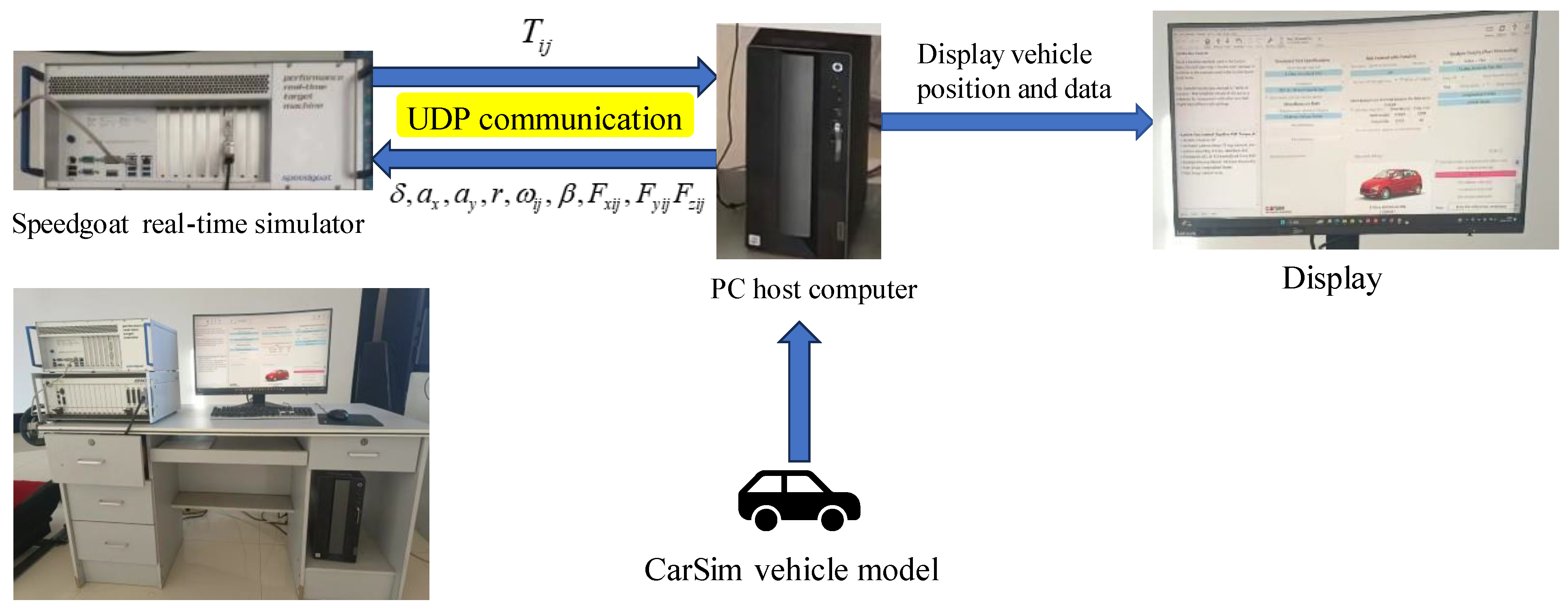
The structure of this paper is as follows: Section 2 presents the 7-DOF and 2-DOF vehicle dynamics models, as well as the tire model, and calculates the desired yaw rate and the sideslip angle. Section 3 introduces the CKF-based road adhesion coefficient estimator, the second-order sliding mode yaw moment controller, and the optimal torque distribution algorithm. Section 4 discusses the construction of the Speedgoat-CarSim hardware-in-the-loop simulation platform and validates the performance of the control algorithms. Finally, Section 5 summarizes the research findings of this study.

2. Vehicle Dynamics Model

This section focuses on the establishment of the vehicle dynamics model needed in this paper, including the 2-DOF vehicle model and the 7-DOF vehicle model, of which some variable parameters are shown in

Table 1. Parameters of variables.

Symbol	Description
$m$	Vehicle mass
$\delta$	Steering angle of the front wheel
$\beta$	Vehicle sideslip angle
$V_x,V_y$	Vehicle longitudinal and lateral velocity
$r$	Yaw rate
$I_z$	Inertia moment about the vehicle vertical axis
$a,b$	Distance from vehicle gravity center to front and rear axles, respectively
$F_{xf},F_{xr}$	Total front and rear longitudinal tire forces, respectively
$F_{yf},F_{yr}$	Total front and rear lateral tire forces, respectively
$I_w$	Wheel moment of inertia
$R$	Effective wheel radius
${\omega }_{ij}$	Wheel angular speed of four wheels, respectively
$F_{xij},F_{yij},F_{zij}$	Longitudinal, lateral and vertical tire forces of four wheels, respectively
$T_{ij}$	Driving torques of four wheels, respectively
$B_f,B_r$	Front and rear axle wheelbases, respectively
$h_g$	Center of mass height
${\alpha }_{ij}$	Sideslip angle of four wheels, respectively
$V_{tij}$	Longitudinal speed of each wheel center
${\lambda }_{ij}$	Slip rate of each wheel
$k_f,k_r$	Lateral deflection stiffness of front and rear wheels

.

2.1. Seven-Degree-of-Freedom Vehicle Model

In describing the kinematic characteristics of the vehicle, it is assumed that the vehicle travels on a horizontal road surface and is analyzed with the center of mass of the vehicle as the origin of the body coordinate system. When considering the vertical motion of the vehicle, the suspension system is simplified as a rigid entity and the pitch and roll of the vehicle are not considered. Meanwhile, the effect of longitudinal rolling resistance is ignored when a state parameter estimation is performed. On this basis, a 7-DOF nonlinear whole-vehicle model is constructed, as shown in Figure 1. In this model, the X-axis represents the longitudinal direction of the car, and the Y-axis represents the lateral direction of the car; all the directions about angles and in-plane moments are defined as positive with a counterclockwise rotation; all the vector components are taken as positive when they are in the same direction as the coordinate axes.

The dynamic equation of the vehicle’s 7-DOF model was derived based on Figure 1a. The equation for the longitudinal force equilibrium is as follows:

$$m({\dot{V}}_x-r\cdot V_y)=(F_{xfl}+F_{xfr})\cos \delta -(F_{yfl}+F_{yfr})\sin \delta +F_{xrl}+F_{xrr}$$

(1)

The equation governing the lateral dynamics can be expressed as follows:

$$m({\dot{V}}_y+r{V}_x)=(F_{xfl}+F_{xfr})\sin \delta +(F_{yfl}+F_{yfr})\cos \delta +F_{yrl}+F_{yrr}$$

(2)

The equation for torque equilibrium around the Z-axis is given as

$$\begin{array}{l}{I}_z\dot{r}=[(F_{xfl}+F_{xfr})\sin \delta +(F_{yfl}+F_{yfr})\cos \delta ]a+[(F_{xfr}-F_{xfl})\cos \delta \\ \begin{array}{cc}& \end{array}+(F_{yfl}-F_{yfr})\sin \delta ]{\displaystyle \frac{B_f}{2}}+(F_{xrr}-F_{xrl}){\displaystyle \frac{B_r}{2}}-(F_{yrl}+F_{yrr})b\end{array}$$

(3)

The equation for the torque balance across all four wheels is expressed as

$$I_w{\dot{\omega }}_{ij}=-R{F}_{xij}+T_{ij}$$

(4)

The equation for the vertical load on each tire is presented as

$$F_{z\_fl,fr}=mg{\displaystyle \frac{b}{2l}}-m{\dot{V}}_x{\displaystyle \frac{h_g}{2l}}\pm m{\dot{V}}_y{\displaystyle \frac{h_g}{B_f}}{\displaystyle \frac{b}{l}},F_{z\_rl,rr}=mg{\displaystyle \frac{a}{2l}}+m{\dot{V}}_x{\displaystyle \frac{h_g}{2l}}\mp m{\dot{V}}_y{\displaystyle \frac{h_g}{B_r}}{\displaystyle \frac{a}{l}}$$

(5)

2.2. Two-Degree-of-Freedom Vehicle Model

As shown in Figure 2, the 2-DOF vehicle model reflects the response characteristics of the vehicle in the linear region, which is a more familiar form of vehicle performance for most drivers. Therefore, the calculation of desired control parameters based on this model can help to improve the driver’s sense of discomfort in the face of the vehicle’s nonlinear region maneuvering characteristics and effectively reduce the difficulty of control. In this paper, a 2-DOF vehicle model is used to obtain the desired swing angular velocity of the vehicle, which is used as the basis for further control design and analysis.

$$\left\{\begin{array}{l}m{\dot{V}}_y=F_{yf}\cos \delta +F_{yr}+F_{xf}\sin \delta \\ I_z\dot{r}=(F_{yf}\cos \delta +F_{xf}\sin \delta )a-F_{yr}b\end{array}\right.$$

(6)

The 2-DOF vehicle model has only two degrees of freedom, transverse and lateral, and is the most basic model for studying the maneuvering stability of the whole vehicle. Based on the derivation from Equation (6), the differential equation of motion can be expressed as

$$\left\{\begin{array}{l}\dot{\beta }={\displaystyle \frac{k_f+k_r}{m{V}_x}}\beta +({\displaystyle \frac{a{k}_f-b{k}_r}{m{V}_x^2}}-1)r-{\displaystyle \frac{k_f}{m{V}_x}}\delta \\ \dot{r}={\displaystyle \frac{a{k}_f-b{k}_r}{I_z}}\beta +{\displaystyle \frac{a^2{k}_f+b^2{k}_r}{I_z{V}_x}}r-{\displaystyle \frac{a{k}_f}{I_z}}\delta \end{array}\right.$$

(7)

The independent variable in this equation is time. When the vehicle is in a steady state, both $\dot{\beta }$ and $\dot{r}$ are zero and the desired yaw rate and sideslip angle can be derived as follows:

$$r_d={\displaystyle \frac{V_x}{L(1+K{V}_x^2)}}\delta ,{\beta }_d={\displaystyle \frac{a/L+mb{V}_x^2/(L^2{k}_r)}{1+K{V}_x^2}}\delta$$

(8)

where $L$ is the axial distance and $K$ is the stability factor. $K={\displaystyle \frac{\mathrm{m}}{L^2}}({\displaystyle \frac{a}{k_r}}-{\displaystyle \frac{b}{k_f}})$.

Due to the limitation of the ground attachment limit, the desired angular velocity of the pendulum needs to satisfy

$$\left|r_{\max }\right|=\theta {\displaystyle \frac{\mu \mathrm{g}}{V_x}}$$

(9)

where $\theta$ is the safety factor, generally taken as 0.85, and $g$ the gravitational acceleration, taken as 9.8.

Therefore, the final desired angular velocity of the pendulum is taken as

$$r_d=\min \{\left|{\displaystyle \frac{V_x}{L(1+K{V}_x^2)}}\delta \right|,\left|r_{\max }\right|\}\cdot \mathrm{sgn}(\delta )$$

(10)

The desired sideslip angle is to be defined as

$$\begin{array}{l}{\beta }_d={\displaystyle \frac{b/L+ma{V}_x^2/(L^2{k}_r)}{1+K{V}_x^2}}\delta ={\displaystyle \frac{V_x^2/L}{1+K{V}_x^2}}\delta ({\displaystyle \frac{b}{V_x^2}}+{\displaystyle \frac{ma}{k_{r}L}})=r_{\exp }{V}_x({\displaystyle \frac{b}{V_x^2}}+{\displaystyle \frac{ma}{k_{r}L}})\\ \end{array}$$

(11)

The sideslip angle is limited to

$$\left|{\beta }_{\max }\right|=\mu \mathrm{g}({\displaystyle \frac{b}{V_x^2}}+{\displaystyle \frac{ma}{k_{r}L}})$$

(12)

Therefore, the final desired sideslip angle is taken as

$$\begin{array}{l}{\beta }_d=\min \{\left|{\displaystyle \frac{b/L+m{L}_f{V}_x^2/(L^2{k}_r)}{1+K{V}_x^2}}\delta \right|,\left|{\beta }_{\max }\right|\}\cdot \mathrm{sgn}({\displaystyle \frac{b/L+ma{V}_x^2/(L^2{k}_r)}{1+K{V}_x^2}}\delta )\\ \end{array}$$

(13)

2.3. Magic Formula Tire Model

In this section, the magic formula tire model [24] is selected for vehicle dynamics analysis. The model fits the experimental data of tires through a combination of trigonometric equations which accurately describe the relationship between the longitudinal force, lateral force and correction moment and the tire slip rate, lateral deflection angle, vertical load, and adhesion coefficient. The magic formula has a high fitting accuracy and can effectively reflect the nonlinear characteristics of tires under different working conditions. Its unified expression is as follows:

$$y(x)=\mu D\sin (C\arctan \left\{Bx-E(Bx-\arctan (Bx))\right\})$$

(14)

$$Y(x)=y(x)+S_v$$

(15)

$$x=X+S_h$$

(16)

where $Y$ can be expressed as lateral force, longitudinal force, etc., $x$ is an input variable which can be the slip rate, lateral deflection angle, or camber angle, $B$ is the stiffness factor, $C$ is the shape factor of the curve, $D$ is the peak factor, $E$ is the curvature factor of the curve, $S_v$ is the amount of drift in the horizontal direction, and $S_h$ is the amount of drift in the vertical direction.

Equation (14) can be calculated through the pure slip or pure lateral bias conditions of the tire longitudinal force $F_{xij0}$ and lateral force $F_{yij0}$; however, in the actual operation of the vehicle, the tire slip and lateral bias often occurs at the same time. At this time, the tire longitudinal and lateral force there is a coupling. This condition is known as a joint conditions; the joint conditions associated with the longitudinal and lateral forces of the tire are defined as:

$$F_{xij}={\displaystyle \frac{{\sigma }_x}{\sqrt{{\sigma }_x^2+{\sigma }_y^2}}}{F}_{xij0},F_{yij}={\displaystyle \frac{{\sigma }_y}{\sqrt{{\sigma }_x^2+{\sigma }_y^2}}}{F}_{yij0}$$

(17)

where ${\sigma }_x=-{\displaystyle \frac{{\lambda }_{ij}}{1+{\lambda }_{ij}}},{\sigma }_y={\displaystyle \frac{\tan {\alpha }_{ij}}{1+{\lambda }_{ij}}}$.

3. Stability Control Algorithm

In the previous section, the establishment of the vehicle model and the calculation of the desired yaw rate and the desired sideslip angle have been introduced. This section will focus on the design of the roadway adhesion coefficient estimator, the transverse pendulum moment controller and the optimal moment distributor. The functions of each part and the overall algorithm flow are shown in Figure 3. The vehicle model first outputs the state information of the vehicle, based on which the observation layer performs the computation of the desired yaw rate and the desired sideslip angle, and estimates the road surface attachment coefficient using the improved CKF algorithm. Subsequently, the yaw moment control layer calculates the variable error based on the estimated road surface attachment coefficient and performs tracking control, finally achieving torque allocation for the optimal loading rate of each tire by jointly allocating the driving torque.

3.1. CKF Road Adhesion Coefficient Estimation Algorithm

In this paper, a CKF algorithm is introduced to improve the stability and accuracy of state estimation based on the standard CKF with singular value decomposition to optimize the error covariance matrix.

Initially, a nonlinear system is formulated using the following state and volume equations:

$$\left\{\begin{array}{l}{\dot{X}}_p=f(X_p,U_k),\\ Z_p=h(X_p,U_k).\end{array}\right.$$

(18)

where the control input $U_k$ includes the front-wheel angle, the driving forces applied to the four wheels, along with the transverse and longitudinal forces acting on the tires, namely, $U_k=[\delta ,T_{dij},F_{xij},F_{yij}]$, while $X_p$ represents the adhesion coefficient, which includes the road adhesion coefficient for each wheel, namely, $X_p=[{\mu }_{fl},{\mu }_{fr},{\mu }_{rl},{\mu }_{rr}]$. In this system, the measured outputs are the longitudinal acceleration, lateral acceleration, and yaw rate, all of which can be easily measured by the sensors, namely, $Z_p=[a_x,a_y,r]$.

Step 1: Time update of the adhesion coefficient variable

(1)

The error covariance matrix $P_{p,k-1}$ is optimized through singular value decomposition.

$$P_{p,k-1}=A_{p,k-1}{\Lambda }_{p,k-1}{A}_{p,k-1}^T$$

(19)

The columns of $A_{p,k-1}$ are the unit orthogonal eigenvectors of the error covariance matrix $P_{p,k-1}$,${\Lambda }_{p,k-1}$ is a diagonal matrix, and ${\Lambda }_{p,k-1}=diag[S_{p1}^2,S_{p2}^2\dots \dots S_{pn}^2]$, where $S_{pi}$ is the eigenvalue of $P_{p,k-1}$.

$$X_{pj,k-1}=A_{pj,k-1}{S}_{pi}{\xi }_{pj}+X_{p,k-1}^{\wedge }$$

(20)

$$\left\{\begin{array}{l}{\xi }_{pj}=\sqrt{{\displaystyle \frac{d}{2}}}{[1]}_{pj}\\ d=2n(\mathrm{Third}-\mathrm{order} \mathrm{cubature} \mathrm{criterion})\end{array}\right.$$

(21)

where ${\xi }_{pj}$ is the cubature point, ${[1]}_{pj}$ represents the j-th element in the cubature point set, $d$ is the total number of cubature points, and $n$ is the state vector. In the adhesion coefficient variable, $n=4$, the collection of cubature points is shown below.

$$\left\{\left[\begin{array}{l}1\\ 0\\ 0\\ 0\end{array}\right]\right.\left|\left[\begin{array}{l}0\\ 1\\ 0\\ 0\end{array}\right]\right|\left[\begin{array}{l}0\\ 0\\ 1\\ 0\end{array}\right]\left|\left[\begin{array}{l}0\\ 0\\ 0\\ 1\end{array}\right]\right|\left[\begin{array}{l}-1\\ 0\\ 0\\ 0\end{array}\right]\left|\left[\begin{array}{l}0\\ -1\\ 0\\ 0\end{array}\right]\right|\left[\begin{array}{l}0\\ 0\\ -1\\ 0\end{array}\right]|\left.\left[\begin{array}{l}0\\ 0\\ 0\\ -1\end{array}\right]\right\}$$

(2)

Cubature point $X_{pj,k/k-1}^{*}$ is calculated as

$$X_{pj,k/k-1}^{*}=f(X_{pj,k/k-1})$$

(22)

(3)

The predicted value of the variable $X_{p,k/k-1}^{\wedge }$ is derived as

$$X_{p,k/k-1}^{\wedge }={\displaystyle \sum _{j=1}^d\frac{1}{d}{X}_{pj,k/k-1}^{*}}$$

(23)

(4)

The covariance predicted value $P_{p,k/k-1}$ is obtained as

$$P_{p,k/k-1}={\displaystyle \sum _{j=1}^d\frac{1}{d}{X}_{pj,k/k-1}^{*}}{X}_{pj,k/k-1}^{*T}-X_{p,k/k-1}^{\wedge }{X}_{p,k/k-1}^{\wedge T}+Q_p$$

(24)

where $Q_p$ is the process noise covariance.

Step 2: Measurement update of the adhesion coefficient variable $X_p$

(1)

The error covariance matrix $P_{p,k/k-1}$ is optimized by singular value decomposition.

$$\left\{\begin{array}{l}{P}_{p,k/k-1}=A_{p,k/k-1}{\Lambda }_{p,k/k-1}{A}_{p,k/k-1}^T\\ X_{pj,k/k-1}=A_{pj,k/k-1}{S}_{pi,k/k-1}{\xi }_{pj}+X_{p,k/k-1}^{\wedge }\end{array}\right.$$

(25)

(2)

The new cubature point $Z_{pj,k/k-1}$ is derived as

$$Z_{pj,k/k-1}=h(X_{pj,k/k-1},X_{sj,k/k-1}^{\wedge },U_k)$$

(26)

(3)

The average cubature point $Z_{p,k/k-1}^{\wedge }$ is obtained as

$$Z_{p,k/k-1}^{\wedge }={\displaystyle \sum _{j=1}^d\frac{1}{d}}{Z}_{pj,k/k-1}$$

(27)

(4)

The information covariance matrix $P_{pzz,k/k-1}$ is given as

$$P_{pzz,k/k-1}={\displaystyle \sum _{j=1}^d\frac{1}{d}}{Z}_{pj,k/k-1}{Z}_{pj,k/k-1}^T-Z_{p,k/k-1}^{\wedge }{Z}_{p,k/k-1}^{\wedge T}+R_p$$

(28)

where $R_p$ is the measurement noise covariance.

(5)

The cross-covariance matrix $P_{pxz,k/k-1}$ is calculated as

$$P_{pxz,k/k-1}={\displaystyle \sum _{j=1}^d\frac{1}{d}}{X}_{pj,k/k-1}{Z}_{pj,k/k-1}^T-X_{p,k/k-1}^{\wedge }{Z}_{p,k/k-1}^{\wedge T}$$

(29)

(6)

The gain matrix $K_{pk}$ is derived as

$$K_{pk}=P_{pxz,k/k-1}{P}_{pzz,k/k-1}^{-1}$$

(30)

(7)

The measured parameter variable $X_{p,k}^{^}$ is obtained by

$$X_{p,k}^{^}=X_{p,k/k-1}^{^}+K_{pk}(Z_p{,}_k{Z}_{p,k/k-1}^{^})$$

(31)

(8)

The error covariance matrix after measurement $P_{p,k}$ is derived as

$$P_{p,k}=P_{p,k/k-1}-K_{pk}{P}_{pzz,k/k-1}{K}_{pk}^T$$

(32)

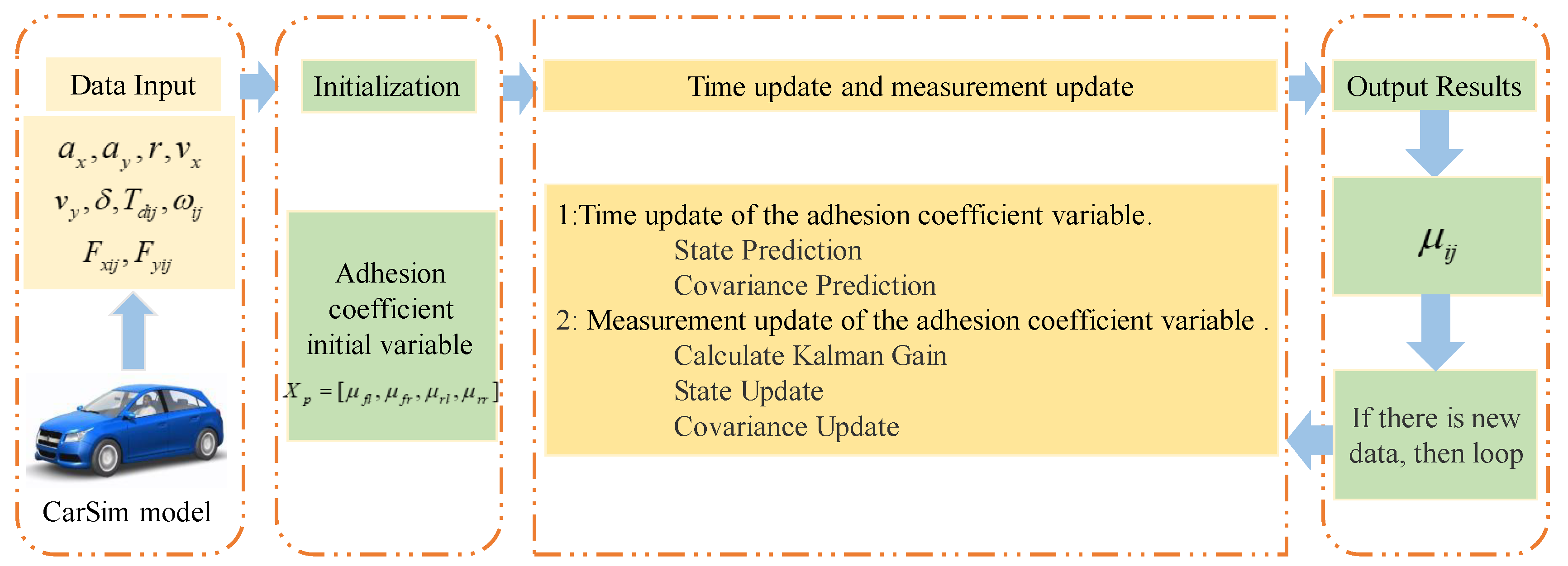
The specific algorithm flow is shown in Figure 4.

3.2. Second-Order Sliding Mode Control Algorithm

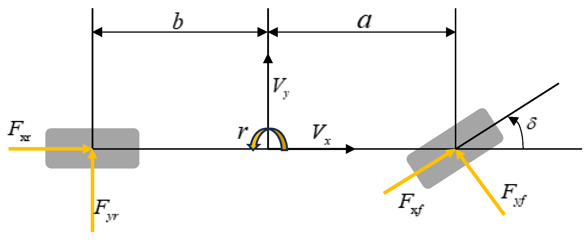
The core objective of the transverse yaw moment decision-making is to make the yaw rate follows its desired value as much as possible under the premise of ensuring a small sideslip angle so as to effectively meet the driver’s driving intention. Therefore, based on the 2-DOF vehicle model, this paper selects the transverse pendulum angular velocity and its rate of change and the sideslip angle and its rate of change as the control variables and comprehensively considers the coupling relationship between the two, designing the weighted control module to make decisions on the additional transverse pendulum moments so as to ensure the stability of the vehicle. To this end, the second-order sliding mode control algorithm is used in this section to track the yaw rate and the sideslip angle and calculate the corresponding additional traverse moments. The differential equations of the original 2-DOF model can be rewritten as

$$\left\{\begin{array}{l}\dot{\beta }={\displaystyle \frac{k_f+k_r}{m{V}_x}}\beta +({\displaystyle \frac{a{k}_f-b{k}_r}{m{V}_x^2}}-1)r-{\displaystyle \frac{k_f}{m{V}_x}}\delta \\ \dot{r}={\displaystyle \frac{a{k}_f-b{k}_r}{I_z}}\beta +{\displaystyle \frac{a^2{k}_f+b^2{k}_r}{I_z{V}_x}}r-{\displaystyle \frac{a{k}_f}{I_z}}\delta +{\displaystyle \frac{\Delta M}{I_{\mathrm{z}}}}\end{array}\right.$$

(33)

where $\Delta M$ is the additional pendulum moment.

3.2.1. Yaw Rate Control

When following the yaw rate control, define the yaw rate tracking error and its error rate of change as follows:

$$\begin{array}{l}{e}_r=r-r_d\\ {\dot{e}}_r=\dot{r}-{\dot{r}}_d\end{array}$$

(34)

The sliding mold surface is defined as

$$s_r=c_1{e}_r+c_2{\dot{e}}_r$$

(35)

where $s_r$ is the slip mode variable defined based on the yaw rate and $c_1,c_2$ are the yaw rate deviation coefficient and the yaw rate change rate deviation coefficient. The slip mode of convergence is selected as the exponential convergence law. That is ${\dot{\mathrm{s}}}_r=-{\epsilon }_{1}s-k_{1}sgn\left(s\right)$.

It is calculated that:

$$\begin{array}{ll}{\dot{s}}_r& =c_1{\dot{e}}_r+c_2{\ddot{e}}_r\\ & =c_2[{\displaystyle \frac{a{k}_f-b{k}_r}{I_z}}\dot{\beta }+({\displaystyle \frac{a^2{k}_f+b^2{k}_r}{I_z{V}_x}}+c_1)\dot{r}-{\displaystyle \frac{a{k}_f}{I_z}}\dot{\delta }-{\displaystyle \frac{c_1}{c_2}}{\dot{r}}_d-{\ddot{r}}_d]+{\displaystyle \frac{\Delta {\dot{M}}_r}{I_z}}\\ & =X+{\displaystyle \frac{\Delta {\dot{M}}_r}{I_z}}\end{array}$$

(36)

The additional pendulum moment is deduced to be:

$$\Delta M_r={\displaystyle \int (-I_z[{\epsilon }_{1}s-k_{1}sgn\left(s\right)+X])dt}$$

(37)

3.2.2. Sideslip Angle Control

When controlling based on the sideslip angle, the sideslip angle tracking error and its rate of change are defined as follows:

$$\begin{array}{l}{e}_{\beta }=\beta -{\beta }_d\\ {\dot{e}}_{\beta }=\dot{\beta }-{\dot{\beta }}_d\end{array}$$

(38)

The sliding mold surface is defined as

$$s_{\beta }=c_3{e}_{\beta }+c_4{\dot{e}}_{\beta }$$

(39)

where $s_{\beta }$ is the sliding mode variable defined based on the sideslip angle and $c_3,c_4$ are the sideslip angle deviation coefficients and the sideslip angle change rate deviation coefficients. The exponential convergence law is chosen for the sliding mode convergence algorithm, i.e., ${\dot{\mathrm{s}}}_{\beta }=-{\epsilon }_{2}s-k_{2}sgn\left(s\right)$.

It is calculated that

$$\begin{array}{l}{s}_{\beta }=c_3{\dot{e}}_{\beta }+c_4{\ddot{e}}_{\beta }=c_4\{({\displaystyle \frac{k_f+k_r}{m{V}_x}}+c_3)[{\displaystyle \frac{k_f+k_r}{m{V}_x}}\beta +({\displaystyle \frac{a{k}_f-b{k}_r}{m{V}_x^2}}-1)r-{\displaystyle \frac{k_f}{m{V}_x}}\delta ]\\ \begin{array}{c}\end{array}+({\displaystyle \frac{a{k}_f-b{k}_r}{m{V}_x^2}}-1)({\displaystyle \frac{a{k}_f-b{k}_r}{I_z}}\beta +{\displaystyle \frac{a^2{k}_f+b^2{k}_r}{I_z{V}_x}}r-{\displaystyle \frac{a{k}_f}{I_z}}\delta )-c_3{\dot{\beta }}_d-c_4{\ddot{\beta }}_d\}\\ \begin{array}{c}\end{array}+({\displaystyle \frac{a{k}_f-b{k}_r}{m{V}_x^2}}-1){\displaystyle \frac{\Delta M_{\beta }}{I_z}}\begin{array}{c}=\end{array}Y+({\displaystyle \frac{a{k}_f-b{k}_r}{m{V}_x^2}}-1){\displaystyle \frac{\Delta M_{\beta }}{I_z}}\end{array}$$

(40)

The additional pendulum moment is deduced to be

$$\Delta M_{\beta }=-I_z[-{\epsilon }_{2}s-k_{2}sgn\left(s\right)+Y]{(1-{\displaystyle \frac{a{k}_f-b{k}_r}{m{V}_x^2}})}^{-1}$$

(41)

3.3. Joint Distribution Module

At present, there are many methods for determining vehicle instability, and Wang [25] analyzes and summarizes many methods and gives the vehicle instability criteria. The critical value of destabilization and the boundary parameter of phase plane stability for the deviation of yaw rate and phase plane stability of an ordinary B-type vehicle are shown in

Table 2. Critical values of destabilization zone of yaw rate deviation ($\kappa$).

Speed (km/h)	Critical Value of Instability Zone of Yaw Rate Deviation (rad/s)
60	0.025
70	0.026
80	0.027
90	0.028
100	0.03
120	0.03

and

Table 3. Phase plane stability parameters.

Road Adhesion Coefficient	${\mathit{B}}_1$	${\mathit{B}}_2$
$0.8\le \mu \le 1$	0.357	5.573
$0.6\le \mu \le 0.8$	0.357	4.654
$0.4\le \mu \le 0.6$	0.303	4.228
$0.2\le \mu \le 0.4$	0.297	3.345
$\mu <0.2$	0.284	2.577

.

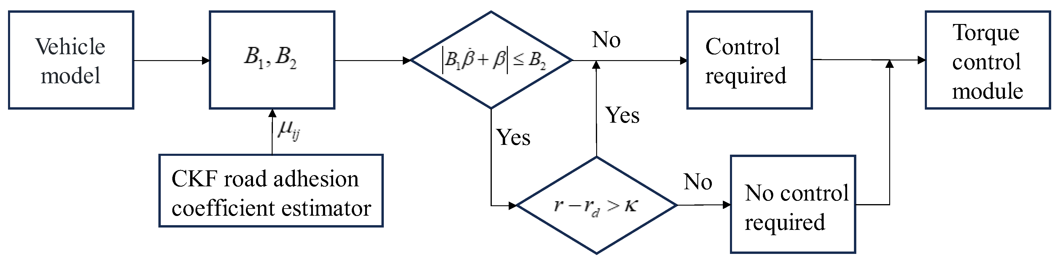
Which satisfies $\left|B_1\dot{\beta }+\beta \right|\le B_2$, as the vehicle is stable and controllable. The specific allocation logic is shown in Figure 5: the vehicle is destabilized by the phase plane stability parameter; if it does not satisfy $\left|B_1\dot{\beta }+\beta \right|\le B_2$, then the vehicle is destabilized and the sideslip angle following control is selected to output the additional transverse moment, and if the vehicle is not destabilized, the joint yaw angular velocity following and sideslip angle following output the additional transverse moment in accordance with a certain allocation ratio.

The specific allocation algorithm is linear and the allocation ratio is given in the following formula:

$$p=\left\{\begin{array}{cc}0& {\displaystyle \frac{\left|B_1\dot{\beta }+\beta \right|}{B_2}}=0\\ {\displaystyle \frac{\left|B_1\dot{\beta }+\beta \right|}{B_2}}& 0<{\displaystyle \frac{\left|B_1\dot{\beta }+\beta \right|}{B_2}}<1\\ 1& {\displaystyle \frac{\left|B_1\dot{\beta }+\beta \right|}{B_2}}\ge 1\end{array}\right.$$

(42)

The joint allocation expression is as follows:

$$\Delta M=p\Delta M_r+(1-p)\Delta M_{\beta }$$

(43)

3.4. Optimal Distribution of Torque

In the previous paper, the yaw rate and the sideslip angle are selected as the control parameters and the second-order sliding mode control algorithm is used to regulate them, so as to make the yaw rate follow the desired value; also, the additional yaw moment required to maintain the stability of the vehicle is solved. The task at the lower level is to distribute the calculated additional yaw moment to the four wheels’ hub motors, based on the optimal tire load distribution, to ensure stable vehicle operation. The vehicle is in contact with the ground through the tires, but the tires have a force limit, i.e., increasing the longitudinal force will lead to a decrease in the lateral force. Therefore, the objective of optimal torque distribution in this layer is to reasonably distribute the longitudinal driving force to reduce the loading rate of each tire, thereby ensuring a large lateral force margin for the tires and effectively improving the lateral stability of the vehicle.

The objective function is defined as

$$\min J=\min \Sigma {\displaystyle \frac{F_{xij}^2+F_{yij}^2}{{\left({\mu }_{ij}{F}_{zij}\right)}^2}}$$

(44)

Since the drive motor can only control the longitudinal force, this simplifies to

$$\min J=\min \Sigma {\displaystyle \frac{F_{xij}^2}{{\left({\mu }_{ij}{F}_{zij}\right)}^2}}$$

(45)

Bringing in $F_{xij}={\displaystyle \frac{T_{ij}}{R}}$, the final objective function is

$$\min J=\min \Sigma {\displaystyle \frac{T_{ij}^2}{{\left({\mu }_{ij}{F}_{zij}R\right)}^2}}$$

(46)

The total driving moment $T$ and the additional yaw moment $\Delta M$ are related as follows:

$$\begin{array}{l}(T_{fl}+T_{fr})\cos \delta +T_{rl}+T_{rr}=T\\ {\displaystyle \frac{B_f}{2R}}(-T_{fl}+T_{fr})\cos \delta -{\displaystyle \frac{B_r}{2R}}{T}_{rl}+{\displaystyle \frac{B_r}{2R}}{T}_{rr}=\Delta M\end{array}$$

(47)

The optimization problem designed in this paper has only two equation constraints, but there are four independent variables, and solving it by using the equation constraints brought into the objective function can greatly improve the computational efficiency. As the general vehicle front and rear wheelbase approximation then make $B_f=B_r=B_l$, Equation (47) can be changed t:

$$T_{fl}=({\displaystyle \frac{T}{2}}-{\displaystyle \frac{\Delta M}{B_l}}R-T_{rl}){\displaystyle \frac{1}{\cos \delta }},T_{fr}=({\displaystyle \frac{T}{2}}+{\displaystyle \frac{\Delta M}{B_l}}R-T_{rr}){\displaystyle \frac{1}{\cos \delta }}$$

(48)

Equation (48) is carried into Equation (46) to obtain

$$\begin{array}{l}J={\displaystyle \frac{{[\frac{1}{\cos \delta }(\frac{T}{2}-\frac{\Delta M}{B_l}R-T_{rl})]}^2}{{\left({\mu }_{fl}{F}_{zfl}R\right)}^2}}+{\displaystyle \frac{{[\frac{1}{\cos \delta }(\frac{T}{2}+\frac{\Delta M}{B_l}R-T_{rr})]}^2}{{\left({\mu }_{fr}{F}_{zfr}R\right)}^2}}\\ \begin{array}{c}\end{array}+{\displaystyle \frac{T_{rl}^2}{{\left({\mu }_{rl}{F}_{zrl}R\right)}^2}}+{\displaystyle \frac{T_{rr}^2}{{\left({\mu }_{rr}{F}_{zrr}R\right)}^2}}\end{array}$$

(49)

Equation (49) takes partial derivatives with respect to $T_{rl}$ and $T_{rr}$:

$$\begin{array}{l}{\displaystyle \frac{\partial J}{\partial T_{rl}}}=-{\displaystyle \frac{2\left(\frac{T}{2}-\frac{\Delta M}{B_l}R-T_{rl}\right)}{{\left(\cos \delta {\mu }_{fl}{F}_{zfl}R\right)}^2}}+{\displaystyle \frac{2T_{rl}}{{\left({\mu }_{rl}{F}_{zrl}R\right)}^2}}\\ {\displaystyle \frac{\partial J}{\partial T_{rr}}}=-{\displaystyle \frac{2\left(\frac{T}{2}+\frac{\Delta M}{B_l}R-T_{rr}\right)}{{\left(\cos \delta {\mu }_{fr}{F}_{zfr}R\right)}^2}}+{\displaystyle \frac{2T_{rr}}{{\left({\mu }_{rr}{F}_{zrr}R\right)}^2}}\end{array}$$

(50)

Let Equation (50) be zero, then the minimum value can be found with

$$T_{rl}={\displaystyle \frac{\frac{{\mu }_{rl}^2{F}_{zrl}^{2}T}{2}-\frac{{\mu }_{rl}^2{F}_{zrl}^2\Delta M}{B_l}R}{{\mu }_{rl}^2{F}_{zrl}^2+{\mu }_{fl}^2{F}_{zfl}^2\cos \delta }},T_{rr}={\displaystyle \frac{\frac{{\mu }_{rr}^2{F}_{zrr}^{2}T}{2}+\frac{{\mu }_{rr}^2{F}_{zrr}^2\Delta M}{B_l}R}{{\mu }_{rr}^2{F}_{zrr}^2+{\mu }_{fr}^2{F}_{zfr}^2\cos \delta }}$$

(51)

Equation (51) can be substituted into Equation (48) to find $T_{fl},T_{fr}$.

4. Hardware-in-the-Loop Experimental Verification

4.1. Hardware-in-the-Loop Platform

The hardware-in-the-loop simulation platform is shown in Figure 6 and consists of the host computer, Speedgoat simulation machine, the data collector, and the driving simulator. A stability control strategy was developed in MATLAB/Simulink, compiled into code, and downloaded to a Speedgoat real-time target machine. The Speedgoat system was then interfaced with CarSim for co-simulation, where the CarSim vehicle dynamics model was executed on the host machine and the stability control program was executed on the Speedgoat system. The Speedgoat machine received real-time vehicle signals and computed wheel torques. The specific configurations are as follows: The host machine is equipped with an Intel i7-10700 processor (Intel (China) Co., Ltd., China), an RTX 3060 graphics card and 64 GB of RAM. The Speedgoat system features an Intel i3 processor (Intel (China) Co., Ltd., China) with 4 GB of RAM. The driving suite utilizes a Logitech G27 (Logitech Technologies (Suzhou) Co., Ltd., Suzhou, China). Some of the parameters of the vehicle model are set as shown in

Table 4. Vehicle parameters.

Parameter	Value	Parameter	Value
$m(kg)$	1412	$h_g(m)$	0.54
$I_z(kg\cdot m^2)$	1536.7	$R(m)$	0.32
$a(m)$	1.01	$P_n(kW)$	68
$b(m)$	1.89	$T_n(N\cdot m)$	140
$I_w(kg\cdot m^2)$	0.9

where $P_n$ is the rated power of each motor and $T_n$ is the rated torque of each motor.

.

The Speedgoat-CarSim simulation platform enables real-time simulation of vehicle dynamics in a virtual environment, with the capability to interact with actual hardware interfaces in later stages. This allows for high-fidelity testing of control algorithms while considering feedback from the real hardware, ensuring the accuracy and reliability of algorithm validation.

The model is based on the assumption of a flat road surface for simulation analysis. While deviations may occur under certain conditions, it provides valuable insights and reasonable approximations for vehicle dynamics analysis on standard highways and typical smooth road surfaces. It is recommended to adjust the model parameters based on specific road conditions to better match the actual vehicle dynamics on different terrains.

4.2. Low-Speed and Low-Road Adhesion Coefficient Double-Shifting Line Condition

Select the double shift line condition, simulation set the initial speed of 70 km/h, road adhesion coefficient 0.4, the initial variable of the adhesion coefficient $X_p=[1,1,1,1]$, the process error covariance matrix $Q_p=0.1\times eye(4)$, the measurement error covariance matrix $R_p=0.01\times eye(3)$; the front-wheel angle signal, the simulation results are shown in Figure 7 and Figure 8 and

Table 5. Algorithm errors on low-adhesion roads.

Parameter	CKF	EKF	UKF
Convergence error of road adhesion coefficient	0.003	0.006	0.004
Convergence speed of road adhesion coefficient	0.7 s	1 s	0.9 s
RMSE	0.3582	0.6224	0.04021
MAE	0.00976	0.03679	0.01372

.

As shown in Figure 7 and Table 5, the CKF road surface adhesion coefficient estimator provides fast and accurate estimates. The CKF converges with an average time of 0.7 s and a post-convergence error of approximately 0.003, outperforming EKF and UKF in both speed and accuracy. While CKF performs well in steady environments, it may face challenges in high-dynamic scenarios, especially when noise is high or the system model is incomplete. Regarding vehicle stability, in the uncontrolled state, the vehicle destabilized in the fourth second and could not remain stable; meanwhile, in the case of average allocation and optimal allocation, the vehicle’s sideslip angle and yaw rate tracked well and could converge quickly to ensure that the vehicle was in a stable state. Among them, the optimal allocation algorithm had the smallest deviation, which is better than the average allocation algorithm and showed a more obvious allocation effect.

In terms of tire loading rate, the optimal torque distribution algorithm has a lower maximum and average loading rate compared to the average distribution. The smaller longitudinal loading rate helps to improve the lateral force margin of the tires, which effectively enhances the lateral stability of the vehicle. This result also verifies that the optimal allocation in Figure 7c,d is better than the average allocation strategy in terms of the accuracy of tracking the sideslip angle and yaw rate. In terms of wheel torque allocation, the four wheels have the same torque in the no-control case; under the average allocation strategy, the torques of the wheels on the same side are equal, while, under the optimal allocation control strategy, the vehicle allocates different torques to different wheels according to the changes in the road conditions, and there are differences in the torque allocation of the wheels on both sides. Especially in cases of oversteer, the optimal torque distribution effectively ensures the stable driving of the vehicle by utilizing the difference in wheel torque to generate additional swing torque under the constraints of wheel output capability and road surface adhesion. In addition, under the optimal torque distribution control strategy, most of the wheel torques are in the driving state, which also ensures the driving dynamics of the vehicle. Although the torque distribution trend of the wheels on the same side is similar, there is a difference in their amplitude and the torque of the front wheels is larger than that of the rear wheels, which reduces the probability of oversteer.

4.3. High-Speed and High-Road Adhesion Coefficient Double-Shifting Line Condition

Select the double shift line condition, simulation set the initial speed of 120 km/h, road adhesion coefficient 0.85, the initial variable of the adhesion coefficient $X_p=[1,1,1,1]$, the process error covariance matrix $Q_p=0.1\times eye(4)$, the measurement error covariance matrix $R_p=0.01\times eye(3)$; the front-wheel angle signal, the simulation results are shown in Figure 9 and Figure 10 and

Table 6. Algorithm errors on high-adhesion roads.

Parameter	CKF	EKF	UKF
Convergence error of road adhesion coefficient	0.001	0.003	0.0012
Convergence speed of road adhesion coefficient	0.4 s	0.75 s	0.7 s
RMSE	0.03274	0.04197	0.03764
MAE	0.00812	0.02438	0.01253

.

As shown in Figure 9 and Table 6, all three algorithms exhibit jitter in estimating the road surface adhesion coefficient. The CKF converges with an average time of 0.4 s and a post-convergence error of 0.001, outperforming EKF and UKF in both convergence speed and accuracy. In terms of vehicle stability, it can be seen that, under high road adhesion coefficient road conditions, the vehicle can be basically stable with or without control; meanwhile, the average and optimal allocation of the vehicle center of mass sideslip angle and yaw rate tracking is better, can be converged quickly, and the control effect is obviously superior to the no-control state, while the optimal allocation algorithm has the smallest deviation and the vehicle stability is the best.

The difference in tire loading rates between the average and optimal distribution algorithms is generally small under high-adhesion conditions. However, when the average distribution algorithm is used, the load rate of the rear wheels of the vehicle is significantly higher than that of the front wheels, which means that the stability of the rear wheels is poorer under this condition. When the vehicle yaw rate is larger, the lateral force margin of the rear wheels is lower, which can easily lead to oversteer and cause vehicle instability. In contrast, the optimal allocation algorithm not only allocates moments to the left and right sides of the vehicle but also optimizes the total moments of the front and rear axles, thus enhancing the overall stability of the vehicle.

To evaluate the computational time of the proposed algorithm in practical applications, a time analysis of the entire control layer was conducted during the simulation. The single computation time of the entire control system is approximately 7.23 ms, which meets the 100 Hz frequency requirement for most real-time control systems. No frame drops were observed in the simulation results, indicating that the Speedgoat processor configuration meets the experimental requirements. Despite significant performance improvements in modern computing platforms, embedded control systems may still face computational resource limitations due to hardware constraints, external environmental variations, and system load.

5. Conclusions

Aiming at the problem of poor maneuvering stability of distributed-drive electric vehicles on high- and low-adhesion road surfaces, this paper proposes a multi-parameter control algorithm based on the estimation of road adhesion coefficients. The specific programs are as follows:

(1) A 7-DOF vehicle dynamics model, as well as a 2-DOF reference model, are established to provide a theoretical basis for the control design.

(2) The higher-level control module calculates the desired yaw rate and sideslip angle based on the 2-DOF vehicle model and estimates the road adhesion coefficient by using the singular-value optimized CKF algorithm. The mid-level control uses a SOSMC as a direct traverse moment controller for tracking the desired yaw rate and sideslip angle. At the same time, the joint distribution algorithm is used for torque distribution in combination with vehicle stability parameters to enhance the robustness of the system. The lower-level control then targets the optimal tire load rate to implement the optimal torque allocation control.

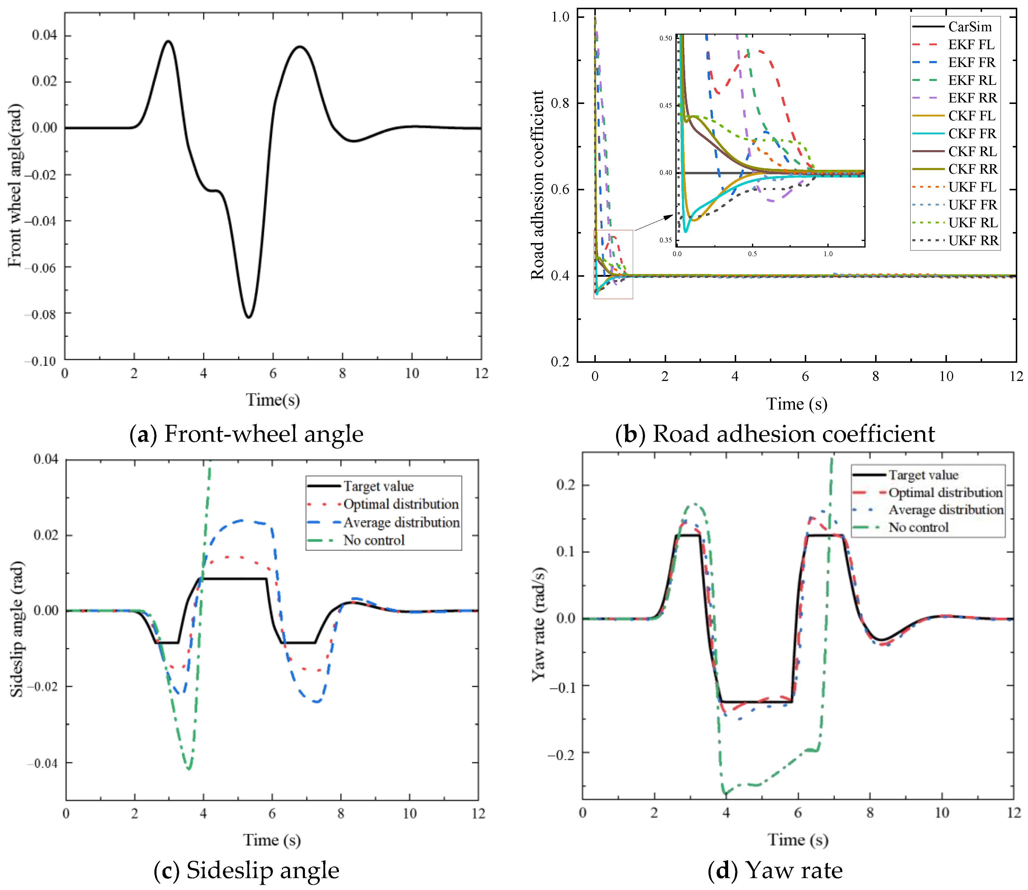
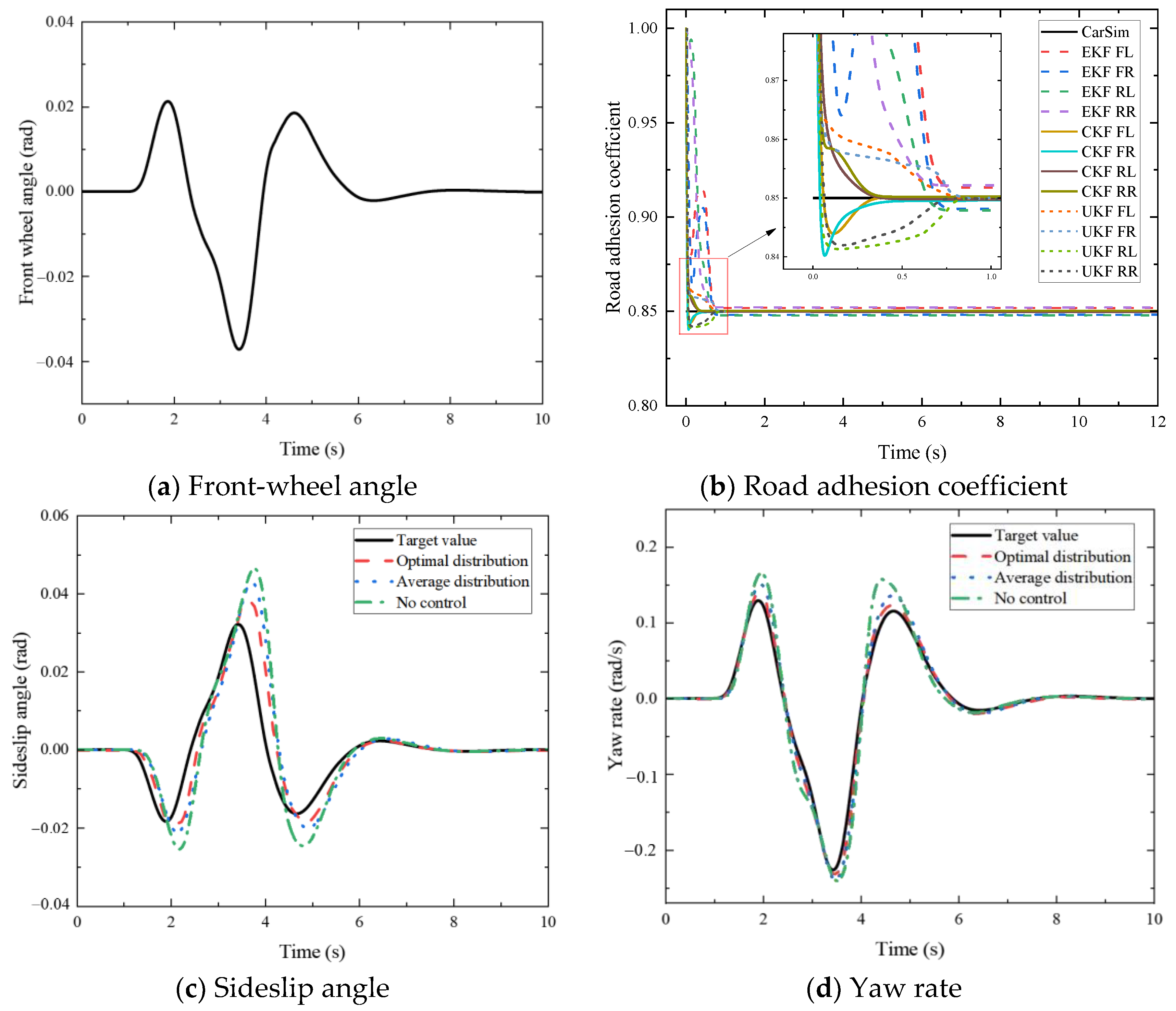
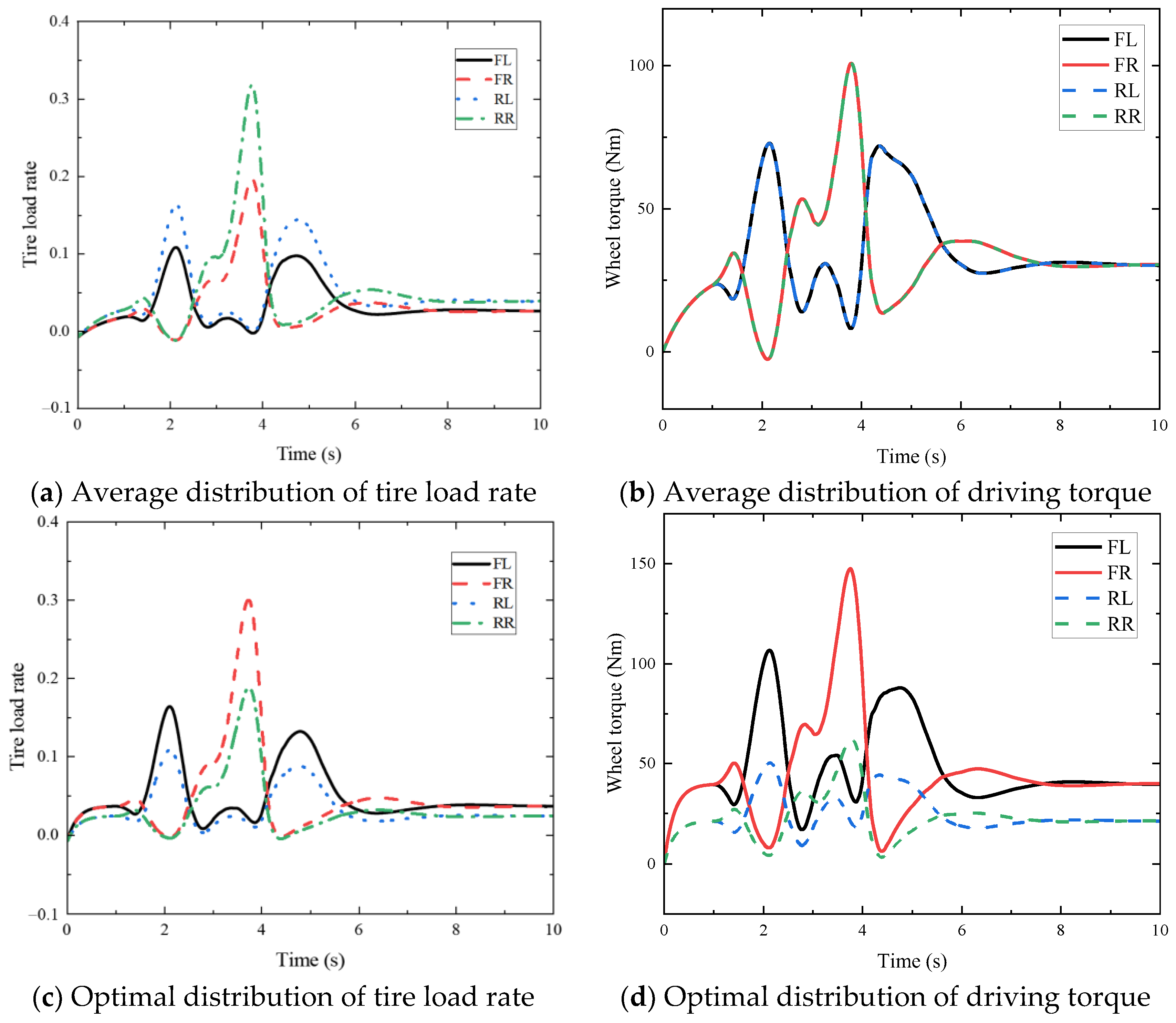
(3) A hardware-in-the-loop simulation platform based on Speedgoat and CarSim is constructed and the stability and accuracy of the proposed control algorithm are verified by setting typical working conditions for testing. The experimental results show that the road adhesion coefficient estimation algorithm can quickly and efficiently estimate the road adhesion coefficient, and its convergence speed is 40% higher than that of the traditional EKF algorithm; additionally, the optimal torque distribution algorithm can reasonably distribute the four-wheel drive force according to the different road adhesion conditions to effectively improve the stability of the vehicle’s maneuvering.

The proposed control method is closely related to vehicle energy efficiency. By accurately estimating the road adhesion coefficient, the system can avoid unnecessary energy waste, particularly on low-traction surfaces or in slip conditions, reducing energy loss caused by excessive driving. The SOSMC helps precisely control the yaw rate, preventing energy waste due to over-correction of the yaw angle. Furthermore, the optimal torque distribution control, based on the optimal tire loading rate, effectively reduces tire slip and energy consumption.

References

1. Chen, H.Y.; Chen, S.P.; Gong, J.W. A Review on the Research of Lateral Control for Intelligent Vehicles. Acta Armamentarii 2017, 38, 1203–1214. [Google Scholar]
2. Zhang, C.; Ma, J.; Chang, B.; Wang, J. Research on Anti-Skid Control Strategy for Four-Wheel Independent Drive Electric Vehicle. World Electr. Veh. J. 2021, 12, 150. [Google Scholar] [CrossRef]
3. Deng, H.F.; Zhao, Y.Q.; Nguyen, T.A.; Huang, C. Fault-Tolerant Predictive Control with Deep-Reinforcement-Learning-Based Torque Distribution for Four In-Wheel Motor Drive Electric Vehicles. IEEE/ASME Trans. Mechatron. 2023, 28, 668–680. [Google Scholar] [CrossRef]
4. Chen, Y.; Yan, H.; Li, Y. Vehicle State Estimation Based on Sage–Husa Adaptive Unscented Kalman Filtering. World Electr. Veh. J. 2023, 14, 167. [Google Scholar] [CrossRef]
5. Zhang, Z.; Yu, J.; Huang, C.; Du, R. Coordinated torque distribution method of distributed drive electric vehicle to reduce control intervention sense. Veh. Syst. Dyn. 2023, 62, 198–221. [Google Scholar] [CrossRef]
6. Liu, Y.; Cui, D.; Peng, W. Vehicle state and parameter estimation based on adaptive anti-outlier unscented Kalman filter and GA-BPNN method. J. Vibroengineering 2024, 26, 139–151. [Google Scholar] [CrossRef]
7. Wu, Y.; Li, G.; Fan, D. Joint estimation of driving state and road adhesion coefficient for distributed drive electric vehicle. IEEE Access 2021, 9, 75460–75469. [Google Scholar] [CrossRef]
8. Wu, Y.F. Estimation of Vehicle State and Road Adhesion Coefficient of Four-Wheel Independent Drive Electric Vehicle. Master’s Thesis, Jilin University, Changchun, China, 2020. [Google Scholar] [CrossRef]
9. Li, S.; Wang, G.; Yang, Z.; Wang, X. Dynamic joint estimation of vehicle sideslip angle and road adhesion coefficient based on DRBF-EKF algorithm. Chin. J. Theor. Appl. Mech. 2022, 54, 1853–1865. [Google Scholar] [CrossRef]
10. Wu, Z.C. Research on the Algorithm of the Road Friction Coefficient Estimatiom Based on the Extended Kalman Filter. Master’s Thesis, Jilin University, Changchun, China, 2008. [Google Scholar]
11. Hu, D. Research on the Vehicle State and Road Tire Friction Coefficient Estimation Based on Dual Extended Kalman Filter. Master’s Thesis, Jilin University, Changchun, China, 2009. [Google Scholar]
12. Wang, S.S.; Li, D.F. Road Adhesion Coefficient Estimation Based on Unscented Kalman Filter. Electron. Des. Eng. 2020, 28, 27–31. [Google Scholar]
13. Wang, H.; Wang, C.; Gao, H.; Xu, S. Vehicle traction force control based on the road adhesion coefficient estimation by FFUKF. Chin. J. Theor. Appl. Mech. 2022, 54, 1866–1879. [Google Scholar] [CrossRef]
14. Zhang, Z.; Zheng, L.; Wu, H.; Zhang, Z.; Li, Y.; Liang, Y. An estimation scheme of road friction coefficient based on novel tyre model and improved SCKF. Veh. Syst. Dyn. 2022, 60, 2775–2804. [Google Scholar] [CrossRef]
15. Jia, B.; Xin, M.; Cheng, Y. High-degree cubature Kalman filter. Automatica 2013, 49, 510–518. [Google Scholar] [CrossRef]
16. Arasaratnam, I.; Haykin, S. Cubature kalman filters. IEEE Trans. Autom. Control. 2009, 54, 1254–1269. [Google Scholar] [CrossRef]
17. Wu, W.B.; Huang, J.K.; Zeng, J.B.; Li, H.X. Singular value decomposition fifth-order cubature Kalman filter for vehicle state estimation. J. Chongqing Univ. Technol. Nat. Sci. 2024, 38, 74–83. [Google Scholar]
18. Zhang, L.; Xu, T.; Li, S.; Cheng, S.; Ding, X.; Wang, Z.; Sun, F. Overview on Chassis Coordinated Control for Full X-by-wire Distributed Drive Electric Vehicles. J. Mech. Eng. 2023, 59, 261–280. [Google Scholar]
19. Guo, C.; Fu, C.; Zhai, J.; Cao, K.; Luo, R.; Liu, Y.; Pan, H.; Qiao, S. Coordinated control of torque distribution and acceleration slip regulation for front- and rear-independent-drive electric vehicles. J. Chongqing Univ. 2022, 45, 97–112. [Google Scholar] [CrossRef]
20. Yin, A.D.; Wang, W. Research on torque allocation control strategy of PHEV based on MPC. J. Hefei Univ. Technol. Nat. Sci. 2021, 44, 7. [Google Scholar] [CrossRef]
21. Tian, R.; Xiao, B.X. Research on Direct Yaw Moment Control of Four Wheel Steering Vehicle. Mach. Des. Manuf. 2020, 5, 175–179. [Google Scholar]
22. Zhao, H.Y.; Liang, G.C.; Cai, S.; Wang, B.H. Direct Yaw Moment Control for Four-Wheel Independent Drive Electric Vehicle. J. Chongqing Univ. Technol. Nat. Sci. 2021, 35, 83–91. [Google Scholar]
23. Zhang, L.N. Theory and application of adaptive second-order sliding mode control. Master’s Thesis, Jiangsu University, Zhenjiang, China, 2023. [Google Scholar]
24. Pacejka, H.B.; Bakker, E. The magic formula tyre model. Veh. Syst. Dyn. 1992, 21, 1–18. [Google Scholar] [CrossRef]
25. Wang, J. Steering Stability Control of Four-Wheel Drive Vehicle with Hub Motors. Master’s Thesis, Beijing Institute of Technology, Beijing, China, 2015. [Google Scholar]
Figure 1. Seven-degree-of-freedom vehicle dynamics model and tire dynamics model.
Wevj 16 00038 g001
Figure 2. 2-DOF vehicle model.
Wevj 16 00038 g002
Figure 3. Flowchart of the overall algorithm.
Wevj 16 00038 g003
Figure 4. CKF road adhesion coefficient estimator.
Wevj 16 00038 g004
Figure 5. Transverse pendulum moment distribution module.
Wevj 16 00038 g005
Figure 6. Hardware-in-the-loop simulation platform.
Wevj 16 00038 g006
Figure 7. Vehicle status information on low-speed and low-adhesion road surfaces.
Wevj 16 00038 g007
Figure 8. Driving force information for low-speed and low-adhesion surfaces.
Wevj 16 00038 g008
Figure 9. Vehicle status information on high-speed and high-adhesion surfaces.
Wevj 16 00038 g009
Figure 10. Driving force information for high-speed and high-adhesion surfaces.
Wevj 16 00038 g010