
Path Tracking and Anti-Roll Control of Unmanned Mining Trucks on Mine Site Roads


Abstract
1. Introduction
2. Establishment of the Model and Rollover Evaluation Index
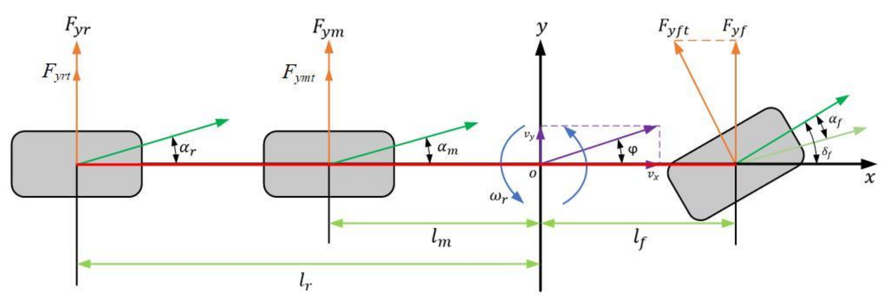
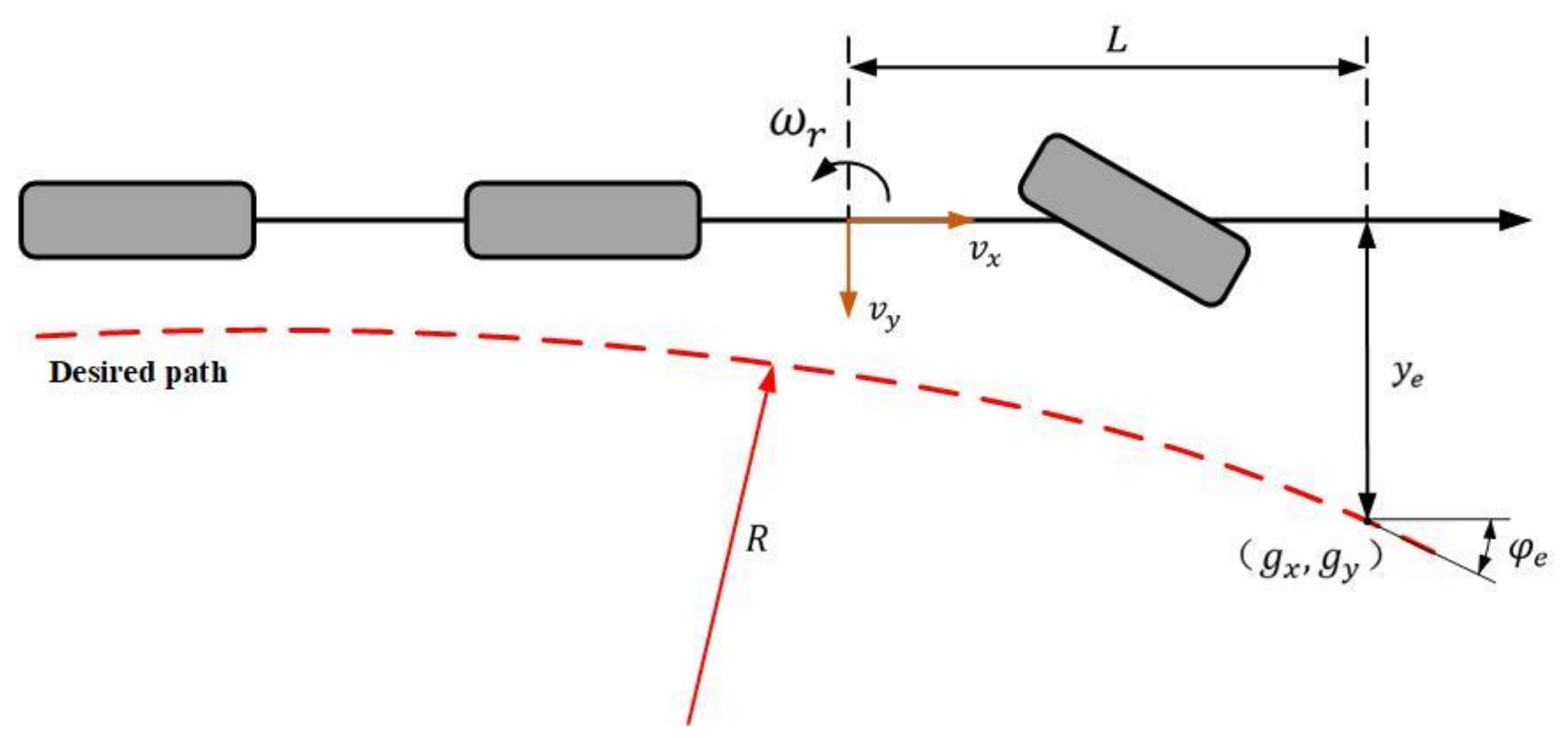
2.1. Tri-Axial Mining Truck Path following the Preview Error Model
2.2. Road Surface Elevation Input Model
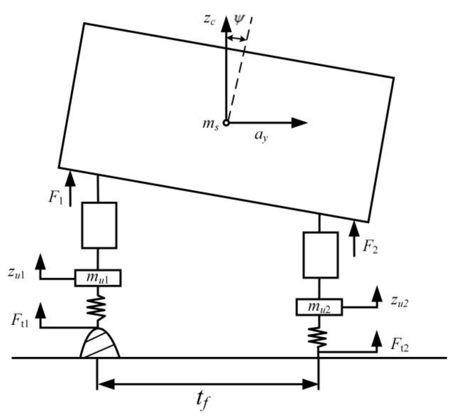
2.3. Calculation of the Trip-Induced Rollover Evaluation Index
3. Path Tracking and Anti-Roll Coordinated Controller Design
3.1. Design of a Steering Anti-Rollover Controller Based on Sliding Mode Control
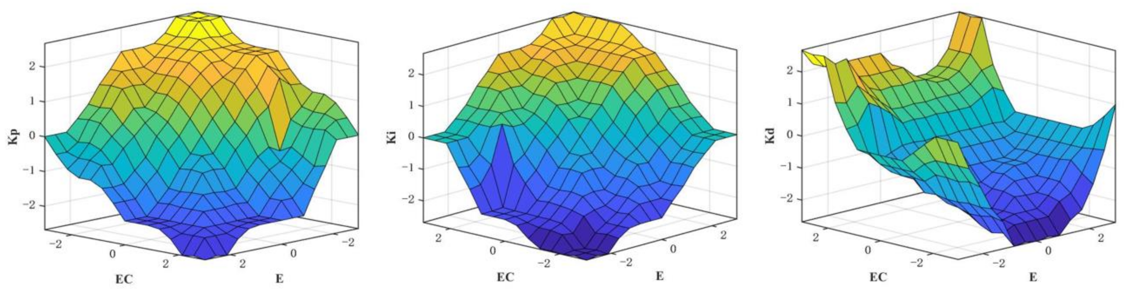
3.2. Design of an Active Suspension Controller Based on Fuzzy PID
3.3. Design of a Path Tracking Controller Based on a Linear Quadratic Regulator (LQR)
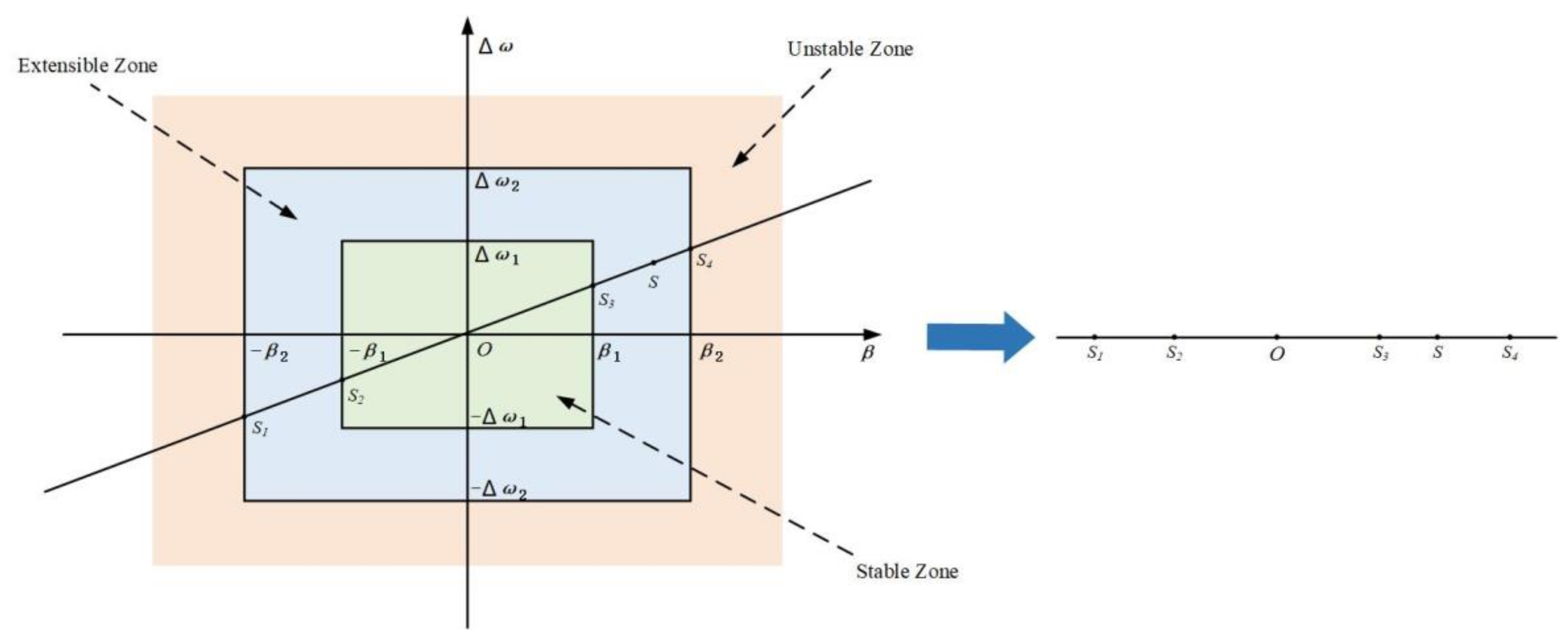
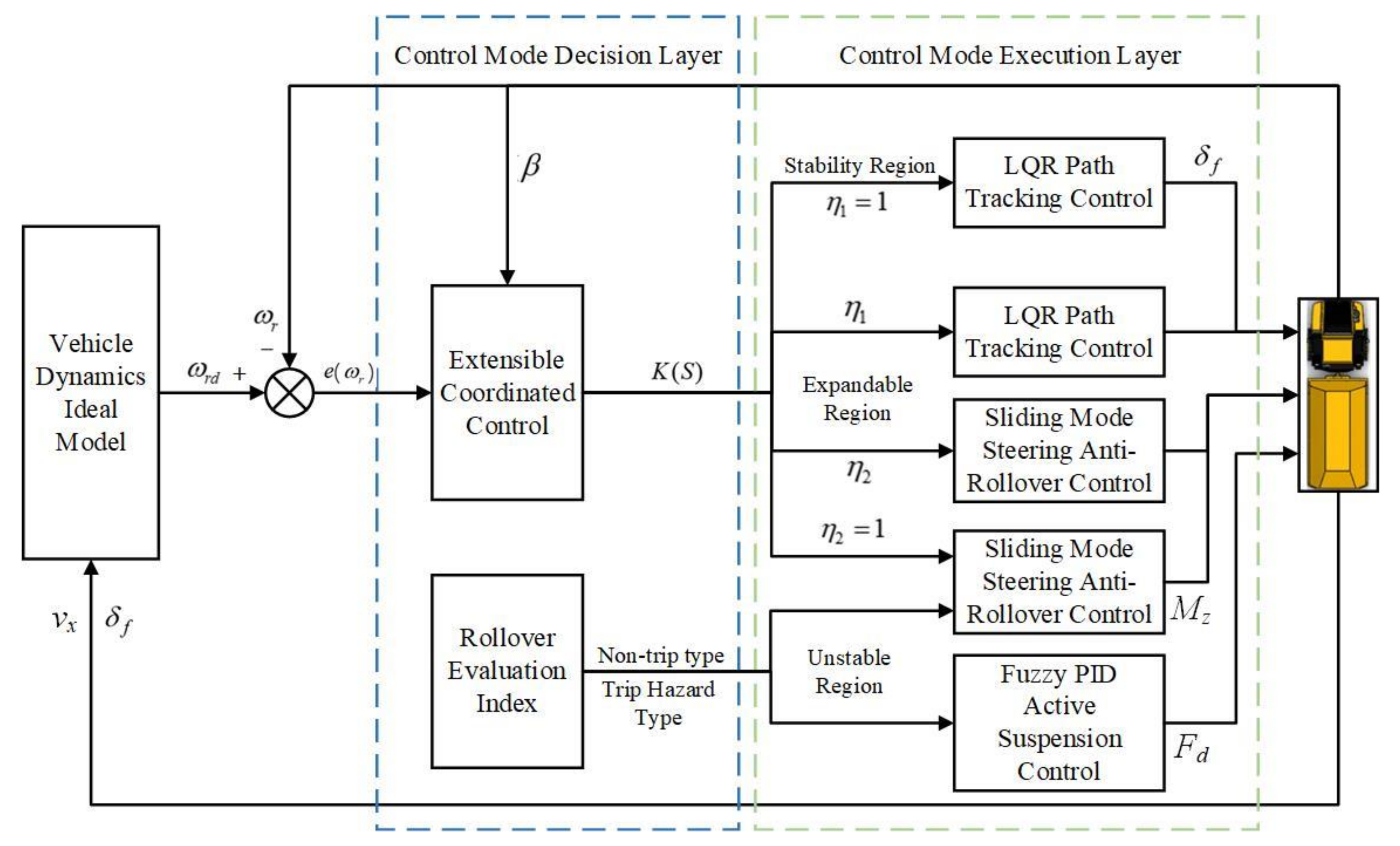
3.4. Design of a Path following and Anti-Roll Coordinated Control System
4. Simulation and Results Analysis
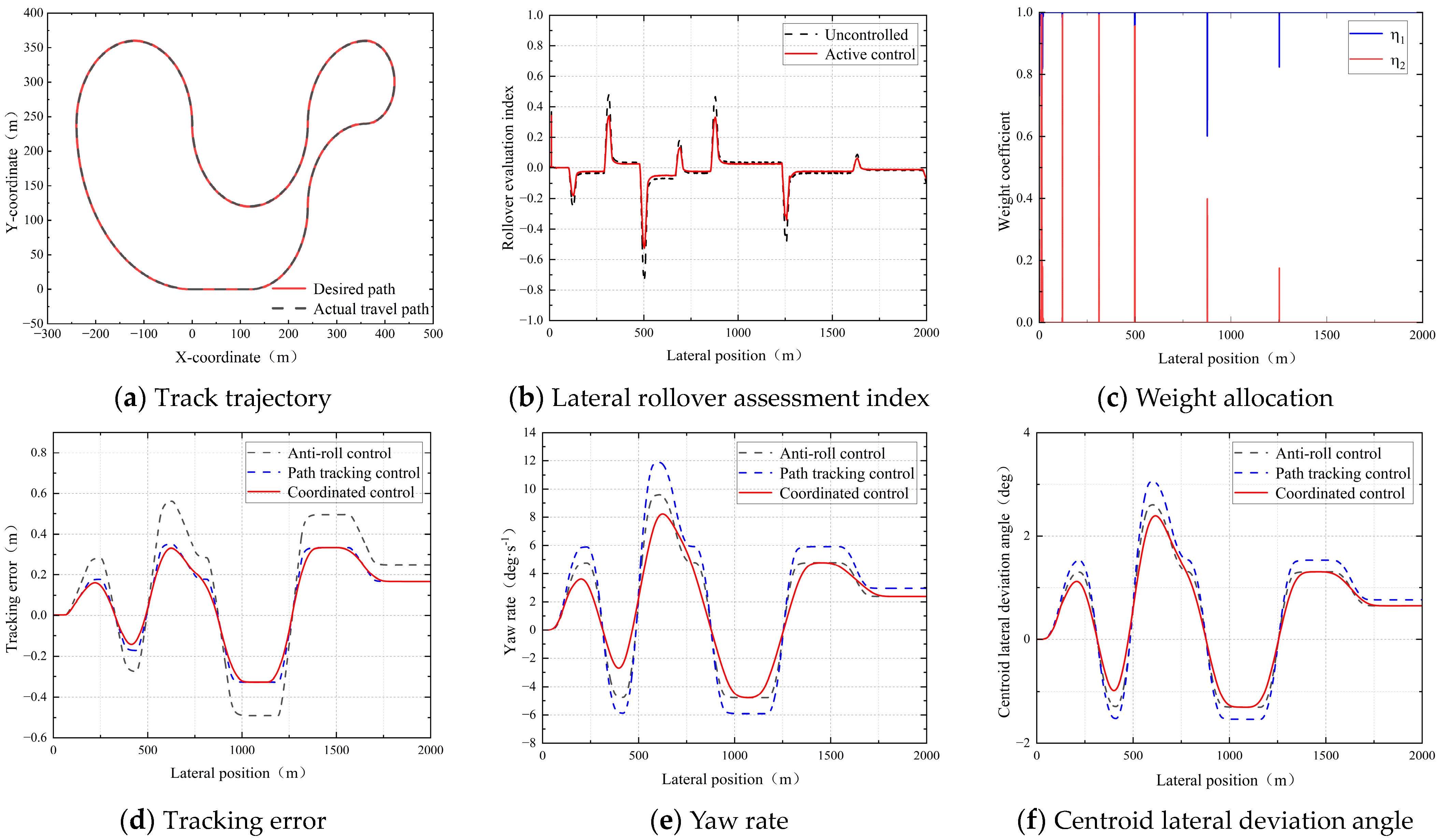
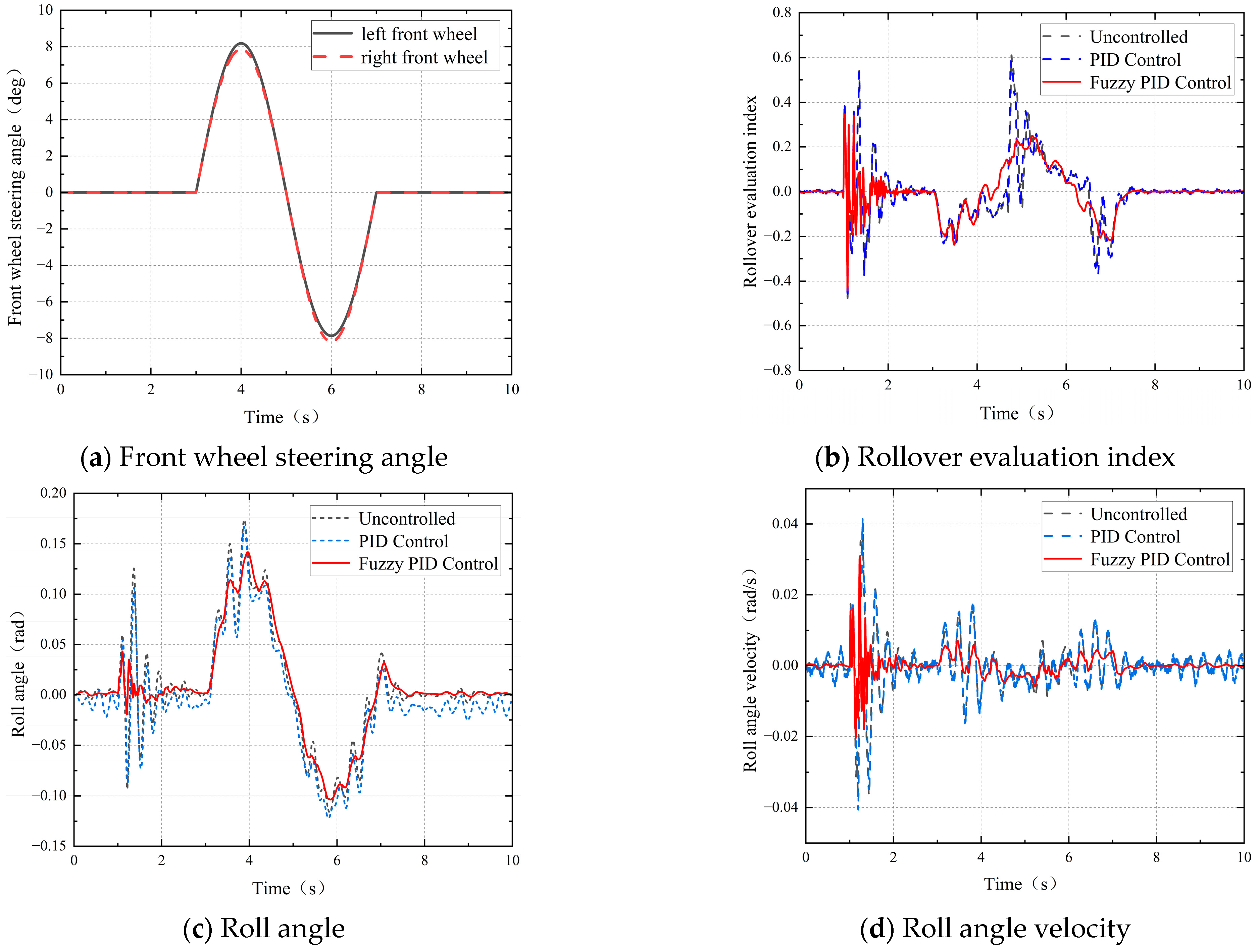
4.1. Simulation Validation under Different Working Conditions
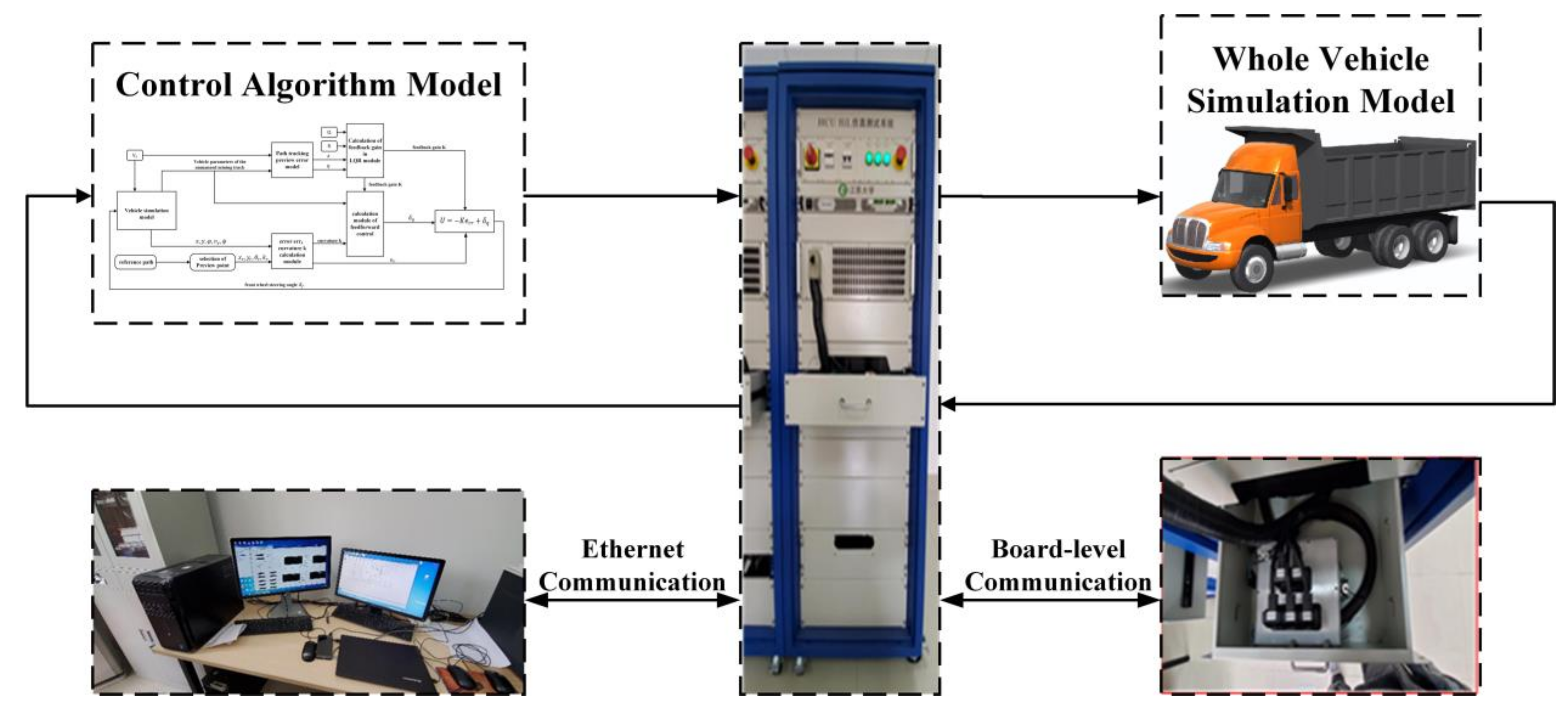
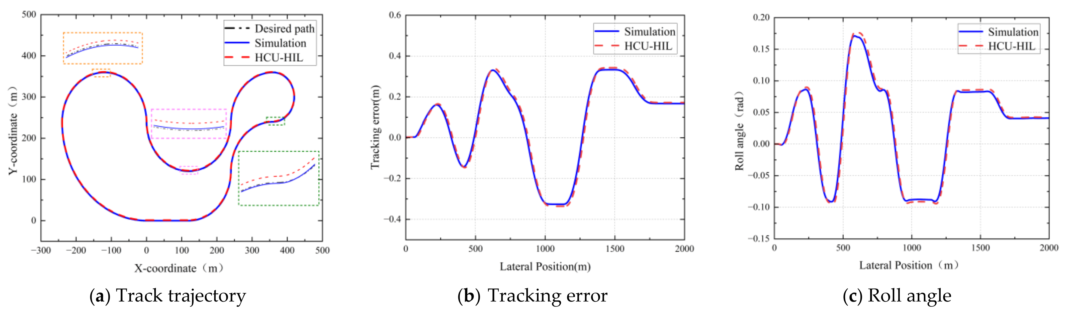
4.2. HCU-HIL Experimental Validation
5. Conclusions
Author Contributions
Funding
Data Availability Statement
Conflicts of Interest
References
- Thompson, R.J.; Rodrigo, P.; Visser, A.T. Mining Haul Roads: Theory and Practice; CRC Press: Boca Raton, FL, USA, 2019. [Google Scholar]
- Akopov, A.S.; Beklaryan, L.A.; Beklaryan, A.L. Cluster-Based Optimization of an Evacuation Process Using a Parallel Bi-Objective Real-Coded Genetic Algorithm. Cybern. Inf. Technol. 2020, 20, 45–63. [Google Scholar] [CrossRef]
- Wang, H.B.; Hu, C.L.; Zhou, J.T.; Feng, L.Z.; Ye, B.; Lu, Y.J. Path tracking control of an autonomous vehicle with model-free adaptive dynamic programming and RBF neural network disturbance compensation. Proc. Inst. Mech. Eng. Part D J. Automob. Eng. 2022, 236, 825–841. [Google Scholar] [CrossRef]
- Jiang, Y.; Xu, X.J.; Zhang, L.; Zou, T.A. Model free predictive path tracking control of variable-configuration unmanned ground vehicle. ISA Trans. 2022, 129, 485–494. [Google Scholar] [CrossRef] [PubMed]
- Wang, Z.J.; Zhou, X.Y.; Wang, J.M. Extremum-Seeking-Based Adaptive Model-Free Control and Its Application to Automated Vehicle Path Tracking. IEEE-ASME Trans. Mechatron. 2022, 27, 3874–3884. [Google Scholar] [CrossRef]
- Lin, F.; Chen, Y.; Zhao, Y.; Wang, S. Path tracking of autonomous vehicle based on adaptive model predictive control. Int. J. Adv. Robot. Syst. 2019, 16, 172988141988008. [Google Scholar] [CrossRef]
- Sánchez, I.; D’Jorge, A.; Raffo, G.; González, A.H.; Ferramosca, A. Nonlinear Model Predictive Path Following Controller with Obstacle Avoidance. J. Intell. Robot. Syst. 2021, 102, 16. [Google Scholar] [CrossRef]
- Song, R.; Ye, Z.; Wang, L.; He, T.; Zhang, L. Autonomous Wheel Loader Trajectory Tracking Control Using LPV-MPC. arXiv 2022, arXiv:2203.08944. [Google Scholar]
- Subari, M.A.; Hudha, K.; Abd Kadir, Z.; Dardin, S.; Amer, N.H. Development of Path Tracking Controller for An Autonomous Tracked Vehicle. In Proceedings of the 2020 16th IEEE International Colloquium on Signal Processing & Its Applications (CSPA 2020), Langkawi, Malaysia, 28–29 February 2020; pp. 126–130. [Google Scholar]
- Mai, T.A.; Dang, T.S.; Duong, D.T.; Le, V.C.; Banerjee, S. A combined backstepping and adaptive fuzzy PID approach for trajectory tracking of autonomous mobile robots. J. Braz. Soc. Mech. Sci. Eng. 2021, 43, 156. [Google Scholar] [CrossRef]
- Wang, R.; Li, Y.; Fan, J.H.; Wang, T.; Chen, X.T. A Novel Pure Pursuit Algorithm for Autonomous Vehicles Based on Salp Swarm Algorithm and Velocity Controller. IEEE Access 2020, 8, 166525–166540. [Google Scholar] [CrossRef]
- Horváth, E.; Hajdu, C.; Korös, P. Novel Pure-Pursuit Trajectory Following Approaches and their Practical Applications. In Proceedings of the 2019 10th IEEE International Conference on Cognitive Infocommunications (COGINFOCOM 2019), Naples, Italy, 23–25 October 2019; pp. 597–601. [Google Scholar]
- Yildiz, H.; Can, N.K.; Ozguney, O.C.; Yagiz, N. Sliding mode control of a line following robot. J. Braz. Soc. Mech. Sci. Eng. 2020, 42, 561. [Google Scholar] [CrossRef]
- Ji, X.; Wei, X.H.; Wang, A.Z.; Cui, B.B.; Song, Q. A novel composite adaptive terminal sliding mode controller for farm vehicles lateral path tracking control. Nonlinear Dyn. 2022, 110, 2415–2428. [Google Scholar] [CrossRef]
- Wang, H.; Liu, B.; Ping, X.; An, Q. Path Tracking Control for Autonomous Vehicles Based on an Improved MPC. IEEE Access 2019, 7, 161064–161073. [Google Scholar] [CrossRef]
- Awad, N.; Lasheen, A.; Elnaggar, M.; Kamel, A. Model predictive control with fuzzy logic switching for path tracking of autonomous vehicles. ISA Trans. 2022, 129, 193–205. [Google Scholar] [CrossRef] [PubMed]
- Xu, S.B.; Peng, H.E. Design, Analysis, and Experiments of Preview Path Tracking Control for Autonomous Vehicles. IEEE Trans. Intell. Transp. Syst. 2020, 21, 48–58. [Google Scholar] [CrossRef]
- Gao, L.; Tang, F.; Guo, P.; He, J. Research on Improved LQR Control for Self-driving Vehicle Lateral Motion. Mech. Sci. Technol. Aerosp. Eng. 2021, 40, 435–441. [Google Scholar]
- Treetipsounthorn, K.; Phanomchoeng, G. Real-Time Rollover Warning in Tripped and Un-tripped Rollovers with A Neural Network. In Proceedings of the International Conference on Control Science and Systems Engineering, Wuhan, China, 21–23 August 2018. [Google Scholar]
- Yim, S. Design of a robust controller for rollover prevention with active suspension and differential braking. J. Mech. Sci. Technol. 2012, 26, 213–222. [Google Scholar] [CrossRef]
- Termous, H.; Shraim, H.; Talj, R.; Francis, C.; Charara, A. Coordinated control strategies for active steering, differential braking and active suspension for vehicle stability, handling and safety improvement. Veh. Syst. Dyn. 2019, 57, 1494–1529. [Google Scholar] [CrossRef]
- Qian, X.G.; Wang, C.Y.; Zhao, W.Z. Rollover prevention and path following control of integrated steering and braking systems. Proc. Inst. Mech. Eng. Part D J. Automob. Eng. 2020, 234, 1644–1659. [Google Scholar] [CrossRef]
- Yang, Z.; Zhao, L.; Zhao, X.; Liu, H. Improvement of Steering Performance for Autonomous Vehicles Based on Preview Model. In Proceedings of the 42nd China Control Conference, Tianjin, China, 24–26 July 2023; p. 6. [Google Scholar]
- Bin, W.; Xuexun, G.; Bo, Y.; Guangpan, L. A Review of the relation Between Road Power Spectral Density and International Roughness Index. Transp. Sci. Technol. 2008, 4, 49–51. [Google Scholar]
- Yonglin, Z.; Jiafan, Z. Numerical simulation of stochastic road process using white noise filtration. Mech. Syst. Signal Process. 2005, 20, 363–372. [Google Scholar] [CrossRef]
- Phanomchoeng, G.; Rajamani, R. New Rollover Index for the Detection of Tripped and Untripped Rollovers. IEEE Trans. Ind. Electron. 2013, 60, 4726–4736. [Google Scholar] [CrossRef]
- Ma, L.; Cheng, C.; Guo, J.F.; Shi, B.H.; Ding, S.H.; Mei, K.Q. Direct yaw-moment control of electric vehicles based on adaptive sliding mode. Math. Biosci. Eng. 2023, 20, 13334–13355. [Google Scholar] [CrossRef] [PubMed]
- Phu, N.D.; Hung, N.N.; Ahmadian, A.; Senu, N. A New Fuzzy PID Control System Based on Fuzzy PID Controller and Fuzzy Control Process. Int. J. Fuzzy Syst. 2020, 22, 2163–2187. [Google Scholar] [CrossRef]
- Kilicarslan, S.; Celik, M. RSigELU: A nonlinear activation function for deep neural networks. Expert Syst. Appl. 2021, 174, 114805. [Google Scholar] [CrossRef]


| e | ||||||||
|---|---|---|---|---|---|---|---|---|
| NB | NM | NS | ZE | PS | PM | PB | ||
| ec | NB | PB | PB | PM | PM | PS | ZE | ZE |
| NM | PB | PB | PM | PS | PS | ZE | NS | |
| NS | PM | PM | PM | PS | ZE | NS | NS | |
| ZE | PM | PM | PS | ZE | NS | NM | NM | |
| PS | PS | PS | ZE | NS | NS | NM | NM | |
| PM | PS | ZE | NS | NM | NM | NM | NB | |
| PB | ZE | ZE | NM | NM | NM | NB | NB | |
| e | ||||||||
|---|---|---|---|---|---|---|---|---|
| NB | NM | NS | ZE | PS | PM | PB | ||
| ec | NB | NB | NB | NM | NM | NS | ZE | ZE |
| NM | NB | NB | NM | NS | NS | ZE | ZE | |
| NS | NB | NM | NS | NS | ZE | PS | PS | |
| ZE | NM | NM | NS | ZE | PS | PM | PM | |
| PS | NM | NS | ZE | PS | PS | PM | PB | |
| PM | ZE | ZE | PS | PS | PM | PM | PB | |
| PB | ZE | ZE | PS | PM | PM | PB | PB | |
| e | ||||||||
|---|---|---|---|---|---|---|---|---|
| NB | NM | NS | ZE | PS | PM | PB | ||
| ec | NB | PS | NS | NB | NB | NB | NM | PS |
| NM | PS | NS | NB | NM | NM | NS | ZE | |
| NS | ZE | NS | NM | NM | NS | NS | ZE | |
| ZE | ZE | NS | NS | NS | NS | NS | ZE | |
| PS | ZE | ZE | ZE | ZE | ZE | ZE | ZE | |
| PM | PB | PB | PS | PS | PS | PS | PB | |
| PB | PB | PM | PM | PM | PS | PS | PB | |
| Parameter | Name | Numerical Value (Unit) |
|---|---|---|
| m | Vehicle mass | 8525 kg |
| lf | Distance from the front axle to the center of gravity | 1.3 m |
| lm | Distance from the mid-axle to the center of gravity | 4.5 m |
| lr | Distance from the rear axle to the center of gravity | 5.7 m |
| h | Center of gravity height | 1.02 m |
| Cij | Tire stiffness | −301,385 N/rad |
| IZ | Rotational inertia | 35,000 kg·m2 |
| Uncontrolled | PID Control | Fuzzy PID Control | Maximum Degree of Optimization (+) | |||||
|---|---|---|---|---|---|---|---|---|
| Vehicle rollover condition | Trip | Non-trip | Trip | Non-trip | Trip | Non-trip | Trip | Non-trip |
| Rollover evaluation index | 0.56 | 0.6 | 0.5 | 0.54 | 0.38 | 0.23 | 32.1% | 62.7% |
| Roll angle(max)/rad | 0.125 | 0.174 | 0.11 | 0.162 | 0.048 | 0.145 | 61.6% | 16.7% |
| Roll angle velocity (max)/rad·s−1 | 0.041 | 0.018 | 0.035 | 0.016 | 0.03 | 0.007 | 26.8% | 61.1% |
| Anti-Roll Control | Path Tracking Control | Coordinated Control | Maximum Degree of Optimization (+) | |
|---|---|---|---|---|
| Tracking error(max)/m | 0.59 | 0.35 | 0.32 | 45.7% |
| Yaw rate(max)/deg·s−1 | 9.8 | 12 | 8.1 | 32.5% |
| Centroid lateral deviation angle(max)/deg | 2.6 | 3 | 2.4 | 20.0% |
Disclaimer/Publisher’s Note: The statements, opinions and data contained in all publications are solely those of the individual author(s) and contributor(s) and not of MDPI and/or the editor(s). MDPI and/or the editor(s) disclaim responsibility for any injury to people or property resulting from any ideas, methods, instructions or products referred to in the content. |
© 2024 by the authors. Licensee MDPI, Basel, Switzerland. This article is an open access article distributed under the terms and conditions of the Creative Commons Attribution (CC BY) license (https://creativecommons.org/licenses/by/4.0/).
Share and Cite
Wang, R.; Wan, J.; Ye, Q.; Ding, R. Path Tracking and Anti-Roll Control of Unmanned Mining Trucks on Mine Site Roads. World Electr. Veh. J. 2024, 15, 167. https://doi.org/10.3390/wevj15040167
Wang R, Wan J, Ye Q, Ding R. Path Tracking and Anti-Roll Control of Unmanned Mining Trucks on Mine Site Roads. World Electric Vehicle Journal. 2024; 15(4):167. https://doi.org/10.3390/wevj15040167
Chicago/Turabian StyleWang, Ruochen, Jianan Wan, Qing Ye, and Renkai Ding. 2024. "Path Tracking and Anti-Roll Control of Unmanned Mining Trucks on Mine Site Roads" World Electric Vehicle Journal 15, no. 4: 167. https://doi.org/10.3390/wevj15040167
APA StyleWang, R., Wan, J., Ye, Q., & Ding, R. (2024). Path Tracking and Anti-Roll Control of Unmanned Mining Trucks on Mine Site Roads. World Electric Vehicle Journal, 15(4), 167. https://doi.org/10.3390/wevj15040167