A Review of Lithium-Ion Battery State of Charge Estimation Methods Based on Machine Learning

Abstract

With the advancement of machine-learning and deep-learning technologies, the estimation of the state of charge (SOC) of lithium-ion batteries is gradually shifting from traditional methodologies to a new generation of digital and AI-driven data-centric approaches. This paper provides a comprehensive review of the three main steps involved in various machine-learning-based SOC estimation methods. It delves into the aspects of data collection and preparation, model selection and training, as well as model evaluation and optimization, offering a thorough analysis, synthesis, and summary. The aim is to lower the research barrier for professionals in the field and contribute to the advancement of intelligent SOC estimation in the battery domain.

1. Introduction

Lithium-ion batteries are high-energy-density and long-life energy storage devices widely used in electric vehicles, renewable energy, and other fields. Estimating the state of charge (SOC) of lithium batteries plays a significant role in battery management. Accurate SOC estimation can enhance the performance, lifespan, and safety of the battery [1]. However, lithium batteries, characterized by their nonlinear and time-varying electrochemical properties, pose considerable challenges in terms of the observation of their internal states through external instruments. Therefore, the SOC can only be estimated through a series of parameters or external characteristics. Currently, the SOC estimation methods for lithium batteries are primarily categorized into direct and indirect methods, as illustrated in Figure 1. Traditional SOC estimation methods include the ampere-hour integration method [2], open-circuit voltage method [3], equivalent circuit model method [4], adaptive filtering methods (including Kalman filtering [5] and extended Kalman filtering [6,7,8]), and nonlinear observer methods (including the sliding mode observer [9,10], proportional-integral observer [11], and nonlinear observer [12]). The advantages and disadvantages of the traditional approach are summarized in

Table 1. Advantages and disadvantages of traditional methods.

	Method	Advantage	Disadvantage
Direct method	Ampere-Hour Integration	Simple and convenient Low computational complexity	Depends on initial SOC value Accumulative error Overlooks capacity decay Needs precise equipment
	Open Circuit Voltage	Simple and easy to use	Long measurement downtime Dynamic condition limitations
Model method	Electrochemical Model	Reflects the internal characteristics of the battery	Complex model and parameter setup High computational complexity
	Equivalent Circuit Model	Easy to understand Fewer parameters	Complex model and parameter setup High computational complexity
	Kalman Filter (KF)	Simple and efficient Real-time estimation.	Linear model constraints Noise restrictions
	Extended Kalman Filter (EKF)	Deals with low nonlinear systems Real-time estimation	Nonlinear system underperforms Jacobian matrix calculation Surpasses KF in complexity Complex parameter tuning
	Unscented Kalman Filter (UKF)	Highly nonlinear capability More accurate than EKF No Jacobian matrix calculation	Exceeds the KF/EKF in complexity Depends on the choice of parameters (e.g., sigma points and weights)
	Particle Pilter (PF)	Handles highly nonlinear and non-Gaussian systems Handles multi-modal distribution	High computational complexity Poor real-time estimation Needs a large number of samples
Nonlinear observer	Sliding Mode Observer	Good robustness Quick response	Chattering phenomenon Depends on the accuracy of the system model

.

The traditional methods for estimating the SOC of lithium-ion batteries are confronted with challenges such as complex battery models, sensitivity to model parameters, poor adaptability, and high computational complexity [13]. The effectiveness of these methods is constrained by the uncertainties and complexities inherent in battery models, highlighting the necessity for advancements in the real-time capabilities, accuracy, robustness, and adaptability of SOC estimations. In contrast, data-driven approaches to SOC estimation capitalize on big data and machine-learning technologies, which do not require the construction of precise battery models. These approaches primarily depend on the quality of the collected datasets, as well as the selection and optimization of the model, employing extensive data to train models that discern the nonlinear mapping relationships between the input features and SOC, thus enabling more accurate SOC estimations. Machine-learning models possess formidable nonlinear mapping capacities, robust generalization, and adaptability [14]. Consequently, data-driven SOC estimation methods for lithium batteries have rapidly developed.

Furthermore, since the estimation issues concerning the SOC and SOH can be defined as the estimation of nonlinear states and parameters, respectively, and considering that state estimation and parameter estimation are closely related, they can be addressed using similar methodologies [15,16]. Therefore, this paper primarily focuses on a comprehensive review of SOC estimation.

This paper’s contributions are primarily as follows:

• The limitations of traditional SOC estimation methods are summarized. The advantages and necessity of machine-learning SOC estimation are presented.
• The datasets commonly used by researchers and the processing methods for the datasets are summarized and sorted out.
• The models of SOC estimation using traditional neural networks and deep neural networks are introduced, and the advantages and disadvantages of various models are compared.
• The impact of model hyperparameter settings and tuning methods on model performance is discussed. Factors affecting model performance are explored, and reference methods for model validation are established.
• The research needs, challenges faced, and areas requiring improvement for machine-learning-based SOC estimation are clarified.

The subsequent sections of this paper are organized as follows. The Section 2 outlines the steps for SOC estimation based on machine learning. The Section 3 discusses the datasets and data-processing methods. The Section 4 examines machine-learning algorithms for SOC estimation. The Section 5 addresses the SOC evaluation criteria and methods for setting and tuning hyperparameters. The Section 6 explores the challenges faced and directions for improvement. The Section 7 provides a comprehensive summary of the entire paper.

2. Methods

The methodology for SOC estimation utilizing machine learning encompasses three primary phases: data collection and preparation, model selection and training, and model evaluation and tuning.

Data collection and preparation involve transforming the gathered raw battery data into feature vectors suitable for machine-learning algorithms. This process includes data cleaning, preprocessing, and feature engineering of the relevant datasets. Model selection and training involve choosing the appropriate machine-learning algorithms and models based on specific requirements, including dividing the data into training, testing, and validation sets. Model evaluation and tuning refer to assessing and improving the model based on certain evaluation metrics or systems, involving adjustments to the hyperparameters, feature selection, and model structure. The specific steps involved in SOC estimation are illustrated in Figure 2.

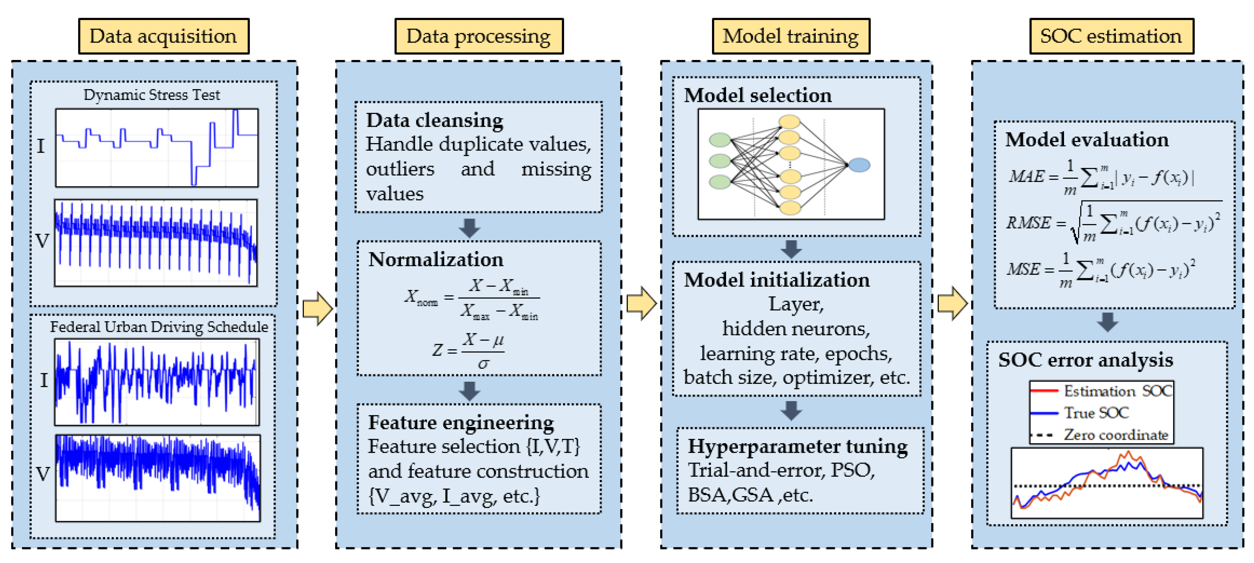
3. Data Collection and Preparation

3.1. Data Collection

In machine-learning-based SOC estimation, the input of a substantial volume of data into the model for training is essential. The foundation for successful model training lies in the availability of high-quality and authoritative datasets. The closer the training data is to the actual battery operating conditions, the more precise the algorithm model’s output, underscoring the undeniable importance of the dataset.

In the papers reviewed, the datasets utilized primarily originate from three sources. The first category includes datasets obtained from different types of battery discharge experiments conducted under laboratory conditions using battery testing platforms, such as Constant Current–Constant Voltage (CC–CV) tests or constant current pulse test datasets. The second category comprises datasets publicly released by authoritative institutions or research institutes, which also include real-world data from electric vehicle operations, such as the CALCE dataset from the University of Maryland’s Battery Laboratory and the RBUDS from NASA. The third category is datasets derived from simulation software, like the ADVISOR2002 dataset for advanced vehicle simulation. These datasets can be primarily classified into two categories: battery discharge characteristics and vehicle driving characteristics. Analyzing these two types of features reveals that the battery discharge properties are the predominant factor. Most researchers use the current voltage, current, and temperature as the main input features, while a few use the averages, driving data, polarization states, or other data as supplementary inputs.

Table 2. Common datasets.

	Data Source	Data Content	Data Characteristics
1	Dataset of new energy vehicle data platform [17].	Includes the total voltage, monomer current, cell voltage, temperature, etc., and the error identification code.	Encompasses core vehicle system parameters and BeiDou navigation position data.
2	ADVISOR2002 dataset of advanced vehicle simulation software [18].	Simulation software provides the voltage, current, temperature, and SOC values.	Simulation mimics comprehensive electric vehicle battery data under varied conditions.
3	NASA dataset [19].	Features charge/discharge data across conditions, temperature states, and aging, with randomness and uncertainty.	Battery cycles through random current conditions.
4	University of Maryland Battery Laboratory (CACLE) [20].	Discharge data under three different discharge conditions, including voltage, current, temperature and other parameters.	Discharge conditions include DST, US06, and FUDS.
5	Panasonic 18650PF lithium-ion battery dataset of McMaster University, Canada [21].	Includes time information, discharge capacity, power, battery voltage, current, energy, battery shell temperature, incubator temperature, etc.	Covers temperatures of 0 °C, 10 °C, and 25 °C.

provides a summary of the commonly used dataset sources and their characteristics.

High-quality datasets can enhance the accuracy of SOC estimation, strengthen the robustness and generalizability of the model, and improve the model’s overall performance. In addition to the aforementioned datasets, some researchers have also utilized the following datasets: Stanford Cycle Life Prediction Dataset [22], Stanford Fast-Charging Optimization Dataset [23], Oxford Battery Degradation Dataset [24], Sandia National Laboratories [25], Poznan University of Technology Laboratories [26], and Panasonic 18650PF Li-Ion Battery Dataset of the University of Wisconsin-Madison [27].

These datasets contribute significantly to the field by providing diverse and comprehensive data, enabling more accurate predictions and optimizations regarding SOC estimation models.

3.2. Data Preparation

The goal of data cleaning and preprocessing is to enhance the quality and usability of the data, laying a solid foundation for subsequent feature engineering and modeling. Data cleaning involves identifying and rectifying errors or inconsistencies in the data, such as missing values, outliers, or incorrect entries. Preprocessing, on the other hand, involves transforming the raw data into a format more suitable for analysis, which may include normalization, scaling, encoding categorical variables, and handling missing data. Feature engineering aims to extract effective features from the raw data that can reflect the state and performance of the battery for use in model training and prediction. This process includes selecting relevant features, creating new features through domain knowledge, and transforming features to improve their relationship with the target variable.

Table 3. Common methods of data preparation.

Method	Main Operation
Data cleaning [17]	Remove duplicate values, handle abnormal values and fill in missing values.
Statistical characteristics [17]	Calculate statistical measures like the mean, variance, max, min, and median to characterize battery data distribution and variation.
Data normalization [28,29,30]	Normalize features across dimensions using min–max and standardization.
Data conversion [29]	Apply logarithmic and exponential transformations for nonlinear data to linearize and enhance model fit.
Data dimensionality reduction [31]	Use PCA and other techniques for dimensionality reduction, converting high-dimensional data into a compact feature space.
Data balance [32]	Employ under-sampling and over-sampling to balance the dataset and improve the minority class recognition.
Time characteristics [32]	Extract time features from timestamps to identify periodicity and trends.
Data smoothing [32]	Smooth data to lessen noise and sharp fluctuations.
Differential feature [32]	Perform differential analysis of battery data, using the differences between consecutive time points as features.

summarizes the common methods and operations used in data preparation, providing a comprehensive overview of the techniques employed to ensure the data are optimized for machine-learning applications in SOC estimation.

Gan et al. [17] utilized SQL queries to perform data cleaning and preprocessing from a MySQL database, selecting a dataset that represents the range of most frequent charge–discharge cycles in daily vehicle use (SOC between 90% and 20%) for the SOC estimation training. Liu et al. [28], in their study utilizing a convolutional neural network (CNN) model, incorporated a batch normalization layer between each convolutional layer and its corresponding activation function. This addition aimed to ensure a more uniform distribution across the network’s layers. Altman et al. [29], aiming to eliminate the differences in the numerical ranges of different features, adopted feature-scaling methods such as normalization, standardization, and centering to process data. Gan et al. [17] conducted a correlation analysis between the feature fields and SOC using the Spearman correlation coefficient. They found a correlation between the total voltage, maximum and minimum cell voltage, highest and lowest temperature, and the label field SOC, while the speed and total current showed a low correlation with the SOC. Furthermore, they constructed five new feature groups based on artificial prior knowledge and added them to the original pure electric vehicle operational data, thereby expanding the data dimensionality. Li [31] employed Principal Components Analysis (PCA) to extract the most relevant input features from a multitude of data, including the integral and differential of the voltage and current. These features were then input into a BP neural network, effectively reducing the dimensionality of the inputs while retaining a wide range of input information, which led to improvements in the computational complexity and estimation accuracy.

Although data processing involves numerous operations, most researchers favor simpler procedures. In terms of preprocessing, the wide range of data presents a challenge: battery voltage values span from 2.5 to 4.2, current values range from −4 to 2, SOC values lie between 0 and 1, and temperature values vary from 0 to 45 °C. These significant differences in the data ranges can cause the model to prioritize certain features over others during the parameter optimization process. Therefore, normalization and standardization are generally necessary. In terms of feature engineering, most features need to be manually extracted or extracted with the aid of software from the dataset. Most researchers use simple sampling values such as the voltage, current, temperature, average voltage, and average current as inputs. A minority of researchers use the means, derivatives, integrals, and other more complex features extracted as inputs.

4. Model Selection and Training

Machine-learning models exhibit a potent capacity for nonlinear mapping, a characteristic that confers significant advantages, notably their robust generalization capabilities. However, a notable drawback of these methods is their reliance on extensive sample training, coupled with the high computational demand. This includes both the cost of high-performance processing chips and the time required for training samples. The selection of a model should be a comprehensive process, taking into account factors such as the fitting accuracy, cost, robustness, and complexity [33,34,35].

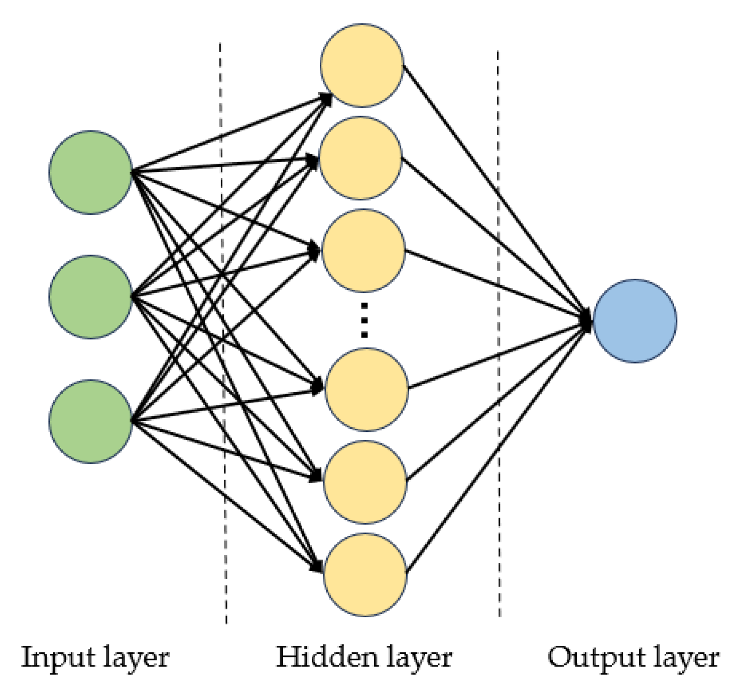
4.1. Artificial Neural Networks

Artificial Neural Networks (ANNs) [36] can be broadly categorized into traditional neural networks and deep-learning networks. Traditional neural networks are composed of just an input layer, a single hidden layer, and an output layer. An ANN structure diagram is shown in Figure 3. Typical examples of traditional neural networks include the Back Propagation Neural Network (BPNN) [37], Wavelet Neural Network (WNN) [38], Radial Basis Function Neural Network (RBFNN) [39], and Extreme Learning Machine (ELM) [40], among others.

4.1.1. BPNN Network

The feedforward Back Propagation Neural Network (BPNN) [41] represents the quintessential model of neural networks, employing nonlinear monotonic univariate functions as activation functions. The training process for the BPNN is centered on identifying the optimal values for weights and biases to minimize the loss function. With the maturity of BPNN technology, numerous hybrid algorithms have emerged, integrating with the BPNN.

Yin et al. [42] enhanced the BPNN using the Levenberg–Marquardt (L–M) algorithm, a numerical optimization technique, effectively boosting the network’s convergence speed. Their findings demonstrated that the error between the actual and predicted SOC values remained within a 6% range, validating the feasibility of the improved BPNN for estimating the SOC. However, the model’s tendency to become trapped in local minima remained unresolved.

To address this, Yu et al. [43] combined the Genetic Algorithm (GA) with the BPNN. The improved GA-BP network not only maintained excellent nonlinear mapping and data prediction capabilities but also ameliorated the BPNN’s susceptibility to local minima. This refinement reduced the error margin between the actual and predicted SOC values to between 2% and 3%, enhancing the SOC estimation accuracy. Furthering these advancements, Xu et al. [44] proposed the integration of the Whale Optimization Algorithm (WOA) with the BPNN. The WOA-BP neural network algorithm overcame the issues of slow convergence and local minima that are inherent in the traditional BPNN. Comparative analysis against the GA-BP algorithm, using metrics such as the MAE, MSE, and RMSE, revealed that the WOA-BP neural network algorithm exhibits superior robustness and precision.

4.1.2. RBFNN Network

The Radial Basis Function Neural Network (RBFNN) [45] employs radial basis functions as activation functions. The RBFNN offers advantages such as local approximation, excellent interpolation capabilities, and reduced computational complexity, aligning with real-time design requirements. The standard RBFNN typically estimates with a maximum error of approximately 5%. To optimize the RBFNN model, many researchers have made enhancements and improvements.

Zhang et al. [45] combined the Particle Swarm Optimization (PSO) algorithm with RBF networks, resulting in the PSO-RBFNN, which achieved SOC prediction errors of within 2.5%. Although the improved RBFNN method requires more training time compared to the traditional approach, its root mean square error is only half that of the traditional method. However, the PSO has the potential to lead the PSO-RBFNN model into local minima, causing an increase in the estimation error variability.

Li et al. [46] utilized the Backtracking Spiral Algorithm (BSA) to optimize the RBF network, reducing the maximum estimation error of the BSA-RBFNN to within 2%, further enhancing the SOC estimation accuracy. To determine the optimal number of neurons in the hidden layer for modeling nonlinear relationships, Chang [47] employed the Orthogonal Least Squares Algorithm (OLSA). Additionally, an Adaptive Genetic Algorithm (AGA) was used to train the centers, widths, and weights of the RBFNN as an alternative to traditional stochastic gradient descent. Comparative results with the BPNN across various discharge experiments showed that the RBFNN model exhibits superior performance.

4.1.3. ELM and WNN Networks

In the context of neural networks, Extreme Learning Machines (ELMs) utilize activation functions for hidden layer neurons that can be any function with a range between (0, 1). Unlike the BPNN and RBFNN, an ELM does not employ backpropagation algorithms for weight and bias updates. Instead, it sets these parameters using the Moore–Penrose generalized inverse matrix. On the other hand, Wavelet Neural Networks (WNNs) use wavelet functions as activation functions for the hidden layer [44]. Compared to the BPNN, RBFNN, and ELM, the WNN combines the wavelet decomposition properties with the nonlinear approximation capabilities of neural networks, avoiding local optima issues and enhancing the convergence speed.

Cui et al. [48] conducted research on hybrid adaptive wavelet neural networks and multi-layer adaptive WNNs. They optimized the employed wavelet neural network estimation models using particle swarm optimization and the L–M. Extensive experimental analysis validated the effectiveness of the SOC estimation algorithms based on the studied wavelet neural network models.

Xie et al. [49] proposed an improved WNN model that optimized the weights and thresholds of the WNN model using a GA. The results showed that the GA-WNN provided more accurate SOC estimation and exhibited better convergence properties.

To accelerate the wavelet network parameter optimization and enhance the SOC estimation accuracy, Sun [38] introduced an algorithm based on the Hausdorff derivative for WNN parameter optimization. This method improved the parameter optimization for wavelet neural networks and demonstrated its effectiveness through verification experiments.

Song et al. [50] presented a battery SOC estimation model based on an ELM. The model utilized voltage and current data obtained from discharge experiments under different currents for training and prediction. A comparison of the prediction performance with the BPNN revealed that the ELM had higher estimation accuracy and a significantly faster network training speed. The ELM’s performance was significantly influenced by the training time and the number of neurons in the hidden layer. To address this issue, Anandhakumar [51] and colleagues used an improved optimization algorithm called the Honey Badger Optimization Algorithm (HBA) to select appropriate hidden neurons, resulting in enhanced SOC estimation accuracy. The model achieved an accuracy of 97% in the FUDS drive cycle and 99% in the US06 drive cycle, making it suitable for real-time online estimation.

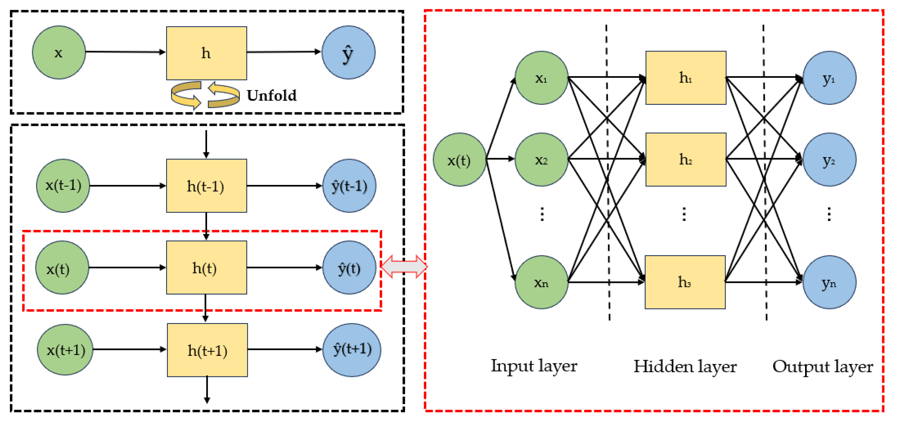
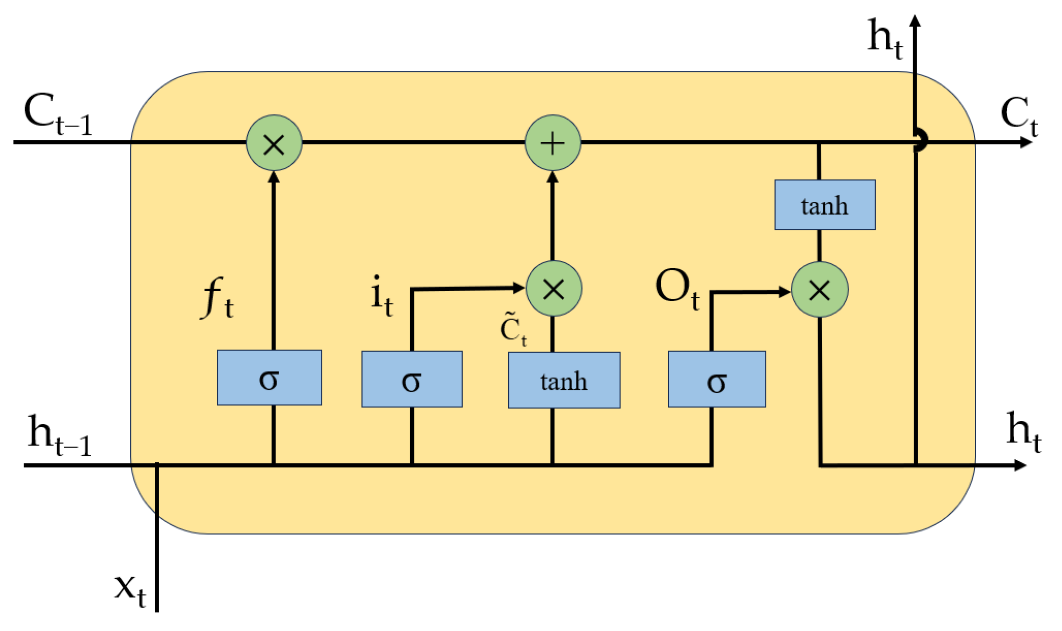
4.2. Deep Neural Network

The ongoing advancement of deep-learning algorithms has led many researchers to focus on deeper neural networks. Traditional feedforward neural networks often only fit the nonlinear mapping relationship between the input and output based on the current moment’s input features. In contrast, deep neural networks, a subset of deep-learning algorithms, utilize multiple hidden layers and are capable of mapping complex and nonlinear functions. They typically exhibit higher accuracy compared to traditional neural networks [52,53].

Common deep-learning models include Convolutional Neural Networks (CNNs) [54] and Recurrent Neural Networks (RNNs) [55]. CNNs are well-suited for tasks involving grid-like data such as images, as they can automatically learn hierarchical features. On the other hand, RNNs are particularly useful for sequences of data, as they can capture temporal dependencies and context information. The use of deep neural networks, like CNNs and RNNs, has significantly contributed to the success of various machine-learning and artificial intelligence applications.

The typical architecture of a CNN consists of multiple layers, including convolutional layers, pooling layers, fully connected layers, and an output layer [56]. The structure of a CNN is shown in Figure 4. The presence of convolutional processes in the CNN allows for faster learning and reduces the memory requirements. This design is particularly effective for tasks involving grid-like data, such as images. On the other hand, RNNs have a short-term “memory” property, where the information in each hidden layer at a given time step depends on the input at that time step and the hidden layer from the previous time step [57]. A structure diagram of the RNN is shown in Figure 5. The corresponding formulas are (1) and (2).

$$h(t)=f(W_{hh}h(t-1)+W_{ih}x(t)+b_h)$$

(1)

$$\stackrel{\wedge }{y}(t)=g(W_{ho}h(t)+b_y)$$

(2)

$x(t)$ is the input at the current time step, $t$. $h(t)$ is the hidden state at the current time step, $t$. $h(t-1)$ is the hidden state from the previous time step, $t-1$. $W_{ih}$, $W_{hh}$, $W_{ho}$ is the connection weight matrix. $y_t$ is the output generated by the output layer at the current time step. $b_h$ and $b_y$ are the bias terms. $f$ and $g$ are the activation functions. In simple terms, the updating of the hidden state in an RNN network is determined by the input at the current time step, $x(t)$, and the hidden state from the previous time step, $h(t-1)$.

However, RNNs suffer from the vanishing gradient or exploding gradient problem when dealing with sequences of data over multiple time steps, limiting their performance. To address this issue, researchers have developed several variants of RNNs. The three mainstream variants of RNNs are Long Short-Term Memory (LSTM) [58], Bi-directional Long Short-Term Memory (Bi-LSTM) [59], and Gated Recurrent Unit (GRU) [60]. LSTM introduces forget gates, input gates, and output gates to mitigate the gradient vanishing problem that exists in traditional RNNs. The structure of the LSTM is shown in Figure 6. The corresponding formula is given in (3)–(8). While this improves the gradient flow, LSTM has a more complex internal structure and increased computational complexity compared to traditional RNNs. The GRU is a modification of LSTM that simplifies the architecture. In contrast to LSTM, which has separate gates for forgetting and updating states, the GRU uses a single gate unit to control both the forgetting and updating processes. This results in a simpler parameter structure and reduced computational complexity compared to LSTM. Both the LSTM and GRU variants have been widely adopted in sequence-modeling tasks, offering solutions to the vanishing gradient problem and improving the performance of RNNs [61].

$$f_t=\sigma (W_f\cdot [h_{t-1},x_t]+b_f)$$

(3)

$$i_t=\sigma (W_i\cdot [h_{t-1},x_t]+b_i)$$

(4)

$${\tilde{C}}_t=\tanh (W_C\cdot [h_{t-1},x_t]+b_{\mathrm{c}})$$

(5)

$$C_t=f_t\ast C_{t-1}+i_t\ast {\tilde{C}}_t$$

(6)

$$o_t=\sigma (W_o\cdot [h_{t-1},x_t]+b_o)$$

(7)

$$h_t=o_t\ast \tanh (C_t)$$

(8)

$f_t$, $i_t$ and $o_t$ are the activation values of the different gates. $\sigma$ is the sigmoid function.$W_f$, $W_i$, $W_C$ and $W_o$ comprise the weight matrix. $b_f$, $b_i$, $b_{\mathrm{c}}$ and $b_o$ are the bias terms, and $[h_{t-1},x_t]$ represents the concatenation of $h_{t-1}$ and $x_t$. $C_t$ is the cell state, while $C_{t-1}$ is the cell state from the previous time step. ${\tilde{C}}_t$ is a tanh layer that creates a new candidate value vector.

Hannan et al. [62] introduced a Fully Convolutional Network (FCN) composed of four temporal convolutions for estimating the SOC. The FCN differs from CNNs in that it transforms the fully connected layers typically found at the end of a CNN into convolutional layers. It employs global average pooling to prevent overfitting. The results showed that this model achieved an RMSE of 0.85% and an MAE of 0.7% at room temperature. The FCN’s unique approach combines the automatic feature extraction capabilities of CNNs with the time-series prediction abilities of RNNs.

Zhang et al. [63] combined a CNN and LSTM to create a CNN-LSTM model with the introduction of an attention mechanism. They utilized one-dimensional convolution to capture the spatial features within measurement variables and employed LSTM to capture the features between the current output and past inputs. The attention mechanism allowed the model to focus on key parts of the input data, thereby improving the overall performance and accuracy. The average prediction error at different temperatures reached 0.89%. This model aims to balance the consideration of temporal aspects while enhancing the estimation accuracy.

To augment the robustness and adaptability of their model, Liu et al. [28] introduced a CNN-GRU hybrid, ingeniously integrating the CNN with the GRU. It demonstrated good performance in unknown operating conditions. In cases where the initial SOC value is unknown, the CNN-GRU neural network rapidly converges to the reference values. This network does not require weight adjustments based on the test conditions, complex feature extraction such as averaging or integration, and does not rely on battery models, filtering, or algorithms. This approach streamlines SOC estimation while maintaining accuracy and adaptability.

Because the estimation of the SOC of lithium batteries can be viewed as a time-series problem, it is related not only to the current moment’s input features but also to previous time steps’ input features. This makes RNNs particularly suitable for SOC estimation. However, using a standalone RNN network for SOC estimation can lead to the vanishing gradient or exploding gradient problem over multiple time steps. Therefore, researchers have mostly focused on studying variants of RNNs or algorithmic models that combine RNNs.

Ma et al. [64] trained and validated an LSTM model to estimate the SOC using a publicly available dataset provided by Phillip Kollmeyer. The estimation error RMSE ranged from 1% to 1.8%. Li et al. [65] were the first to propose using a GRU alone for battery SOC estimation. They achieved an MAE of 0.32% at 25 °C under LA92 conditions and compared the errors of the GRU and LSTM models under the same experimental conditions. The results showed that the GRU outperformed LSTM in terms of the estimation error and training time.

Researchers have also explored models that are combinations of RNN variants and other algorithms. Li et al. [66] improved the RNN and introduced the LSTM-RNN neural network, which was validated for lithium-ion battery models under six high-rate pulse conditions. This approach addressed the issues of vanishing gradients and exploding gradients. Because the GRU is an extension of LSTM, it can also address the vanishing gradient and exploding gradient problems. To further optimize the GRU, Han Yitong [67] and colleagues proposed a GRU-RNN estimation model. The GRU-RNN model was trained and tested on battery data under different conditions and temperatures, resulting in improved accuracy and robustness.

Bi-LSTM is an extension of traditional LSTM that can enhance the performance of sequence classification models. Bian et al. [68] used a stacked bidirectional Bi-LSTM model to estimate the battery SOC and compared it with the LSTM and GRU models. The results showed that under three conditions (0 °C, 10 °C, and 25 °C), SBi-LSTM achieved the highest estimation accuracy, with an MAE as low as 0.46%. There is also research related to a Bi-GRU. Zhou et al. [69] proposed a lithium battery SOC estimation model based on a bidirectional Bi-GRU. In addition, some scholars have studied the key problems of joint multi-state estimation.

4.3. Support Vector Machine

The Support Vector Machine (SVM) [70] is a method based on statistical theory, which offers improved generalization capabilities compared to neural network algorithms. It requires fewer sample data, reduces the computational costs, and exhibits superior performance in nonlinear and high-dimensional model training. Furthermore, the SVM can rapidly and accurately estimate the SOC using the correct training data. The difference between the actual state of charge and the predicted state of charge based on the SVM is generally less than 5% [71]. To further enhance the estimation accuracy, Yu [72] and colleagues employed the Least Squares SVM for online, real-time estimation of the SOC of electric vehicle batteries. This method is characterized by its strong nonlinear approximation ability and rapid convergence. A comparative analysis with BPNN predictions demonstrated that the Least Squares SVM algorithm could approximate the actual SOC values more accurately, reducing the maximum estimation error to 2%. To improve the model’s generalization capability and training speed, Li [73] and associates optimized the SVM parameters using the PSO. They evaluated the performance of the predictive model through cross-validation, transforming the SOC estimation issue into a nonlinear regression problem.

Table 4. Advantages and disadvantages of different models.

	Model Name	Model Advantage	Model Disadvantage
1	BPNN	Mature technology, strong nonlinear mapping ability, self-learning and adaptive ability, strong generalization ability and fault tolerance ability.	Slow convergence speed, blindness in parameter selection and long training time, and easy to fall into local minimum.
2	RBFNN	Local approximation, good interpolation ability, simple calculation and fast convergence.	Easily influenced by the basis function and easily overfitted.
3	ELM	Simple structure, few model parameters, fast convergence speed and high accuracy.	Parameter selection has great influence on the performance of the ELM.
4	WNN	Superior to the BP network in design, approximation sensitivity, and fault tolerance.	Parameters are difficult to determine.
5	CNN	Handles complex, nonlinear functions and high-dimensional data effortlessly, ensuring higher accuracy.	Long training time and high cost.
6	RNN	Temporal and short-term memory.	Prone to gradient explosion.
7	LSTM	Long-term memory, controllable memory ability, high prediction accuracy, and improves the gradient attenuation problem in the RNN.	Complicated structure, increased calculation and long training time.
8	GRU	Simple structure, few model parameters, easy adjustment of parameters, high prediction accuracy, difficult overfitting, and mitigation of gradient disappearance or explosion.	Cannot fully solve gradient vanishing; the GRU has fewer parameters than LSTM, reducing the overfitting risk.
9	SVM	Effectively solves the problem of under-study and over-study, and suitable for high-dimensional small-sample data.	Sensitive to parameters and noise, with high computational complexity; unsuitable for large datasets.

summarizes the advantages and disadvantages of the different models, suggesting that the appropriate model should be selected based on specific needs and practical conditions in real-world applications.

4.4. Other Methods of Machine Learning

4.4.1. Transfer Learning

Transfer learning [74] involves a model utilizing the knowledge acquired from one task to enhance the learning efficiency and performance on another related task. This approach is often employed in scenarios characterized by data scarcity or limited computational resources. The estimation of the SOC for lithium batteries typically requires training machine-learning models on large datasets, which may not be effective with limited data and could lead to substantial computational burdens with extensive data. Hence, transfer learning has garnered attention from researchers. By leveraging pre-trained models, transfer learning can reduce the training time and enhance the generalizability of SOC estimates.

Panagiotis et al. [75] applied various transfer-learning techniques on top of pre-trained models [76] (RNN models, including LSTM, GRU, Bi-LSTM, and Bi-GRU) for SOC estimation under three datasets (CALCE and two datasets). A crucial decision in transfer learning involves determining which layers of the neural network to freeze or unfreeze and which to fine-tune. Different strategies impact the SOC estimation performance and training time. The experimental results indicated that the combination of transfer learning with Bi-LSTM, employing localized fine-tuning techniques, resulted in the lowest error, with an RMSE of 1.525%, reducing the error by 6.2%.

Zhang et al. [77] proposed the introduction of a Dropout layer in the Bi-GRU network, forming the Bi-GRU-Dropout neural network model, for SOC estimation. Transfer learning was utilized to share parameters, allowing rapid and effective SOC estimation at various temperatures using the CALCE dataset. Experiments showed that after 200 training iterations with transfer learning, the RMSE remained within 0.015, as opposed to approximately 1800 iterations being required by previous neural network models. Transfer learning significantly reduced the training time and improved the efficiency of SOC estimation.

4.4.2. Random Forest

Li et al. [31] were the first to employ random forest regression for estimating the state of charge (SOC) of batteries. Compared to the BP neural network, random forest demonstrated higher accuracy in both the dynamic and steady-state discharge processes. The maximum error estimates for random forest and neural networks were 0.013 and 0.018, respectively. However, a drawback of random forest is its unstable estimation accuracy in both the early and later stages.

Hossain et al. [78] proposed the use of DSA to optimize the random forest regression algorithm. At 25 °C, the DSA-optimized RFR algorithm achieved an MAE of 0.193% and 0.346% under DST and FUDS cycle conditions, respectively. Compared to the DSA-based ELM, DSA-based SVM, and DSA-based LSTM, this method showed reductions in the MAE of 78.76%, 74.96%, and 60.64%, respectively. The study also demonstrated that this algorithm surpassed the ELM, SVM, and LSTM in terms of accuracy, adaptability, and robustness.

4.4.3. Hybrid Models

In the research field, scholars have explored the possibility of combining traditional Kalman filter estimation methods with machine-learning algorithms. In this exploration, Yang et al. [79] proposed an Adaptive Convolutional Neural Network Gated Recurrent Unit with Feedback and Kalman Filter (Fb-Ada-CNN-GRU-KF). This model utilizes the Kalman filter as a post-processing tool to achieve more stable and smooth estimates of the battery SOC. By integrating the CNN and GRU, the model effectively extracts spatial and temporal features of the data. Ada, as a transfer-learning technique, identifies segments within the training dataset with significant distribution differences and reduces these discrepancies, thus achieving higher generalization capability and accuracy compared to traditional RNN models. The Fb-Ada-CNN-GRU-KF model achieved an average absolute error (MAE) of 0.78% and 0.82% in tests on the Highway Fuel Economy Test (HWFET) and Urban Dynamometer Driving Schedule (UDDS), respectively, demonstrating its superior performance in lithium battery SOC estimation. Yang et al. [80] also applied UKF technology to an LSTM-RNN network, further enhancing the performance of the proposed model.

There are also studies on the joint estimation of the SOC and state of health (SOH). Hou et al. [71] reviewed the SOC/SOH joint estimation methods and analyzed their advantages and limitations. On this basis, the key issues of joint multi-state estimation were discussed, and suggestions for future work were put forward. Huang [81] proposed a new SOC/SOH estimation framework. This framework achieves parameter sharing through segmented training, effectively addressing the intrinsic coupling issues between the SOC and SOH. Jointly estimating both variables in a unified manner significantly enhances the efficiency of lithium battery state estimation.

This section discusses the performance of various machine-learning methods in estimating battery SOC, highlighting the critical role of model selection in achieving high accuracy in SOC estimates. However, comparing different models presents certain challenges due to variations in the datasets, model parameters, tuning algorithms, and hardware conditions among them. Thus, it is imperative to concentrate on the internal parameters of models, their optimization techniques, and the establishment of efficacious evaluation criteria. The subsequent section will explore the intricacies of model parameters and adjustment strategies, facilitating a more equitable comparison among various models.

5. Model Evaluation and Tuning

To assess the effectiveness of different models in estimating the SOC of batteries, a set of evaluation criteria is essential for appraising these models. The most commonly used metrics include the Mean Absolute Error (MAE), Mean Squared Error (MSE) and Root Mean Square Error (RMSE). These metrics enable the evaluation of the deviation between the SOC values estimated by different models and the actual values from various dimensions. Furthermore, based on the outcomes of model evaluations, further tuning and optimization of the models are required to continually enhance their performance. This involves optimizing various model parameters and training configurations to ensure that the constructed model remains the most effective and optimal for the given task.

5.1. Evaluation Indicators of the Model

The MAE is the average distance between the predicted value of the model f(x) and the true value of the sample y. Equation (9) is as follows:

$$MAE=\frac{1}{m}{\displaystyle {\sum }_{i=1}^m|y_i-f(x_i)|}$$

(9)

The MSE is the mean sum of the squares of the error of the sample point corresponding to the model predicted value f(x) and the true value y of the sample. The smaller the value, the better the fitting effect. The Mean Square Error is the most common loss function in linear regression. Equation (10) is as follows:

$$MSE=\frac{1}{m}{\displaystyle {\sum }_{i=1}^m{(f(x_i)-y_i)}^2}$$

(10)

The RMSE, also known as the standard error, takes the root of MSE, that is, the Root Mean Square Error. The Root Mean Square Error is used to represent the difference between the predicted value and the true value. Equation (11) is as follows:

$$RMSE=\sqrt{\frac{1}{m}{\displaystyle {\sum }_{i=1}^m{(f(x_i)-y_i)}^2}}$$

(11)

Through the above three formulas, the accuracy of the model can be clearly evaluated. Liu et al. [28] conducted comparative experiments on five different models: CNN-GRU, CNN-LSTM, LSTM, GRU, and BPNN. As illustrated in

Table 5. Comparison of the test results of different models.

Model	RMSE (%)	MAE (%)	MAX (%)
CNN-GRU	0.39	0.30	2.18
CNN-LSTM	0.72	0.52	6.63
LSTM	0.96	0.86	6.86
GRU	0.83	0.73	2.79
BPNN	1.24	9.6	8.99

, the test results under the NYCC and OCC conditions for these models are available. The outcomes indicated that the CNN-GRU network yielded the most optimal estimation results among the tested models.

Xia et al. [82] proposed a multi-hidden-layer WNN model optimized by the L–M algorithm, along with a series of intelligent SOC estimation methods based on the L–M approach. This includes the LMWNN, optimized by the PSO algorithm for a three-layer WNN based on the L–M, the LMMWNN for a multi-hidden-layer WNN based on the L–M, and the PLMMWNN, which utilizes a segmented network approach for optimizing the LMMWNN. Under a single driving cycle, such as the New European Driving Cycle (NEDC), the PLMMWNN achieved a reduction in the Mean Absolute Error to 0.6% and a decrease in the Maximum Absolute Error to 5%. Additionally, a comparative study was conducted between these WNN-based methods and both the BPNN and EKF. The proposed methods demonstrated commendable performance in terms of the estimation accuracy, applicability, and robustness.

Table 6. Mean and max of the models.

Model (Mean/Max)	NEDC	UDDS	UKBC	EUDC
PLMMWNN	1.0%/6.7%	1.0%/9.7%	1.2%/7.6%	1.5%/9.7%
EKF	1.7%/5.8%	2.1%/5.1%	2.4%/7.7%	3.0%/11.1%

presents the Mean Absolute Error and Maximum Error in the SOC estimation by the PLMMWNN and EKF under various conditions, including NEDC, UDDS, UKBC, and EUDC.

5.2. Hyperparameter Tuning

Hyperparameters are manually adjustable parameters in the model training process, such as the neuron initialization, learning rate, batch size, batch normalization, activation functions, number of network layers, and number of nodes. The settings of these hyperparameters directly influence the model’s performance and generalization ability. Models require hyperparameter tuning based on practical situations and needs, meaning there is no universal strategy for hyperparameter optimization. Sometimes, hyperparameters need to be adjusted continuously until the optimal results are obtained.

Table 7. CNN hyperparameter and explanation.

CNN Hyperparameter	Explanation
Convolutional layers	Determines the depth of the feature hierarchy.
Convolution kernel size	Influences the local scope of feature extraction.
Stride	Step length when kernel sliding.
Padding	Fills zeros around the input data.
Activation function	Determines the nonlinearity of the network.
Pooling	Reduces the feature dimension.

and

Table 8. RNN hyperparameter and explanation.

RNN Hyperparameter	Explanation
Learning rate	Affects the convergence speed and stability of model training.
Layers	Determines the structural depth of the model.
Hidden neurons	Limits the capacity of the model.
Epochs	The number of times all samples are traversed by the model.
Batch size	The number of samples used for each training.
Optimizer	Affects the efficiency of model training.

show the hyperparameters of a CNN and RNN.

Cui et al. [83] and others compared the performance of the same algorithm under different hyperparameter settings, demonstrating that different settings significantly affect algorithm performance. Wang et al. [84] determined the number of hidden layer nodes for a BPNN through trial and error. Yao et al. [85] identified the optimal layers, node numbers, convolution layers, and the number of filters in each convolutional layer for the CNN-GRU network model using grid search. Hannan et al. [86] proposed a BPNN model improved with the BSA, finding the optimal combination of values for the hidden layer neurons and the learning rate, thus enhancing the accuracy and robustness of the BPNN model. Compared to the RBFNN-BSA and ELM-BSA, the optimized BPNN-BSA showed higher estimation accuracy. Dou et al. [87] proposed an improved ELM model, utilizing the SSA to search for weights and biases in the hidden layer. Li et al. [73,88] used PSO to find hyperparameters for the SVM model, and compared to conventional optimization algorithms, the PSO-SVM model boasted faster processing speeds and higher estimation accuracy. Hossain et al. [89] conducted a comparative study of the ELM, BPNN, and RBFNN models, improving their performance through the application of the GSA for optimal hidden neuron selection. They demonstrated that the GSA excelled in minimizing the fitness function, thereby enhancing the SOC estimation accuracy in comparison to particle swarm optimization. Hu et al. [90] streamlined the model training procedure and refined the search for optimal parameters using DSOP, thereby significantly reducing the duration of hyperparameter optimization.

Table 9. Hyperparameter tuning methods.

Method	Advantage	Disadvantage
Trial-and-error method	Simple and convenient	Constant trial and error.
Grid search	Traverse all hyperparametric combinations and apply to small datasets.	Large amount of calculation and long time.
BSA	High flexibility and large search space.	High time complexity and strong randomness.
SSA	Few parameters, simple structure, easy operation, etc.	Slow convergence, prone to local optima.
PSO	Minimal initialization restrictions, quick convergence, low computational complexity.	Cannot ensure global search, easily trapped in local optimization.
GSA	Fast convergence speed, strong global search ability and avoidance of falling into local optimum.	High computational complexity.
DSOP	The search space of each step is reduced.	Less application and research.

provides an overview of several common hyperparameter tuning methods.

5.3. Model Evaluation Guidelines

5.3.1. The Effect of Hyperparameters

The effects of different parameter tuning methods on model performance are described above, and the effects of individual hyperparameters on the model are also studied.

Studies [91,92] utilized the same dataset [26], with training and test sets composed of different conditions (UDDS, CC-CV, LA92) under four temperatures (−10 °C, 0 °C, 10 °C, 25 °C). The hyperparameters for both the FNN and LSTM models were set as follows: minibatches = 89, epochs = 3000, training iterations = 50, initial learning rate = 0.01, and the loss function optimizer = ADAM. It was estimated that the LSTM model yielded better results than the FNN model in terms of the prediction accuracy.

Table 10. Comparison of the FNN and LSTM.

Method	Inputs	Hidden Neurons and Layers	Parameter Total	MAE
FNN [73]	{V, I, T, V_avg, I_avg}	Hidden neurons = 55 Layers = 2	3466	1.5~3.5%
LSTM [74]	{V, I, T}	Hidden neurons = 55 Layer = 1	3376	1.2~1.55%

shows the effect of the number of layers on the accuracy of the model. Bian et al. [68] explored the impact of varying the number of hidden neurons in the SBi-LSTM model on the model accuracy. As illustrated in Figure 7 below, the results indicate that the estimation error performance is optimal when the number of neurons is set to 125. Yang et al. [80] studied the performance of the LSTM-RNN model under different epochs. Generally, both the training and testing errors decrease as the number of available epochs increases, that is, as the training duration extends. Considering the trade-off between the testing accuracy and training cost, the authors selected an epoch setting of 8000.

To ensure a fair evaluation of the SOC estimation methods, it is crucial to consider the following four points:

• Use of a Unified Dataset: Table 2 summarizes the high-quality publicly available datasets. Researchers should use the same dataset for model comparison, including identical data cleaning, preprocessing, and feature engineering steps. Models should be trained and tuned on training, validation, and test sets split in the same proportion, with a recommended ratio of 7:2:1.
• Model Hyperparameters of the Same Order of Magnitude: For example, the hyperparameters to be determined for neural networks include the number of layers in the network structure, the number of neurons per layer, learning rate, batch size, and the number of epochs. It is also crucial to ensure the use of the same hyperparameter tuning methods to keep the number of parameters consistent across different models.
• Equivalent Computing Resources: When comparing models, ensure that all the models run in the same or equivalent computing environments. This ensures similar computational costs and memory usage, avoiding biases due to differences in hardware performance.
• Uniform: Applying the same evaluation metrics across all the model assessments is vital for a fair and objective comparison of model performance.

Given the lack of established unified standards for SOC validation, the above points can serve as reference criteria for model evaluation, aiming to make the assessment as fair as possible. The models proposed by most researchers differ in the datasets used (data processing methods, dataset division, input and output values), settings of the model hyperparameters, hardware conditions, and tuning methods. Therefore, it is necessary to summarize and organize the differences between the various methods, striving to clearly highlight the distinctions between the different models for readers.

Table 11. Model comparison.

Method	Dataset	Import	Hyperparameter	Evaluation at 25°	Ref.
BPNN	CALCE	{V, I, T}	Hidden neurons = 24	RMSE = 0.91% (FUDS) MAE = 0.59% (FUDS)	[86]
FNN	Panasonic 18650PF	{V, I, T, V_avg, I_avg}	Hidden neurons = 55 Layers = 2	MAE = 1.5%~3.5%	[91]
RBFNN	NASA dataset	{V, I, T}	Adaptive control	RMSE = 0.72% MAE = 0.61%	[93]
WNN	Laboratory data	{V, I}	Hidden neurons = 10	MAE = 0.8% (UDDS)	[82]
CNN	Panasonic NCR18650PF	{V, I, T}	Convolutional Layers = 2 Filters = 8	MAE = 0.8% (US06) MAE = 4.72% (US06)	[94]
SVM	Laboratory data	{V, I, T}	Support vectors = 903 Kernel width = 1	RMSE = 0.4% (DST) MAE < 4% (DST)	[95]
LSTM	CALCE	{V, I, T}	Hidden neurons = 256 Layer = 1 Time steps = 50	RMSE = 1.71% (UDDS) MAE = 1.39% (UDDS)	[64]
LSTM	Panasonic 18651PF	{V, I, T}	Hidden neurons = 55 Layer = 1	MAE = 1.2~1.55%	[92]
LSTM-RNN-UKF	Laboratory data	{V, I, T}	Hidden neurons = 300 Layer = 1 Epochs = 8000	RMSE = 1.11% MAE = 0.97%	[80]
CNN-LSTM	Laboratory data	{V, I, T, V_avg, I_avg}	Hidden neurons = 300 Filters = 6	RMSE = 1.31% MAE = 0.92% (DST, US06, and FUDS)	[96]
RNN-LSTM	CALCE	{V, I, T}	Hidden layers = 1 Hidden neurons = 30 Batch size = 64 Epochs = 150	RMSE = 2.3% (FUDS) MAE = 11.5% (FUDS) RMSE = 1.8% (US06) MAE = 10.6% (US06)	[97]
(Extended input) RNN-LSTM	CALCE	{V, I, T}	Hidden layers = 1 Hidden neurons = 30 Batch size = 64 Epochs = 151	RMSE < 1.3% (FUDS) MAE = 3.2% (FUDS)	[97]
Bi-LSTM	Panasonic 18650 PF, CALCE	{V, I, T}	Hidden neurons = 64 Layers = 2	MAE = 0.56% (US06) MAE = 0.46% (HWFET) MAE = 0.84% (FUDS)	[68]
GRU	CACLE	{V, I, T}	Hidden neurons = 260 GRU layer = 1	RMSE = 0.64% (FUDS) MAE = 0.49% (FUDS)	[98]
GRU-CNN	Laboratory data	{V, I, T}	Hidden neurons = 150 Filters = 8 GRU layer = 2 GRU neurons = 80	RMSE = 1.54% (FUDS) MAE = 1.26% (FUDS)	[99]
GRU-RNN	CALCE	{V, I, T}	Hidden neurons = 30 Hidden layer = 1 Batch size = 64 Epochs = 300	RMSE = 1.7% (US06) MAXE = 9.4% (US06) RMSE = 2.0% (FUDS) MAXE = 11.6% (FUDS)	[97]
GRU-RNN-AKF	CALCE	{V, I, T}	Hidden neurons = 30 Hidden layer = 1 Batch size = 64 Epochs = 300	RMSE = 0.2% (US06) MAXE = 0.6% (US06) RMSE = 0.5% (FUDS) MAXE = 0.9% (FUDS)	[97]

shows a comparison of the different models.

5.3.2. Other Influencing Factors

In traditional methods for estimating the SOC, the OCV is not suitable for DST due to its requirement for prolonged periods of inactivity for measurements. Model-based approaches are capable of accommodating the dynamic behavior of batteries and changes in environmental conditions within DST. This is particularly true for algorithms like the extended Kalman filter [100], which adjust the model parameters by continuously updating the state equations and observation equations within the state space, thereby maintaining the estimation accuracy under changing test conditions. However, in extreme conditions, the constant need to correct the battery model parameters presents challenges, leading to issues with parameter tuning, model instability, and high computational costs.

Machine-learning-based methods for SOC estimation avoid the need to construct highly accurate battery models or to understand the internal mechanics of batteries. They are particularly adept at handling the high nonlinearity and uncertainty of battery data in DST. In practice, a combination of multiple algorithms, along with appropriate calibration and parameter adjustments, are often employed to adapt to specific test conditions and environments.

Yang et al. [80] utilized datasets obtained from DST at various temperatures (0 °C, 10 °C, 20 °C, 27 °C, 30 °C, 40 °C, 50 °C) to train the proposed LSTM-UKF model. The results demonstrated that the LSTM-UKF model captures the impact of environmental temperatures more effectively than the LSTM network alone and produces satisfactory results at temperatures for which it was not specifically trained.

Table 12. Comparison of models at different temperatures.

Temperature (°C)	LSTM		LSTM-UKF
	RMSE (%)	MAE (%)	RMSE (%)	MAE (%)
0	1.46	1.31	0.73	0.63
10	1.06	0.88	0.29	0.21
20	2.04	1.60	1.11	0.97
27	1.93	1.58	1.06	0.93
30	1.68	1.40	0.93	0.82
40	1.86	1.38	0.92	0.81
50	1.93	1.51	1.03	0.89

below presents the estimation results at different temperatures. Hannan [62] also employed data collected under DST conditions to train the FNN model at three different temperatures (0 °C, 25 °C, and 45 °C), with the results showing that the error at 0 °C was about twice that of the comparison at 25 °C. Therefore, the effect of temperature varies significantly across different models. However, compared to model-based SOC estimation methods, machine-learning-based methods exhibit superior nonlinear mapping capabilities, generalization abilities, and adaptability.

6. Discussion

The research demand for machine-learning-based lithium battery SOC estimation methods lies in overcoming the limitations of estimation caused by the uncertainty and complexity of battery models when using traditional methods. Machine-learning approaches utilize big data and artificial intelligence technologies, eliminating the need for battery modeling by training specific models to find the nonlinear mapping relationships between input parameters and SOC. These methods are characterized by high accuracy, strong generalization ability, and adaptability. Following a thorough review of lithium battery SOC estimation methods based on machine learning, the following outlines the challenges faced and areas that require improvement in the future.

• Challenges Faced

Comparing different models is challenging due to the variability in the datasets, model hyperparameter settings, hyperparameter optimization algorithms, and computer hardware conditions used by various authors in different papers, making the cross-comparison of models from different papers difficult. Moreover, the use of serial or parallel composite algorithm models increases the model complexity. The more modules in an algorithm, the weaker the overall controllability and the more susceptible it is to disturbances, thus the robustness and adaptability of composite algorithm models in practical applications remain to be verified.

Large dataset differences exist because the experimental conditions of researchers vary, and the model training data differ significantly from the actual conditions of electric vehicles, affecting the accuracy of even excellent models.

The algorithm computational complexity is a factor; enhancing the SOC estimation accuracy often requires complex models and algorithms, which increases the demands on computational resources and necessitates higher computing power and storage capacity. This may affect the real-time performance of systems, limiting online SOC estimation. Future efforts should focus more on computational capabilities and performance.

The lack of open-source code is another issue. Models proposed by different researchers often have unique input types and hyperparameters. Variations in the data preprocessing methods and input types can significantly impact the model performance. Without controlling variables, it is challenging to determine whether improvements result from enhancements in the model itself or modifications to the data preprocessing methods. Few scholars publish their code, leading to unfair comparisons and ineffective improvements in the methods proposed in papers.

• Areas for Improvement

Standardizing datasets is crucial since current machine-learning models may perform well on specific datasets but underperform on new or unseen datasets. Enhancing models’ generalization capabilities is an important area for improvement. Therefore, it is advocated that more advanced and authoritative institutions publish higher-standard battery datasets to facilitate research data access for researchers worldwide, or establish a battery database that is precise in measurement, rich in data types, and has strong interpretability to further provide a solid data foundation for model training.

Advocating for open-source code or providing standardized benchmarks represents a current research gap. Under a unified benchmark, researchers could conduct fair comparisons to propose more effective improvements. This includes standardizing data processing operations, model structure selection, and suitable hyperparameter combinations.

Assessing models from multi-dimensional perspectives is necessary. Although Section 5.3 of this paper provides meaningful methods for model validation, improvements and additions are needed in terms of model evaluation. Algorithms for SOC estimation should not blindly pursue complexity and accuracy, nor should they be judged by a single standard. Instead, a balance between model complexity and accuracy should be sought, and proposed algorithm models should be evaluated from multiple dimensions, considering real-world problems and needs.

7. Conclusions

This paper provided a comprehensive and systematic review of lithium-ion battery SOC estimation using machine-learning algorithms, covering three main steps: data collection and preparation, model selection and training, and model evaluation and tuning. This paper summarized the innovative methods in the field and compared the advantages and disadvantages of different approaches, providing readers with a clear understanding of the development and trends of SOC estimation methods based on machine learning. It introduced a verification method for comparing different models, offering a guide for a fairer evaluation of models. Additionally, it highlighted the challenges and directions for improvement in relation to various models, aiming to provide researchers with ideas for future research. The machine-learning-based lithium-ion battery SOC estimation methods have great development potential due to their strong nonlinear mapping capabilities, generalization, and adaptability. This paper aimed to promote the improvement of lithium battery performance and safety, advance the intelligent development of SOC estimation in the battery field, and contribute to the sustainable development of electric vehicles and new energy technologies.

References

1. Hannan, M.A.; Lipu, M.S.H.; Hussain, A.; Mohamed, A. A review of lithium-ion battery state of charge estimation and management system in electric vehicle applications: Challenges and recommendations. Renew. Sustain. Energy Rev. 2017, 78, 834–854. [Google Scholar] [CrossRef]
2. Ng, K.S.; Moo, C.S.; Chen, Y.P.; Hsieh, Y.C. Enhanced coulomb counting method for estimating state-of-charge and state-of-health of lithium-ion batteries. Appl. Energy 2009, 86, 1506–1511. [Google Scholar] [CrossRef]
3. Iryna, S.; William, R.; Evgeny, V.; Afifa, B.; Peter, H.L. Battery open-circuit voltage estimation by a method of statistical analysis. J. Power Sources 2006, 159, 1484–1487. [Google Scholar]
4. Xie, W. Study on SOC Estimation of Lithium-Ion Battery Module Based on Thevenin Equivalent Circuit Model. Ph.D. Thesis, Shanghai Jiao Tong University, Shanghai, China, 2013. [Google Scholar]
5. Liu, X.; Li, K.; Wu, J.; He, Y.; Liu, X. An extended Kalman filter based data-driven method for state of charge estimation of Li-ion batteries. J. Energy Storage 2021, 40, 102655. [Google Scholar] [CrossRef]
6. Shang, Y.; Zhang, C.; Cui, N. State of charge estimation for lithium-ion batteries based on extended Kalman filter optimized by fuzzy neural network. Control Theory Appl. 2016, 33, 212–220. [Google Scholar]
7. Tian, S.; Lv, Q.; Li, Y. SOC estimation of lithium-ion power battery based on STEKF. J. South China Univ. Technol. 2020, 48, 69–75. [Google Scholar]
8. Zhou, W.; Jiang, W. SOC estimation of lithium battery based on genetic algorithm optimization extended Kalman filter. J. Chongqing Univ. Technol. 2019, 33, 33–39. [Google Scholar]
9. Zhang, H.; Fu, Z.; Tao, F. Improved sliding mode observer-based SOC estimation for lithium battery. AIP Conf. Proc 2019, 2122, 020058. [Google Scholar]
10. Yang, L. SOC estimation of lithium battery based on second-order discrete sliding mode observer. Electr. Appl. Energy Eff. Manag. Technol. 2018, 3, 43–46+52. [Google Scholar]
11. Xu, J.; Mi, C.; Cao, B.; Deng, J.; Chen, Z.; Li, S. The State of Charge Estimation of Lithium-Ion Batteries Based on a Proportional-Integral Observer. IEEE Trans. Veh. Technol. 2014, 63, 1614–1621. [Google Scholar] [CrossRef]
12. Sakile, R.; Sihua, U.K. Estimation of State of Charge and State of Health of Lithium-Ion Batteries Based on a New Adaptive Nonlinear Observer. Adv. Theory Simul. 2021, 4, 2100258. [Google Scholar] [CrossRef]
13. Tran, N.; Khan, A.B.; Nguyen, T.T.; Kin, D.W.; Choi, W. SOC Estimation of Multiple Lithium-Ion Battery Cells in a Module Using a Nonlinear State Observer and Online Parameter Estimation. Energies 2018, 11, 1620. [Google Scholar] [CrossRef]
14. Dini, P.; Colicelli, A.; Saponara, S. Review on Modeling and SOC/SOH Estimation of Batteries for Automotive Applications. Batteries 2024, 10, 34. [Google Scholar] [CrossRef]
15. Narendra, K.S.; Annaswamy, A.M. Stable Adaptive Systems; Prentice Hall: Englewood Cliffs, NJ, USA, 1989. [Google Scholar]
16. Marino, R.; Tomei, P. Nonlinear Control Design: Geometric, Adaptive, and Robust; Prentice Hall: Hertfordshire, UK, 1995. [Google Scholar]
17. Gan, Z. Research on SOC Estimation of Battery Electric Vehicle Based on Machine Learning. Ph.D. Thesis, South China University of Technology, Guangzhou, China, 2022. [Google Scholar]
18. ADVISOR2002. Battery Documentation. Available online: http://adv-vehicle-sim.sourceforge.net/advisor_doc.html (accessed on 6 May 2023).
19. NASA. Datasets-Battery. Available online: https://ti.arc.nasa.gov/tech/dash/groups/pcoe/prognostic-data-repository/ (accessed on 13 September 2023).
20. CALCE. Lithium-Ion Battery Experimental Data. Available online: https://calce.umd.edu/battery-data (accessed on 6 May 2023).
21. LG 18650HG2 Li-ion Battery Data. Available online: https://data.mendeley.com/datasets/cp3473x7xv/3 (accessed on 6 May 2023).
22. Severson, K.A.; Attia, P.M.; Jin, N.; Perkins, N.; Jiang, B.; Yang, Z.; Chen, M.H.; Aykol, M.; Herring, P.K.; Fraggedakis, D.; et al. Data-driven prediction of battery cycle life before capacity degradation. Nat. Energy 2019, 4, 383–391. [Google Scholar] [CrossRef]
23. Attia, P.M.; Grover, A.; Jin, N.; Severson, K.A.; Markov, T.M.; Liao, Y.-H.; Chen, M.H.; Cheong, B.; Perkins, N.; Yang, Z.; et al. Closed-loop optimization of fast-charging protocols for batteries with machine learning. Nature 2020, 578, 397–402. [Google Scholar] [CrossRef] [PubMed]
24. BIRKL, C. Oxford Battery Degradation Dataset. Available online: https://ora.ox.ac.uk/objects/uuid%3A03ba4b01-cfed-46d3-9b1a-7d4a7bdf6fac (accessed on 6 May 2023).
25. Battery Dataset. Sandia National Laboratories. Available online: https://www.batteryarchive.org/snl_study.html (accessed on 6 May 2023).
26. Battery Dataset. Poznan University of Technology Laboratories. Available online: https://data.mendeley.com/datasets/k6v83s2xdm/1 (accessed on 6 May 2023).
27. Panasonic 18650PF Li-Ion Battery Data. Available online: https://doi.org/10.17632/wykht8y7tg.1#folder-96f196a8-a04d-4e6a-827d-0dc4d61ca97b (accessed on 6 May 2023).
28. Liu, H. Research on the Estimation Method of SOC and SOH of Lithium-Ion Battery Based on Deep Learning. Ph.D. Thesis, Tianjin University, Tianjin, China, 2020. [Google Scholar]
29. Altman, N.S. An introduction to kernel and nearest-neighbor nonparametric regression. Am. Stat. 1992, 46, 175–185. [Google Scholar] [CrossRef]
30. Ioffe, S.; Szegedy, C. Batch normalization: Accelerating deep network training by reducing internal covariate shift. PMLR 2015, 37, 448–456. [Google Scholar]
31. Li, C.; Chen, Z.; Cui, J.; Wang, Y.; Zou, F. The lithium-ion battery state-of-charge estimation using random forest regression. In Proceedings of the Prognostics and System Health Management Conference, (PHM-2014 Hunan), Zhangjiajie, China, 24–27 August 2014. [Google Scholar]
32. Xie, Y.; Cheng, X. Overview of machine learning methods for state estimation of lithium-ion batteries. Automot. Eng. 2021, 43, 1720–1729. [Google Scholar]
33. Ren, Z.; Du, C. A review of machine learning state-of-charge and state-of-health estimation algorithms for lithium-ion batteries. Energy Rep. 2023, 9, 2993–3021. [Google Scholar] [CrossRef]
34. Zhang, L.; Shen, Z.; Sajadi, S.M.; Prabuwono, A.S.; Mahmoud, M.Z.; Cheraghian, G.; El Din, E.M.T. The machine learning in lithium-ion batteries: A review. Eng. Anal. Bound. Elem. 2022, 141, 1–16. [Google Scholar] [CrossRef]
35. Rauf, H.; Khalid, M.; Arshad, N. A novel smart feature selection strategy of lithium-ion battery degradation modelling for electric vehicles based on modern machine learning algorithms. J. Energy Storage 2023, 68, 107577. [Google Scholar] [CrossRef]
36. Rimsha; Murawwat, S.; Gulzar, M.M.; Alzahrani, A.; Hafeez, G.; Khan, F.A.; Abed, A.M. State of charge estimation and error analysis of lithium-ion batteries for electric vehicles using Kalman filter and deep neural network. J. Energy Storage 2023, 72, 108039. [Google Scholar] [CrossRef]
37. Ma, Y.; Yao, M.; Liu, H.; Tang, Z. State of Health estimation and Remaining Useful Life prediction for lithium-ion batteries by Improved Particle Swarm Optimization-Back Propagation Neural Network. J. Energy Storage 2022, 52, 104750. [Google Scholar] [CrossRef]
38. Sun, S.; Gao, Z.; Jia, K. State of charge estimation of lithium-ion battery based on improved Hausdorff gradient using wavelet neural networks. J. Energy Storage 2023, 64, 107184. [Google Scholar] [CrossRef]
39. Chen, P.; Mao, Z.; Wang, C.; Lu, C.; Li, J. A novel RBFNN-UKF-based SOC estimator for automatic underwater vehicles considering a temperature compensation strategy. J. Energy Storage 2023, 72, 108373. [Google Scholar] [CrossRef]
40. Hou, X.; Gou, X.; Yuan, Y.; Zhao, K.; Tong, L.; Yuan, C.; Teng, L. The state of health prediction of Li-ion batteries based on an improved extreme learning machine. J. Energy Storage 2023, 70, 108044. [Google Scholar] [CrossRef]
41. Liu, X.; Dai, Y. Energy storage battery SOC estimate based on improved BP neural network. J. Phys. Conf. Ser. 2022, 2187, 012042. [Google Scholar] [CrossRef]
42. Yin, A.; Zhang, W.; Zhao, H.; Jiang, H. Research on SOC prediction of lithium iron phosphate battery based on neural network. J. Electron. Meas. Instrum. 2011, 25, 433–437. [Google Scholar] [CrossRef]
43. Yu, Z.; Lu, J.; Wang, X. SOC estimation of Li-ion battery based on GA-BP neural network. Chin. J. Power Sources 2020, 44, 337–340. [Google Scholar]
44. Xu, Y.; Fu, Y.; Wu, T. Estimation of the SOC of lithium-ion battery based on WOA-BP neural network. Battery 2023, 53, 38–42. [Google Scholar]
45. Zhang, Y. Prediction System of Lithium Battery SOC Based on RBF Neural Network. Ph.D. Thesis, Anhui Normal University, Wuhu, China, 2019. [Google Scholar]
46. Li, Z.; Shi, Y.; Zhang, H.; Sun, J. Hybrid estimation algorithm for SOC of lithium-ion batteries based on RBF-BSA. J. Huazhong Univ. Sci. Technol. 2019, 47, 67–72. [Google Scholar]
47. Chang, W. Estimation of the state of charge for a LFP battery using a hybrid method that combines a RBF neural network, an OLS algorithm and AGA. Int. J. Electr. Power Energy Syst. 2013, 53, 603–611. [Google Scholar] [CrossRef]
48. Cui, D. Research on SOC Estimation Technology of lithium-Ion Battery Based on Wavelet Neural Network. Ph.D. Thesis, Tsinghua University, Beijing, China, 2020. [Google Scholar]
49. Xie, S.; Wang, P.; Wang, Z. Application of improved WNN in battery SOC estimation. J. Power Supply 2020, 18, 199–206. [Google Scholar]
50. Song, S.; Wang, Z.; Lin, X. Research on SOC estimation of lithium iron phosphate battery based on extreme learning machine. Power Technol. 2018, 42, 806–808+881. [Google Scholar]
51. Anandhakumar, C.; Murugan, N.S.S.; Kumaresan, K. Extreme Learning Machine Model with Honey Badger Algorithm Based State-of-Charge Estimation of Lithium-Ion Battery. Expert Syst. Appl. 2023, 238, 121609. [Google Scholar] [CrossRef]
52. Sesidhar, D.V.S.R.; Badachi, C.; Green II, R.C. A review on data-driven SOC estimation with Li-Ion batteries: Implementation methods & future aspirations. J. Energy Storage 2023, 72, 108420. [Google Scholar]
53. Di Luca, G.; Di Blasio, G.; Gimelli, A.; Misul, D.A. Review on Battery State Estimation and Management Solutions for Next-Generation Connected Vehicles. Energies 2024, 17, 202. [Google Scholar] [CrossRef]
54. Zhou, F.; Jin, L.; Dong, J. Review of Convolutional Neural Networks. Chin. J. Comput. 2017, 40, 1229–1251. [Google Scholar]
55. Yang, L.; Wu, Y.; Wang, J.; Liu, Y. Review of the research on circular neural network. Comput. Appl. 2018, 38 (Suppl. S2), 1–6+26. [Google Scholar]
56. Li, J.; Huang, X.; Tang, X.; Guo, J.; Shen, Q.; Chai, Y.; Lu, W.; Wang, T.; Liu, Y. The state-of-charge prediction of lithium-ion battery energy storage system using data-driven machine learning. Sustain. Energy Grids Netw. 2023, 34, 101020. [Google Scholar] [CrossRef]
57. Kim, K.-H.; Oh, K.-H.; Ahn, H.-S.; Choi, H.-D. Time–Frequency Domain Deep Convolutional Neural Network for Li-Ion Battery SoC Estimation. IEEE Trans. Power Electron. 2024, 39, 125–134. [Google Scholar] [CrossRef]
58. Hochreiter, S.; Schmidhuber, J. Long Short-Term Memory. Neural Comput. 1997, 9, 1735–1780. [Google Scholar] [CrossRef] [PubMed]
59. Chen, J.; Li, W.; Sun, Y.; Xu, J.; Zhang, D. Prediction of battery SOC based on convolution-bidirectional long-term and short-term memory network. Power Technol. 2022, 46, 532–535. [Google Scholar]
60. Chung, J.; Gulcehre, C.; Cho, K.H.; Bengio, Y. Empirical Evaluation of Gated Recurrent Neural Networks on Sequence Modeling. arXiv 2014, arXiv:1412.3555. [Google Scholar]
61. Naguib, M.; Kollmeyer, P.J.; Emadi, A. State of Charge Estimation of Lithium-Ion Batteries: Comparison of GRU, LSTM, and Temporal Convolutional Deep Neural Networks. In Proceedings of the 2023 IEEE Transportation Electrification Conference & Expo (ITEC), Detroit, MI, USA, 21–23 June 2023. [Google Scholar]
62. Hannan, M.A.; How, D.N.T.; Lipu, M.S.H.; Ker, P.J.; Dong, Z.Y.; Mansur, M.; Blaabjerg, F. SOC Estimation of Li-ion Batteries with Learning rate-optimized Deep Fully Convolutional Network. IEEE Trans. Power Electron. 2020, 36, 7349–7353. [Google Scholar] [CrossRef]
63. Zhang, S. Study on the Prediction of the State of Charge and Health of Lithium Batteries Based on Machine Learning. Ph.D. Thesis, Guangxi Normal University, Guilin, China, 2022. [Google Scholar]
64. Ma, L.; Hu, C.; Cheng, F. State of charge and state of energy estimation for lithium-ion batteries based on a long short-term memory neural network. Energy Storage 2021, 37, 102440. [Google Scholar] [CrossRef]
65. Li, C.; Xiao, F.; Fan, Y. An Approach to State of Charge Estimation of Lithium-Ion Batteries Based on Recurrent Neural Networks with Gated Recurrent Unit. Energies 2019, 12, 1592. [Google Scholar] [CrossRef]
66. Li, C.; Xiao, F.; Fan, Y.; Zhang, Z.; Yang, G. A simulation modeling method of lithium-ion battery at high pulse rate based on LSTM-RNN. J. China Electr. Eng. 2020, 40, 3031–3042. [Google Scholar]
67. Han, Y. Wide-Temperature SOC Estimation of Lithium-Ion Battery Based on Gated Cyclic Unit Neural Network. Ph.D. Thesis, Harbin Institute of Technology, Harbin, China, 2021. [Google Scholar]
68. Bian, C.; He, H.; Yang, S. Stacked bidirectional long short-term memory networks for state-of-charge estimation of lithium-ion batteries. Energy 2020, 191, 116538. [Google Scholar] [CrossRef]
69. Zhou, D. Research on SOC/SOH Estimation Algorithm of Lithium-Ion Battery Based on Recurrent Neural Network. Ph.D. Thesis, Southwest Jiaotong University, Chengdu, China, 2022. [Google Scholar]
70. Chatterjee, S.; Gatla, R.K.; Sinha, P.; Jena, C.; Kundu, S.; Panda, B.; Nanda, L.; Pradhan, A. Fault detection of a Li-ion battery using SVM based machine learning and unscented Kalman filter. Mater. Today Proc. 2023, 74, 703–707. [Google Scholar] [CrossRef]
71. Hou, J.; Li, T.; Zhou, F.; Zhao, D.; Zhong, Y.; Yao, L.; Zeng, L. A Review of Critical State Joint Estimation Methods of Lithium-Ion Batteries in Electric Vehicles. World Electr. Veh. J. 2022, 13, 159. [Google Scholar] [CrossRef]
72. Yu, Y.; Ji, S.; Wei, K. Estimating method for power battery state of charge based on LS-SVM. Chin. J. Power Sources 2012, 3, 61–63. [Google Scholar]
73. Li, R.; Xu, S.; Li, S.; Zhou, Y.; Zhou, K.; Liu, X.; Yao, J. State of charge prediction algorithm of lithium-ion battery based on PSO-SVR cross validation. IEEE Access 2020, 8, 10234–10242. [Google Scholar] [CrossRef]
74. Qin, P.; Zhao, L. A Novel Transfer Learning-Based Cell SOC Online Estimation Method for a Battery Pack in Complex Application Conditions. IEEE Trans. Ind. Electron. 2024, 71, 1606–1615. [Google Scholar] [CrossRef]
75. Eleftheriadis, P.; Giazitzis, S.; Leva, S.; Ogliari, E. Transfer Learning Techniques for the Lithium-Ion Battery State of Charge Estimation. IEEE Access 2024, 12, 993–1004. [Google Scholar] [CrossRef]
76. Eleftheriadis, P.; Leva, S.; Ogliari, E. Bayesian Hyperparameter Optimization of Stacked Bidirectional Long Short-Term Memory Neural Network for the State of Charge Estimation. Sustain. Energy, Grids Netw. 2023, 36, 101160. [Google Scholar] [CrossRef]
77. Zhang, X.; Wang, Z.; Li, H.; Zhao, B.; Sun, L.; Zang, M. State-of-Charge Estimation of Lithium Batteries based on Bidirectional Gated Recurrent Unit and Transfer Learning. In Proceedings of the 35th Chinese Control and Decision Conference (CCDC), Yichang, China, 20–22 May 2023. [Google Scholar]
78. Lipu, M.H.; Hannan, M.A.; Hussain, A.; Ansari, S.; Rahman, S.A.; Saad, M.H.; Muttaqi, K.M. Real-Time State of Charge Estimation of Lithium-Ion Batteries Using Optimized Random Forest Regression Algorithm. IEEE Trans. Intell. Veh. 2023, 8, 639–648. [Google Scholar] [CrossRef]
79. Yang, Y.; Zhao, L.; Yu, Q.; Liu, S.; Zhou, G.; Shen, W. State of Charge Estimation for Lithium-Ion Batteries Based on Cross-Domain Transfer Learning with Feedback Mechanism. J. Energy Storage 2023, 70, 108037. [Google Scholar] [CrossRef]
80. Yang, F.F.; Zhang, S.; Li, W.; Miao, Q. State-of-Charge Estimation of Lithium-Ion Batteries Using LSTM and UKF. Energy 2020, 201, 117664. [Google Scholar] [CrossRef]
81. Huang, H.; Bian, C.; Wu, M.; An, D.; Yang, S. A Novel Integrated SOC–SOH Estimation Framework for Whole-Life-Cycle Lithium-Ion Batteries. Energy 2024, 288, 129801. [Google Scholar] [CrossRef]
82. Xia, B.; Cui, D.; Sun, Z.; Lao, Z.; Zhang, R.; Wang, W.; Sun, W.; Lai, Y.; Wang, M. State of charge estimation of lithium-ion batteries using optimized Levenberg-Marquardt wavelet neural network. Energy 2018, 153, 694–705. [Google Scholar] [CrossRef]
83. Cui, D.; Xia, B.; Zhang, R.; Sun, Z.; Lao, Z.; Wang, W.; Sun, W.; Lai, Y.; Wang, M. A novel intelligent method for the state of charge estimation of lithium-ion batteries using a discrete wavelet transform-based wavelet neural network. Energies 2018, 11, 995. [Google Scholar] [CrossRef]
84. Wang, L.; Zheng, N.; Wang, C. The hidden nodes of BP neural nets and the activation functions. In Proceedings of the International Conference on Circuits and Systems, Shenzhen, China, 16–17 June 1991; pp. 77–79. [Google Scholar]
85. Yao, Y.; Chen, Z.; Wu, L.; Cheng, S.; Lin, P. An estimation method of lithium-ion battery health based on improved grid search and generalized regression neural network. Electr. Technol. 2021, 22, 32–37. [Google Scholar]
86. Hannan, M.A.; Lipu, M.S.H.; Hussain, A.; Saad, M.H.; Ayob, A. Neural network approach for estimating state of charge of lithium-ion battery using backtracking search algorithm. IEEE Access 2018, 6, 10069–10079. [Google Scholar] [CrossRef]
87. Dou, J.; Ma, H.; Zhang, Y.; Wang, S.; Ye, Y.; Li, S.; Hu, L. Extreme learning machine model for state-of-charge estimation of lithium-ion battery using salp swarm algorithm. J. Energy Storage 2022, 52, 104996. [Google Scholar] [CrossRef]
88. Li, F.; Zuo, W.; Zhou, K.; Li, Q.; Huang, Y. State of charge estimation of lithium-ion batteries based on PSO-TCN-Attention neural network. J. Energy Storage 2024, 84, 110806. [Google Scholar] [CrossRef]
89. Lipu, M.S.H.; Hannan, M.A.; Hussain, A.; Saad, M.H.; Ayob, A.; Uddin, M.N. Extreme learning machine model for state-of-charge estimation of lithium-ion battery using gravitational search algorithm. IEEE Trans. Ind. Appl. 2019, 55, 4225–4234. [Google Scholar] [CrossRef]
90. Hu, J.N.; Hu, J.J.; Lin, H.; Li, X.; Jiang, C.; Qiu, X.; Li, W. State-of-charge estimation for battery management system using optimized support vector machine for regression. J. Power Sources 2014, 269, 682–693. [Google Scholar] [CrossRef]
91. Chemali, E.; Kollmeyer, P.J.; Preindl, M.; Emadi, A. State-of-charge estimation of li-ion batteries using deep neural networks: A machine learning approach. J. Power Sources 2018, 400, 242–255. [Google Scholar] [CrossRef]
92. Khalid, A.; Sundararajan, A.; Acharya, I.; Sarwat, A.I. Prediction of li-ion battery state of charge using multilayer perceptron and long short-term memory models. In Proceedings of the 2019 IEEE Transportation Electrification Conference and Expo (ITEC), Detroit, MI, USA, 19–21 June 2019. [Google Scholar]
93. Lin, M.; Zeng, X.; Wu, J. State of health estimation of lithium-ion battery based on an adaptive tunable hybrid radial basis function network. J. Power Sources 2021, 504, 230063. [Google Scholar] [CrossRef]
94. Bhattacharjee, A.; Verma, A.; Mishra, S.; Saha, T.K. Estimating state of charge for xEV batteries using 1D convolutional neural networks and transfer learning. IEEE Trans. Veh. Technol. 2021, 70, 3123–3135. [Google Scholar] [CrossRef]
95. Alvarez Anton, J.C.; Garcia Nieto, P.J.; Blanco Viejo, C.; Vilan Vilan, J.A. Support vector machines used to estimate the battery state of charge. IEEE Trans. Power Electron. 2013, 28, 5919–5926. [Google Scholar] [CrossRef]
96. Song, X.; Yang, F.; Wang, D.; Tsui, K.L. Combined CNN-LSTM network for state-of-charge estimation of lithium-ion batteries. IEEE Access 2019, 7, 88894–88902. [Google Scholar] [CrossRef]
97. Chen, J.; Zhang, Y.; Wu, J.; Cheng, W.; Zhu, Q. SOC estimation for lithium-ion battery using the LSTM-RNN with extended input and constrained output. Energy 2023, 262, 125375. [Google Scholar] [CrossRef]
98. Xiao, B.; Liu, Y.; Xiao, B. Accurate state-of-charge estimation approach for lithium-ion batteries by gated recurrent unit with ensemble optimizer. IEEE Access 2019, 7, 54192–54202. [Google Scholar] [CrossRef]
99. Huang, Z.; Yang, F.; Xu, F.; Song, X.; Tsui, K.L. Convolutional gated recurrent unit-recurrent neural network for state-of-charge estimation of lithium-ion batteries. IEEE Access 2019, 7, 93139–93149. [Google Scholar] [CrossRef]
100. Fang, X.; Xu, M.; Fan, Y. SOC-SOH Estimation and Balance Control Based on Event-Triggered Distributed Optimal Kalman Consensus Filter. Energies 2024, 17, 639. [Google Scholar] [CrossRef]
Figure 1. Classification of SOC estimation methods.
Wevj 15 00131 g001
Figure 2. SOC estimation method steps.
Wevj 15 00131 g002
Figure 3. ANN structure.
Wevj 15 00131 g003
Figure 4. CNN structure.
Wevj 15 00131 g004
Figure 5. RNN structure.
Wevj 15 00131 g005
Figure 6. LSTM structure.
Wevj 15 00131 g006
Figure 7. Effects of hidden neurons.
Wevj 15 00131 g007