Article

A Rotor Position Detection Method for Permanent Magnet Synchronous Motors Based on Variable Gain Discrete Sliding Mode Observer

School of Rail Transportation, Shandong Jiaotong University, Jinan 250357, China
*
Author to whom correspondence should be addressed.
World Electr. Veh. J. 2024, 15(3), 87; https://doi.org/10.3390/wevj15030087
Submission received: 10 January 2024 / Revised: 14 February 2024 / Accepted: 22 February 2024 / Published: 27 February 2024

Abstract

:
The purpose of this paper is to study the sensor-less rotor position estimation method for permanent magnet synchronous motors, and to achieve accurate estimation of rotor position in different conditions. Firstly, the traditional super-twisting observer algorithm is analyzed, and a new discrete variable gain sliding mode observer is designed to solve the buffeting problem in discrete systems, taking the reaction force as the disturbance signal. By estimating the back potential of the observer, the buffeting problem in the sliding mode algorithm can be effectively improved as shown by the simulation results. Then, to solve the problem of phase delay in rotor position estimation, an adaptive orthogonal phase-locked loop method is used to compensate the estimation error caused by the change in motor speed and increase the estimation accuracy of rotor position. The stability of the method can be proven by Lyapunov’s second method. Simulation experiments verify the accuracy of the proposed PMSM rotor position estimation method.

1. Introduction

In recent decades, permanent magnet synchronous machines (PMSMs) have been extensively applied in various drive fields ranging from servo drives, robotics, electric vehicles to aerospace engineering owing to their superior characteristics, such as high efficiency, high power density, high torque-to-volume ratio, wide speed range, and reliable operations [1]. As the essential information in the high-performance field-oriented control (FOC) system, the accurate rotor position is often obtained from the shaft-mounted mechanical encoders, which, in turn, may result in a reduction in robustness, additional volume and limited applications in high-frequency vibration and humidity, and high-temperature environments. Therefore, PMSMs with position sensor-less control have attracted more and more attention [2].
The sliding mode observer method has the advantages of being simple, robust, rapid convergence, and easy to implement. PMSM sensor-less control systems rely heavily on it [3]. Initially, the traditional sliding mode observer requires the establishment of a mathematical model and the subsequent design of the sliding mode surface and control law based on the controlled object [4]. Position-free control of permanent magnet synchronous motors necessitates the design of a sliding mode observer for the stator current using the sliding mode algorithm [5]. The sliding mode equivalent control principle is used to estimate back potential and interference signals are eliminated using filtering techniques. Inverse tangent calculations, phase-locked loop methods, and other approaches can all be used to obtain rotor position estimation [6].
The basic sliding mode observer’s control law has a symbol function that causes high-frequency chattering. To eliminate interference signals, a filter must be employed. The use of a filter results in an increase in computational load and a reduction in the dynamic response capability of the system, which can cause phase delay. To obtain back potential and reduce phase delay amplitude after signal processing, an adaptive filter is proposed in reference [7]. The chattering phenomenon observed in the observed results is mitigated by replacing the switching function with a sigmoid function in Reference [8]. The chattering phenomenon in sliding mode algorithms can be improved by incorporating a sign function into the integral term in higher-order sliding mode arithmetic. The superhelix algorithm is used in References [9,10,11,12] to estimate back potential values and reduce observation errors by designing variable sliding mode gain. The State-of-Health (SOH) of alternating DC-DC boost conversion systems is estimated in the literature [13] through data-based methods, which alleviate issues like system mismatch aging and enhance overall system lifespan. We have gained inspiration by analyzing and verifying the research presented in these papers. Although there have been recent improvements in position sensor-less control theory for permanent magnet synchronous motors, challenges such as chattering and phase delay during rotor position observations still need further investigation and resolution [14,15,16,17,18].
The purpose of this paper is to propose a method for observing permanent magnet synchronous motors that does not care about position, using discrete systems and the super spiral sliding mode. As a summary, the main contributions of this study can be summarized as follows:
(1)
The problem of rotor position estimation buffeting in sliding mode observers is addressed by proposing a novel observer control law based on the supersonic sliding mode. By using this method, the gain can be adjusted in real-time depending on the rotor speed, which ensures that the error between the actual value and estimated value stays within a small range.
(2)
An adaptive phase-locked loop (PLL) approach is used to account for phase delay and other challenges when estimating rotor position. The PLL gain is adjusted adaptively based on the operating state of the rotor, thereby improving issues such as slow fixed bandwidth response during speed switching in high-speed permanent magnet synchronous motors.
(3)
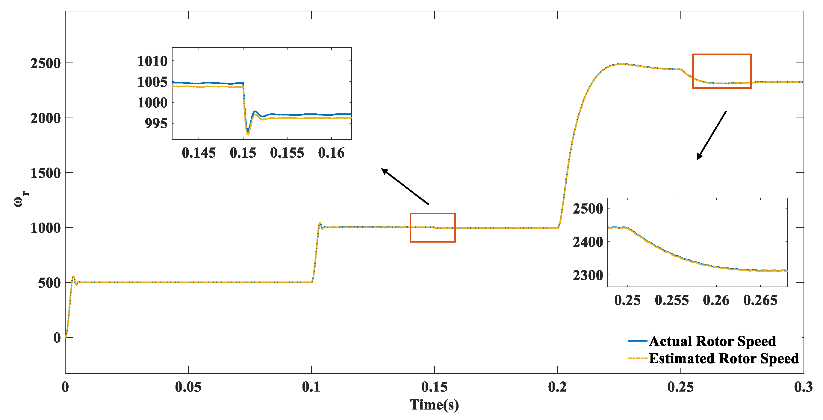
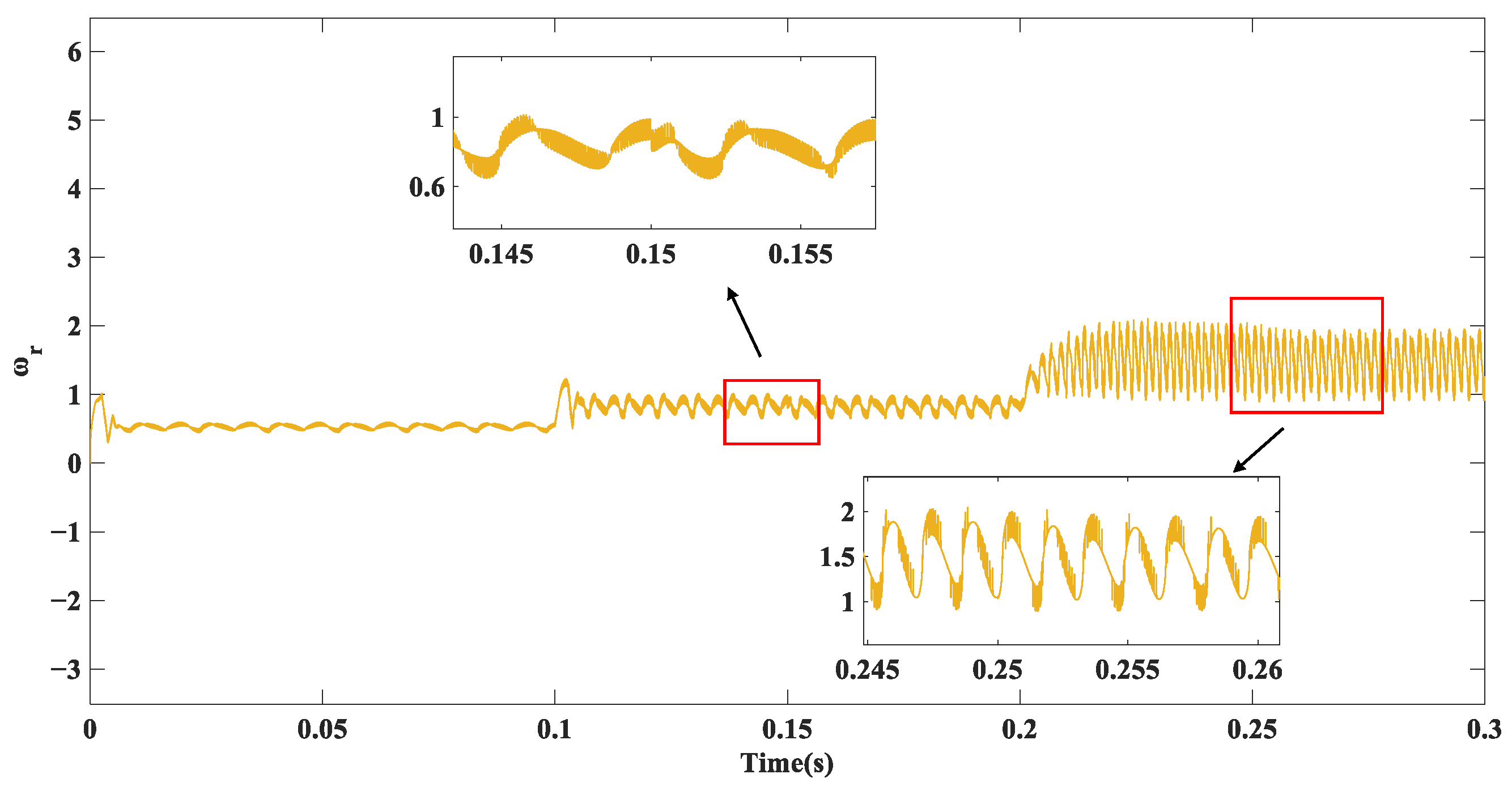
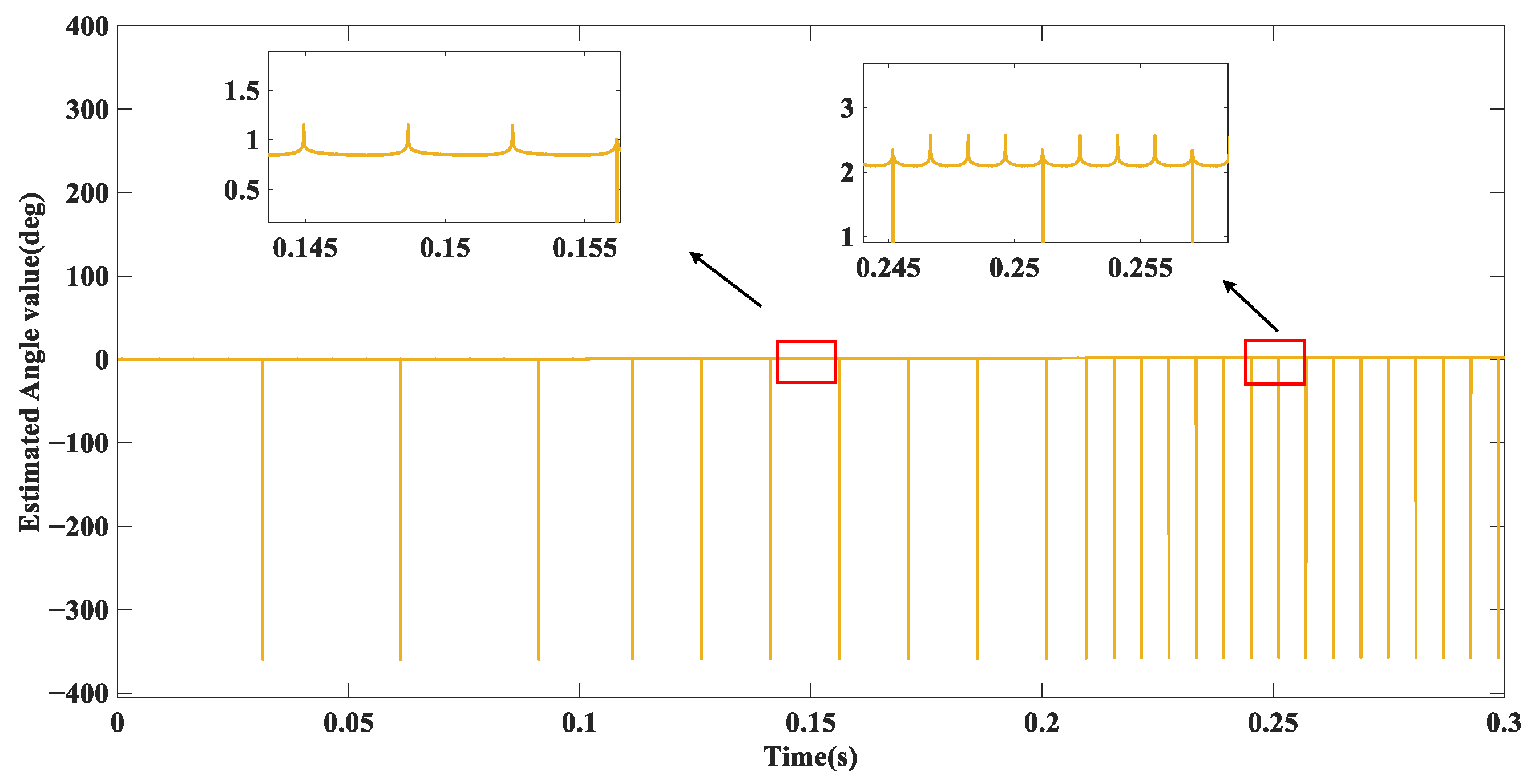
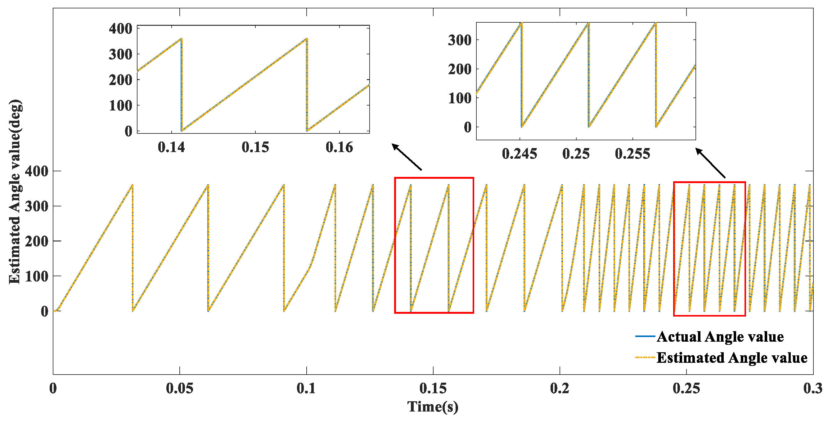
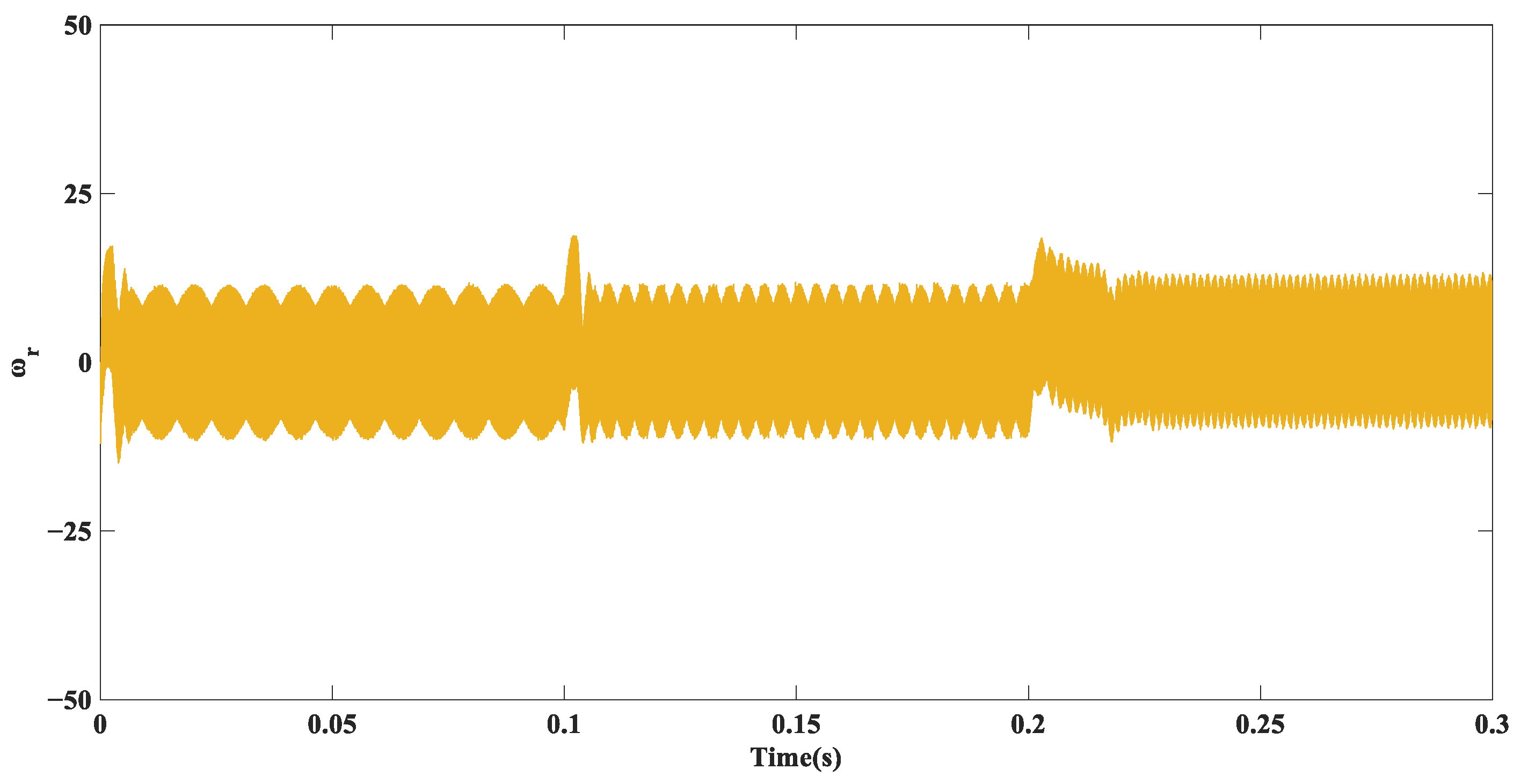
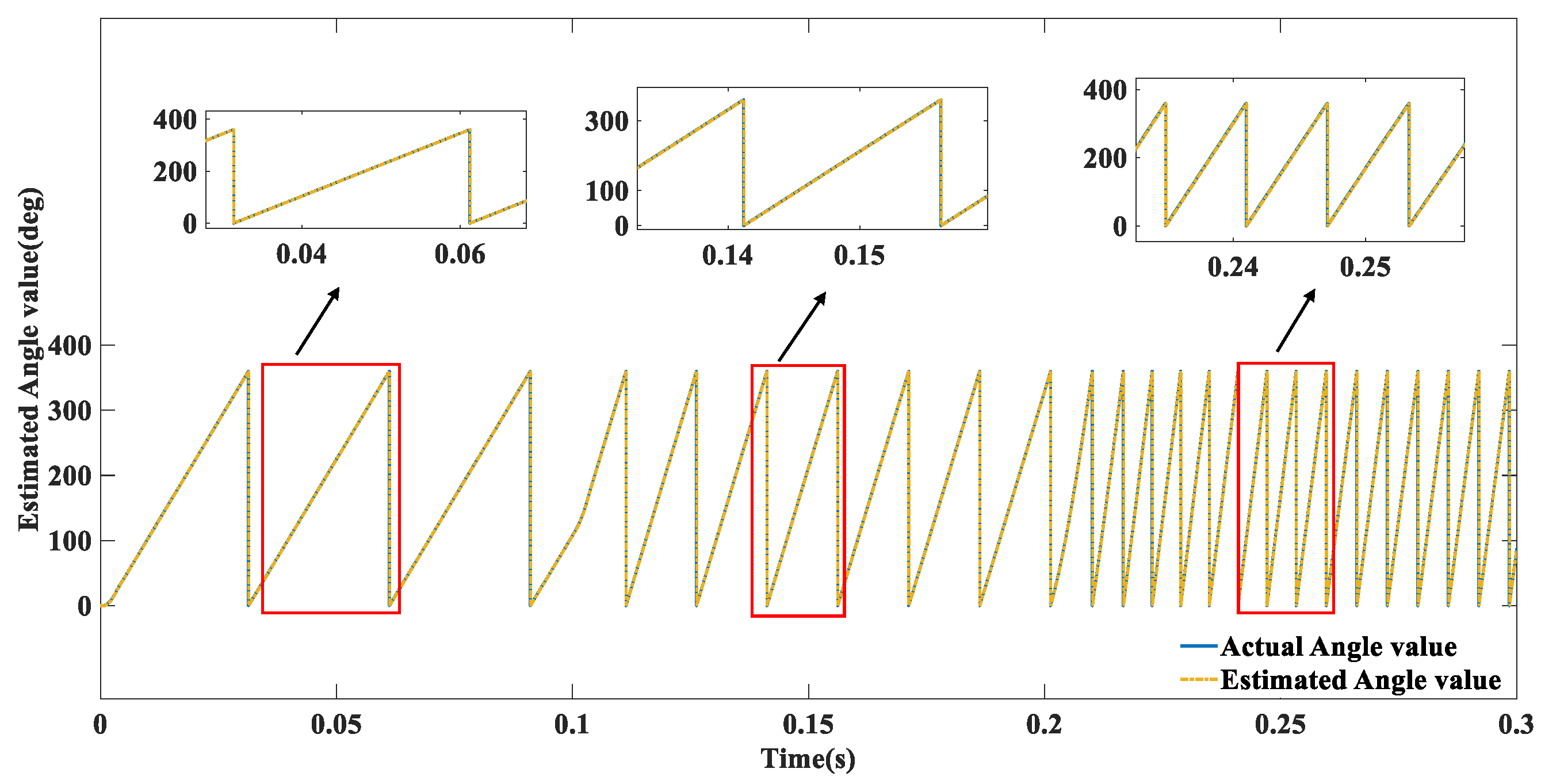
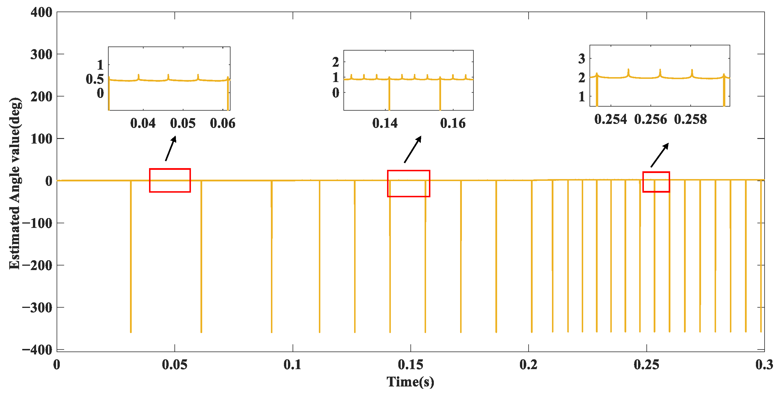
The proposed position-independent observation method is demonstrated by numerical simulation results to effectively reduce buffeting and enhance corresponding speed during speed switching. Validating the system’s stability under load conditions involves subjecting it to different loads at different times.
The rest of this article is arranged in the following manner: Section 2 presents the mathematical model of discrete systems for permanent magnet synchronous motors. The new discrete sliding mode observer’s design methodology is explained in Section 3. The design approach for adaptive phase-locked loops is outlined in Section 4. Our proposed method is verified and validated through the use of MATLAB/Simulink 2022b simulations in Section 5. Finally, Section 6 provides a summary of this thesis.

2. Mathematical Model of a Permanent Magnet Synchronous Motor

To simplify the mathematical model of the PMSM, the motor voltage equation assumes a sinusoidal distribution of the air-gap magnetic field in the α-β axis system while neglecting eddy current and hysteresis losses [19].
u = R s + d L d d t ω e ( L d L q ) ω e ( L d L q ) R s + d L q d t i + e
where u = [uα uβ]T is the stator voltage α-β-axis component; Ld and Lq are the stator inductance d-q-axis components; Rs is the stator resistance; ωe is the electrical angular velocity; i = [iα iβ]T is the stator current α-β-axis component, and e is the expanding counter-potential in the α-β-axis system with the expression:
e = e α e β = ω e ψ f sin θ e ω e ψ f cos θ e
where Ψf is the permanent magnet chain; θe is the electrical angle.
For a table-posted permanent magnet synchronous motor, the stator inductance is approximated by Ld = Lq = Ls. This simplifies and rewrites Equation (1) as the current equation of state.
d i d t = R s L s i + 1 L s u 1 L s e

3. Design of a Sliding Mode Observer for Gain of a Discrete Variable

3.1. Design of a Conventional Super-Twisting Sliding Mode Observer

The Super-Twisting Algorithm–Sliding Mode Observer (STA-SMO) was designed by utilizing a twisting algorithm–sliding mode approach [20], which incorporates nonlinear feedback into the state variables, thereby enabling the system to achieve fast and smooth tracking and control. This algorithm offers high precision and robustness, effectively addressing the buffeting issue encountered in traditional sliding mode control.
The main reason for the chattering of the sliding mode observer is the discontinuity of the control signal, so reducing the chattering allows the signal to become continuous and smooth and have a higher derivative property. Therefore, in order to solve the problem of sign() signal discontinuity at zero time, homogeneous function and integral control are added to the design of traditional super-twisting observers. For example, multiplying a homogeneous function with an absolute value before the sign() function gives us the following equation:
lim x 0 x α s i g n ( x ) = lim x 0 + x α s i g n ( x ) = 0 , α > 0
Another way to solve the chattering problem is to introduce integrals. kp and ki can be designed as follows according to the first-order system model:
k p = k 1 / x 1 x ^ 1 1 / 2
k i = k 2 / x 1 x ^ 1
Therefore, the expression of the super-twisting sliding mode is as follows:
d x ^ 1 d t = k 1 x 1 x ^ 1 x 1 x ^ 1 s i g n ( x 1 x ^ 1 ) + x ^ 2 + p 1 d x ^ 2 d t = k 2 x 1 x ^ 1 x 1 x ^ 1 s i g n ( x 1 x ^ 1 ) + p 2
When the perturbation is ignored, it can be regarded as a linear PI controller with variable gain, whose gain kp and ki change with the absolute value of the state. We can simplify Equation (7) to Equation (8):
d x ^ 1 d t = k 1 x 1 x ^ 1 1 2 s i g n ( x 1 x ^ 1 ) + x ^ 2 + p 1 d x ^ 2 d t = k 2 s i g n ( x 1 x ^ 1 ) + p 2
where x1, x2 are the state variables; x ^ 1 , x ^ 2 is the estimated value of the state variables; k1, k2 are the sliding mode gains; p1, p2 are the perturbation terms.
For any constant ζ greater than zero, the following two equations must hold:
p 1 ζ x 1 1 2 ; p 2 = 0
k 1 > 2 ζ ; k 2 > k 1 5 ζ k 1 + 4 ζ 2 2 ( k 1 2 ζ )
According to the literature [21], the perturbations p1 and p2 in Equation (8) will converge the system to the slip mode surface in finite time if the conditions of Equation (9) are met and the gains k1 and k2 satisfy the conditions of Equation (10).
From Equation (3), the estimated equation for the current in the α-β axis system is given as follows:
d i ^ d t = R s L s i ^ + 1 L s u 1 L s e ^
where i ^ is the observed current in the α-β axis system and e ^ is the observed counter-potential.
The current error equation is obtained by subtracting Equation (3) from Equation (11).
d i ˜ d t = R s L s i ˜ 1 L s ( e ^ e )
where i ˜ = i ^ i is the observed error value of the stator current.
When the current observation error converges and i ˜ = 0, the observed value of the anti-potential equals the actual value. The estimated value of the anti-potential, designed based on the super-twisting algorithm, is:
e ^ = k 1 i ˜ 1 2 s i g n ( i ˜ ) k 2 s i g n ( i ˜ ) d t
The initial term of Equation (13) will gradually decrease as the current error converges.
By comparing Equations (8) and (11), we can obtain the current estimation equation as follows:
d i ^ d t = k 1 L s i ˜ 1 2 s i g n ( i ˜ ) k 2 L s s i g n ( i ˜ ) d t R s L s i ^ + 1 L s u
The current error equation can be obtained by subtracting Equation (3) from Equation (14).
d i ˜ d t = k 1 L s i ˜ 1 2 s i g n ( i ˜ ) k 2 L s s i g n ( i ˜ ) d t R s L s i ˜ + 1 L s e
When the system achieves stability, the estimation error is on the sliding mode surface. This indicates that the estimated value is close to the actual value, and the rotor position can then be estimated using Equation (15). Due to the discontinuity of the sign function in practical applications, the estimated current switches back and forth on the sliding mode surface, resulting in a noticeable jittering phenomenon. In this paper, we propose a discrete variable gain super-twisting sliding mode observer that can adjust the convergence function based on the rotational speed.

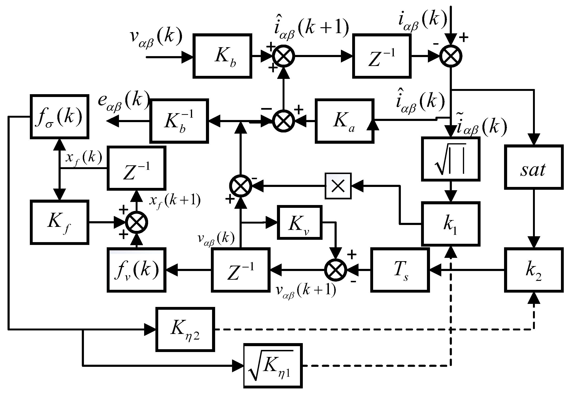
3.2. Design of a Sliding Mode Observer for Discrete Variable Gain

In computerized control systems, continuous systems need to be discretized. According to the article [22], Equation (3) is discretized and expressed by Equation (16):
i ( k + 1 ) = ( 1 T s R s L s ) i ( k ) + T s L s u ( k ) e ( k )
where k is the sampling moment; i(k), u(k), and e(k) are the current, voltage, and anti-potential values at moment k, respectively; and Ts is the discrete system sampling period.
To obtain anti-potential estimates, a sliding mode observer with perturbation observation compensation is designed. The current state Equation (16) is revised to remove anti-potential information.
i ^ ( k + 1 ) = ( 1 T s R s L s ) i ^ ( k ) + T s L s u ( k ) δ ( k )
where i ^ is the observed value of the stator current, δ is a parameter containing an estimate of the counter potential, and δ(k) is defined as follows:
δ ( k ) = v ( k ) k 1 ( k ) i ˜ ( k ) s a t ( i ˜ ( k ) )
v ( k + 1 ) = K v v ( k ) T s k 2 ( k ) s a t ( i ˜ ( k ) )
where i ˜ is the stator current observation error and its expression is as follows:
i ˜ ( k ) = i ( k ) i ^ ( k )
The constant Kv is a fixed value that always satisfies 0 < Kv < 1. The auxiliary gain, v(k), is used in conjunction with the sat(s) function, which is defined as follows:
s a t ( s ) = 1 s 1 c arctan ( q s c ) s < 1 c 1 s 1 c
where q = tan(1) = 1.557, c is the sliding mode boundary and s is the sliding mode surface. k1(k), k2(k) functions are defined as follows:
k 1 ( k ) = K η 1 f σ ( k )
k 2 ( k ) = K η 2 f σ ( k )
Kη1 and Kη2 are constants. The function fσ(k) is bounded and defined as follows:
f σ ( k ) = σ min 0 σ ( k ) < σ min σ ( k ) σ min σ ( k ) < σ max σ max σ ( k ) > σ max
where σmin, σmax, σ(k) are defined as follows.
σ max = T s L s λ p m ω max
σ min = T s L s λ p m ω min
σ ( k ) = ( 1 K f ) x f ( k )
where λpm is the permanent magnet magnetic chain, ωmax and ωmin are the maximum and minimum electrical angular velocities during motor operation [23], xf is the low-pass filter state parameter; Kf is the low-pass filter gain, and the expression is as follows:
K f = e ω f T s
where ωf is the filter cutoff frequency.
Then, the filter dynamic equation is:
x f ( k + 1 ) = K f x f ( k ) + f v ( k )
where fv(k) is defined as follows:
f v ( k ) = v ( k ) 0 < v ( k ) < v max v max v ( k ) > v max
where vmax = σmax.
In summary, Figure 1 shows the structure of the new discrete variable gain sliding mode observer.

3.3. Feasibility and Convergence Analysis

3.3.1. Proof of Feasibility

The feasibility of Equation (18) is analyzed and proved as follows:
From Equation (20):
i ˜ ( k + 1 ) = i ( k + 1 ) i ^ ( k + 1 )
By substituting Equations (16) and (17) into Equation (31), the following is obtained:
i ˜ ( k + 1 ) = K a i ˜ ( k ) K b e ( k ) + δ ( k )
where K a = 1 T s R s L s , K b = T s L s .
We can assume the existence of an ideal sliding mold surface that satisfies Equation (33).
i ˜ ( k + 1 ) = i ˜ ( k ) = 0
Substituting Equation (33) into Equation (31) gives the following:
δ ( k ) = K b e ( k )
Assuming the existence of an ideal slip mold surface, Equation (18) can be rewritten as follows:
δ ( k ) = v ( k )
It is possible to request the following:
v ( k ) = K b e ( k )
The e(k) counter-potential is proportional to the rotor speed, and therefore, v(k) is also proportional to the rotor speed. As fv(k) is a function of v(k), it can be concluded that fv(k) is also proportional to the rotor rotational speed. This allows for the rotor rotational speed to be used in fv(k) to calculate the gain coefficients, k1(k) and k2(k), of the discrete sliding mode observer Equation (18) in real-time, achieving discrete variable gain sliding mode observation of the counter-potential.
The counter-potential can be estimated directly from Equation (34).
e ^ ( k ) K b 1 δ ( k )
Equations (18) and (32) provide the necessary information.
i ˜ ( k + 1 ) = K a i ˜ ( k ) K b e ( k ) + v ( k ) k 1 ( k ) i ˜ ( k ) s a t ( i ˜ ( k ) )
The equation above describes the updated law of the sliding mode controller in discrete time. Control input is calculated based on the current state of the sliding mode, and the sliding mode surface is updated accordingly to achieve system control through continuous iterative calculation. Equation (38) shows that Ka controls the update rate of the sliding mode surface, while Kb controls the error decay rate.
The analysis above demonstrates that the switching function trajectories described in Equations (12) and (31) always converge to the quasi-smooth mode surface of i ˜ ( k ) ε , provided that the perturbation Kbe(k) is bounded and there exists a value of 0 < Ka < 1 such that k1(k), k2(k), and Kv satisfy 0 < k1(k) ≤ Kη1(σmax)½, 0 < k2(k) ≤ Kη2σmax, and 0 < Kv < 1, respectively.

3.3.2. Proof of Convergence

The feasibility of the new discrete variable gain super-twisting sliding mode observer has been demonstrated through the above analysis. Next, its convergence is analyzed using the inverse method. It is assumed that the trajectory of the switching function deviates from the sliding surface, which is obtained by subtracting i ˜ ( k ) on both sides of Equation (38), respectively.
i ˜ ( k + 1 ) i ˜ ( k ) = ( 1 K a ) i ˜ ( k ) K b e ( k ) + v ( k ) k 1 ( k ) i ˜ ( k ) s a t ( i ˜ ( k ) )
Assuming that i ˜ ( k ) + , i ˜ ( k ) > 0 , we obtain the following:
i ˜ ( k + 1 ) i ˜ ( k ) > 0
By substituting Equation (40) into Equation (39), we obtain:
v ( k ) K b e ( k ) > ( 1 K a ) i ˜ ( k ) + k 1 ( k ) i ˜ ( k ) s a t ( i ˜ ( k ) )
If i ˜ ( k ) + , it can be seen that v ( k ) . Equation (42) is satisfied when k ≥ N such that i ˜ ( k + 1 ) i ˜ ( k ) < 0 , and the convergence condition is met.
v ( k ) K b e ( k ) < ( 1 K a ) i ˜ ( k ) + k 1 ( k ) i ˜ ( k ) s a t ( i ˜ ( k ) )
Therefore, the above assumption that the trajectory of the switching function deviates from the sliding surface does not hold, showing that when i ˜ ( k ) + , i ˜ ( k ) < 0 . Similarly, it can be shown that when i ˜ ( k ) , i ˜ ( k ) < 0 does not hold. In other words, when k→∞, the trajectory of the switching function does not deviate from the sliding surface, and when the stator current error tends to 0, v(k) ≈ Kbe(k).
From Equation (33) and Equation (34), the conditions for the motion of the switching function on the surface of the sliding mold are as follows:
v ( k ) = K b e ( k ) v ( k + 1 ) = K b e ( k + 1 ) e ( k + 1 ) = K v e ( k )
When the stator current error tends to 0, the expression for v(k) is obtained:
v ( k ) K b e ( k ) + i ˜ ( k )
where v ˜ ( k ) K b ( e ( k ) K v e ( k 1 ) ) T s k 2 ( k ) s a t ( i ˜ ( k ) ) ; since Kbe(k) is bounded, v ˜ ( k ) is also bounded and can compensate for the error in the counter-potential estimation.
This can be obtained by substituting K c = K b e ( k ) + v ( k ) , K d = ( 1 K a ) i ˜ ( k ) + k 1 ( k ) i ˜ ( k ) into Equation (32):
i ˜ ( k + 1 ) i ˜ ( k ) = K d s a t ( i ˜ ( k ) ) + K c
Since 1 − Ka > 0 and k1(k) > 0, Kd > 0, i ˜ ( k ) 0 and when kN, K c = v ˜ ( k ) , so the slip mode surface expression is:
i ˜ ( k + 1 ) i ˜ ( k ) = K d s a t ( i ˜ ( k ) ) + v ˜ ( k )
Thus, when k is greater than or equal to N, the equations of motion for the sliding mode are always limited to ε, ensuring convergence.
The block diagram of the PMSM system based on the above variable gain super-twisting sliding mode is shown in Figure 2. In Figure 2, ud* and uq* are the voltage estimates of the d-q-axis obtained through the PI controller, while uα* and uβ* are the voltage estimates under the α-β-axis obtained through the Park transformation of ud* and uq*. These values are used to calculate the sliding mode parameters in the next period.

4. Phase-Locked Loop Performance Improvement

The study focuses on position sensor-less control of permanent magnet synchronous motors. The rotor position can be calculated directly using the inverse tangent method by utilizing the counter-potential estimated by a sliding mode observer [24]. However, in practice, the magnetic chain of a motor cannot be directly measured. It can only be estimated based on a motor model, which inevitably introduces some degree of error. Additionally, the sliding mode observer switching function causes high-frequency dithering in the estimated counter-potential. To mitigate this issue, a low-pass filter [25] is necessary, but it can introduce unwanted errors. To improve the accuracy of rotor position observation, this paper proposes an adaptive quadrature phase-locked loop method to compensate for these errors.

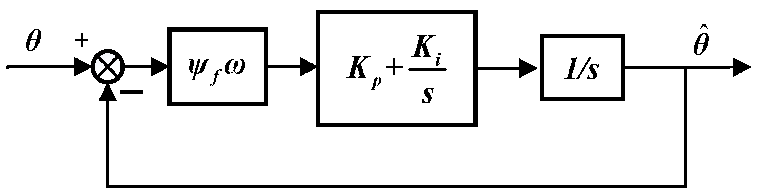
4.1. Design and Analysis of Basic Phase-Locked Loop

Figure 3 shows the structure of the phase-locked loop (PLL) for a permanent magnet synchronous motor in the α-β axis system [26].
For ω ^ , θ ^ is the estimated value of the motor rotor position and Δu is expressed as follows:
Δ u = e ^ α cos θ e ^ β sin θ
Substituting Equation (47) into Equation (2) gives:
Δ u = ψ f ω sin θ ^ cos θ ψ f ω cos θ ^ sin θ = ψ f ω sin ( θ θ ^ )
When the PI controller adjusts Δu to θ = θ ^ , it becomes possible to calculate the estimated position of the rotor [27]. The process of parameterizing Kp and Ki in the PI controller is as follows:
When θ θ ^ is approximately equal to 0, the PLL structure diagram shown in Figure 3 can be simplified to Figure 4.
In Figure 4, the open-loop transfer function is:
G ( s ) = ψ f G ( K p + K i s ) 1 s = ψ s ω ( K p s + K i ) s 2
The closed-loop transfer function is:
Φ ( s ) = ψ f ω K p s + ψ f ω K i s 2 + ψ f ω K p s + ψ f ω K i
The typical form of a second-order system is determined by taking this as the tuning parameter.
G ( s ) = ω n 2 s 2 + 2 ξ ω n s + ω n 2
The closed-loop transfer function can be calculated using the standard form of a second-order system, resulting in the following equation.
ψ f ω K p = 2 ξ ω n ψ f ω K i = ω n 2
Kp and Ki can be calculated from Equation (52).

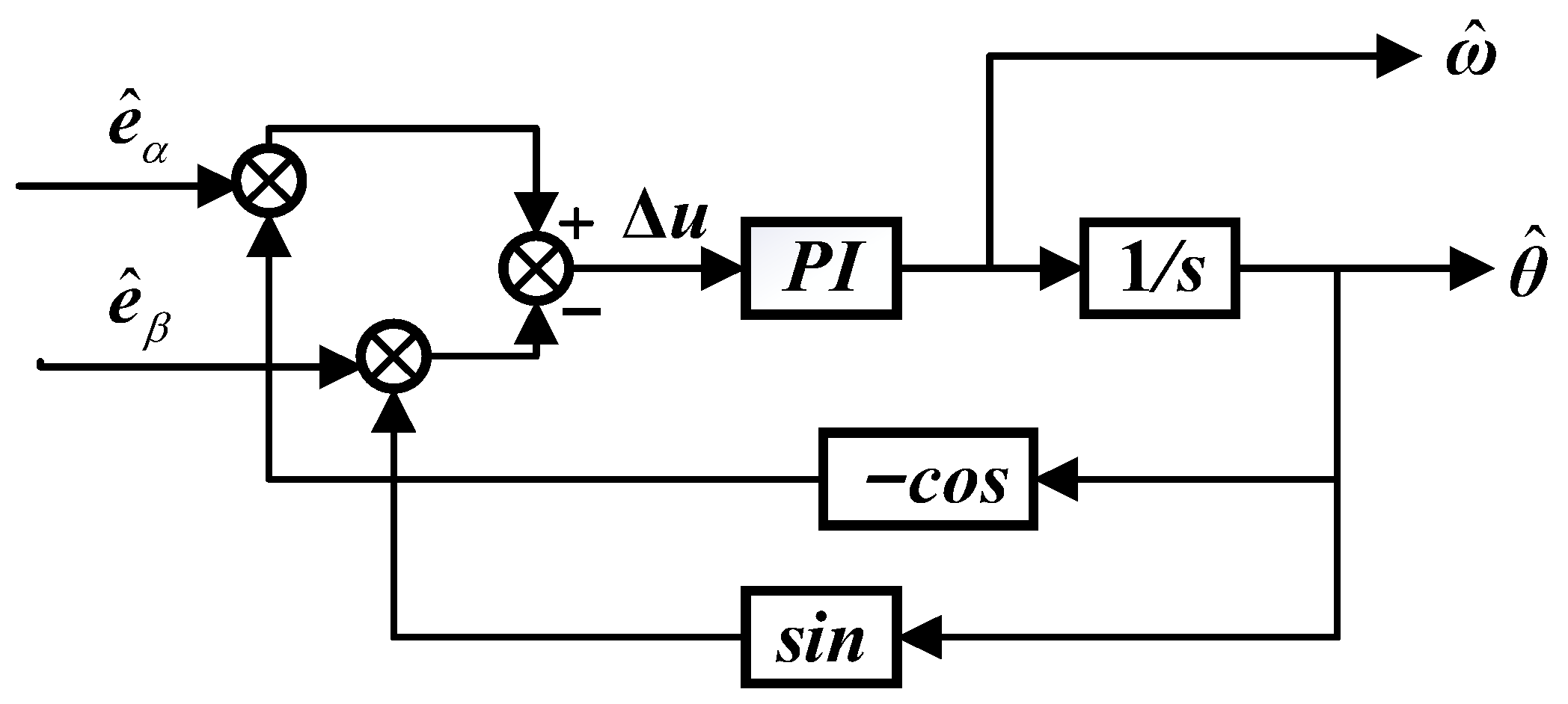
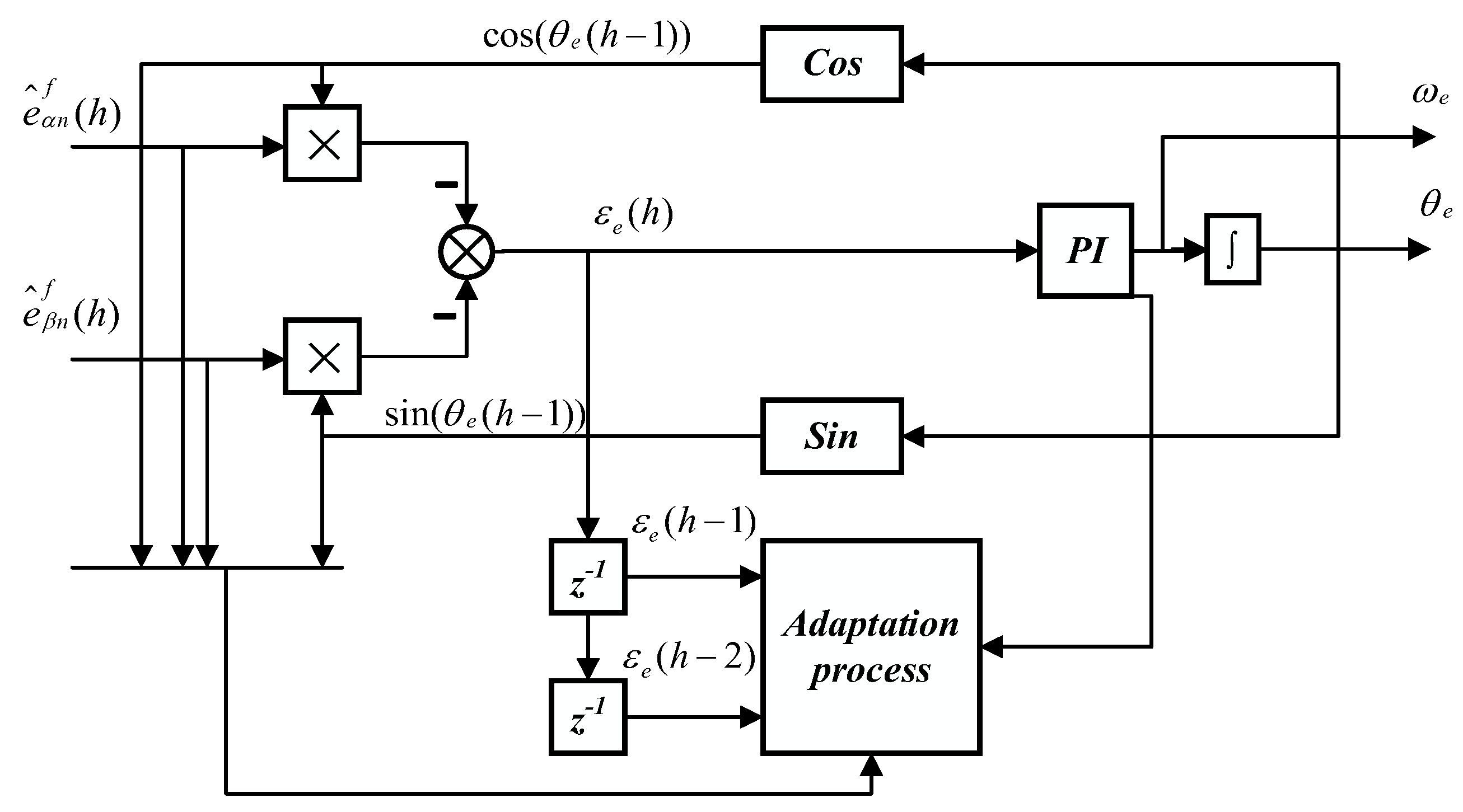
4.2. Design of Adaptive Quadrature Phase-Locked Loop

In the control system depicted in Figure 2, the counter-potential obtained through estimation by a discrete variable gain sliding mode observer is fed into the quadrature phase-locked loop (QPLL) for rotor position calculation [28]. Compared to a basic phase-locked loop with a fixed bandwidth, the adaptive quadrature phase-locked loop can dynamically adjust its bandwidth based on the rotational speed of the motor [29]. This adjustment effectively reduces estimation errors in the rotor position and enhances accuracy in rotor position estimation, thereby enabling proper decoupling of rotor current and resulting in higher torque output [30]. As illustrated in Figure 5, when feeding estimated anti-potential information into the adaptive quadrature phase-locked loop, an adaptive filter needs to be incorporated to eliminate harmonic components present in the anti-potential information. The transfer function of this quadrature phase-locked loop is as follows:
G P L L ( s ) = e ^ k p s + e ^ k i s 2 + e ^ k p s + e ^ k i
In order to reduce the error of the back EMF, the back EMF can be normalized by Equation (54).
e ^ = e ^ / e ^ α 2 + e ^ β 2
After normalizing the inverse potential, the bandwidth of the quadrature phase-locked loop is no longer affected by the rotor speed [31]. As a result, the transfer function can be simplified as:
G P L L ( s ) = k p s + k i s 2 + k p s + k i
We can replace the poles in Equation (55) with Equation (56) as follows:
k p ( h ) = 2 τ ρ ( h ) k i ( h ) = ρ 2 ( h )
where τ is the damping coefficient; ρ is the AQPLL tuning parameter; h is the discrete time step parameter.
Because it is difficult to adjust both τ and ρ at the same time and the bandwidth of the QPLL is related to ρ, the damping coefficient is set to a constant value in order to simplify the calculation process. The AQPLL tuning parameter ρ is set as follows:
ρ ( h ) = ρ ( h 1 ) μ 1 2 ( ε e ( h ) h ( h 1 ) )
where μ is the step parameter of the adaptive speed and εe is the PI controller input error of the QPLL.
The final equation for updating the tuning parameters can be expressed as:
ρ ( h ) = ρ ( h 1 ) μ z 1 ( h ) z 2 ( h ) = ρ ( h 1 ) Δ ρ ( h )
where z1 and z2 parameters are set as follows:
z 1 ( h ) = e ^ α n f ( h ) sin ( θ ^ e ( h 1 ) ) e ^ β n f ( h ) cos ( θ ^ e ( h 1 ) ) z 2 ( h ) = 2 τ ε e ( h 1 ) + T s p ( h 1 ) ( ε e ( h 1 ) ε e ( h 2 ) )
where e ^ α n f , e ^ β n f is the filtered counter-potential estimate.
The AQPLL logic block diagram designed based on the above analysis is shown in Figure 6.

4.3. Stability Analysis

To analyze the stability of AQPLL as ρ varies, we use Equation (56) in Equation (55) to calculate the root of the AQPLL characteristic equation.
s 1 , 2 = τ ρ ± ρ ( τ 2 1 )
According to the literature [32], the roots of the characteristic equation remain in the left half-s plane as long as ρ > 0, indicating stability of the AQPLL system. It is difficult to observe the counter-potential accurately when the motor is running at lower speeds, so it is necessary to limit the minimum speed of the motor, i.e., the value of ρ:
ρ ρ min
where ρmin is the minimum value of ρ that can lock the motor frequency during motor startup.
The computation of the observer gain is only possible if the observer’s dynamic response is faster than the PMSM state change. Additionally, the observer gain is limited by the observer state feedback [33].
x ^ ˙ α β = ( A ( ω ^ e ) K C ) x ^ α β + B v α β * + K i ˜ α β
where the matrix expression for C is 1 0 0 0 0 1 0 0 ; x ^ α β is the observer gain.
Note that the observer gain in Equation (62) must be valid for the entire speed range of the motor and the closed-loop poles must remain in the left half-s plane [34].

5. Simulation Experiments

In order to verify the effectiveness of the proposed method, fixed gain and variable gain super-torsional sliding mode observers were constructed in MATLAB/Simulink, as shown in Figure 2. The adaptive orthogonal phase-locked loop (PLL) method is used to obtain the rotor position of both observers, and a PI controller is used in the speed loop of the motor control system. Simulation experiment parameters are shown in the following table. The horizontal coordinate in the figure below represents the time used in the simulation, and the vertical coordinate represents the rotor speed comparison, rotor speed error, rotor position comparison, and rotor position error.
Table 1 includes the values of the parameters used in the experiment: Rs represents the stator resistance of the motor; VDC indicates the voltage level of the motor; Ls denotes the stator inductance; ωrmax signifies the maximum allowable speed of the motor; power refers to the power supply’s output. Ts represents the sampling period. Kη1, Kη2, and Kv are constants; ωc is defined as the cut-off frequency; λpm represents a permanent magnet flux linkage; J stands for moment of inertia; pole pairs indicate the number of poles present in the motor structure; B represents magnetic induction intensity. ωr denotes motor speed, while ωf signifies the filter cut-off frequency. Q is used to represent the quality factor.
Figure 7 shows the actual versus estimated speed waveforms of the output of the fixed gain super-twisting sliding mode observer for an initial speed of 500 r/min at no load on the motor, 1000 r/min given at 0.1 s, and 2500 r/min at 0.2 s. The output of the fixed gain super-twisting sliding mode observer is shown in Figure 8, which shows the actual versus estimated speed waveforms.
Figure 7 and Figure 8 show that when fixed gain STA-SMO is used, the speed error remains around 10 r/min because the fixed gain sliding mode parameter is calculated based on the maximum and minimum speed of the rotor, so the speed error does not fluctuate much when the speed varies.
Figure 9 and Figure 10 show the estimated rotor position and the actual rotor position information when the fixed gain sliding mode observer is used. From the figure, it can be seen that the rotor position error increases as the motor speed increases.
The actual speed exhibits a slight decrease relative to the reference speed when different loads are added at 0.15 s and 0.25 s, as depicted in Figure 11 and Figure 12, respectively; however, the error between the estimated speed and the actual speed remains constant at 10 r/min.
The waveforms of the estimated rotor position and the actual rotor position with loads, along with their corresponding position errors, are depicted in Figure 13 and Figure 14. The obtained results indicate that under different load conditions, when estimating the rotor position using a fixed gain approach, the position error is approximately 2 radians at 0.15 s and around 4 radians at 0.25 s.
Figure 15 and Figure 16 show the motor speed and the actual speed information estimated using the variable gain super-twisting sliding mode observer for a given speed variation when the motor is unloaded.
As shown in Figure 15, the variable gain super-twisting sliding mode observer not only eliminates the high-frequency jittering observed in Figure 7, but also results in improved convergence of the estimates to the true values. As can be seen from the enlarged view of Figure 16, the maximum error is only 0.6 r/min when the given speed is 500 r/min. When the 0.1 s speed is 1000 r/min, the speed error is only 1 r/min. And when the motor is in the high-speed domain at 2500 r/min, the speed error is only 2 r/min.
From Figure 17 and Figure 18, it can be seen that the rotor position error is always kept small when the rotational speed is at 500 r/min, 1000 r/min, and 2500 r/min, respectively.
From the comparison between Figure 10 and Figure 18, it can be seen that the rotor position estimation accuracy is higher and the position estimation error is reduced by half when the variable gain super-twisting sliding mode observer is used.
To verify the stability of the variable gain super-twisting sliding mode observer with load, a load of 4 N-M was added at 0.15 s and raised to 10 N-M at 0.25 s. The rotational speed and positional errors were observed for a given constant rotational speed.
From Figure 19, it can be seen that the estimated and actual speed decreases by 10 r/min when the load is applied suddenly at 0.15 s and stabilizes to 998 r/min at 0.152 s. Likewise, when the load is abruptly increased at 0.25 s, the speed will decrease by 150 revolutions per minute and will stabilize after 0.01 s. From Figure 20 and Figure 21 it can be seen that sudden loading has no effect on the speed error and rotor position error, which also shows the observation accuracy of this observer with a load.
Figure 20 and Figure 22 Everyone has agreed demonstrate the performance of the variable gain STA-SMO under loads. The variable gain module reacts quickly to sudden load additions at 0.15 s and 0.25 s by adjusting the sliding mode control rate in real-time based on the rotor speed change. The simulation results show that the variable gain STA-SMO can accurately estimate the rotor speed and position under various operating conditions of the motor.

6. Conclusions

A sensor-less estimation method of a permanent magnet synchronous motor based on a discrete variable gain super-twisting sliding mode observer and adaptive orthogonal phase-locked loop is proposed. The signal estimated by the discrete variable gain super-twisting sliding mode observer can effectively avoid buffering, and can quickly track the rotor speed and position in real time, so as to minimize the error between the actual value and the estimated value. The parameters in the adaptive orthogonal PLL can also be adjusted according to the motion state of the rotor, which effectively improves the problem of the poor tracking performance of the rotor caused by the fixed bandwidth in the traditional PLL. The simulation results show that the speed error of the fixed gain observer is about 10 r/min when the speed is 500 r/min, 1000 r/min and 2500 r/min, while the speed error of the variable gain observer is only 1 r/min. Therefore, the performance of the variable gain observer in rotor speed estimation is better than that of the fixed gain observer. In terms of rotor position estimation, the rotor position error shown by the variable gain observer is only half that of the fixed gain observer. Moreover, when the system speed is switched, the response time required by the variable gain observer is shorter and closer to the actual situation. In order to further study the observation of the proposed estimation method under loads, different loads were added at 0.15 s and 0.25 s, respectively. The simulation results show that under the influence of a load, the estimated performance of rotor speed and position is not weakened, and the error between the estimated value and the actual value is the same as that when the load is 0, so the rotor position can be controlled with high precision.

Author Contributions

Algorithm design, M.L.; coding and testing, M.L; mathematical derivation, M.L. and Y.Z.; article review and proofreading, X.L.; funding acquisition, X.L. and F.X. All authors have read and agreed to the published version of the manuscript.

Funding

This work was supported by the Science and Technology Major Project of Inner Mongolia Autonomous Region (2020ZD0014).

Institutional Review Board Statement

Not applicable.

Informed Consent Statement

Not applicable.

Data Availability Statement

The original contributions presented in the study are included in the article, further inquiries can be directed to the corresponding author.

Acknowledgments

We would like to acknowledge the School of Rail Transportation of Shandong Jiaotong University for providing the experimental equipment and assistance with the experimental testing.

Conflicts of Interest

The authors declare no conflicts of interest.

References

  1. Yu, B.; Shen, A.; Chen, B.; Luo, X.; Tang, Q.; Xu, J.; Zhu, M. A compensation strategy of flux linkage observer in SPMSM sensor-less drives based on linear extended state observer. IEEE Trans. Energy Convers. 2021, 37, 824–831. [Google Scholar] [CrossRef]
  2. Yang, Y. Research on Position Sensor-Less Control System of Permanent Magnet Synchronous Motor; Harbin Institute of Technology: Harbin, China, 2018. [Google Scholar]
  3. Shen, Y.; Liu, A.; Cui, G.; Yang, X.; Zheng, Z. Sensor-less vector control of permanent magnet synchronous motor with extended sliding mode observer. J. Electr. Mach. Control. 2020, 24, 8. [Google Scholar] [CrossRef]
  4. Volpato Filho, C.J.; Xiao, D.; Vieira, R.P.; Emadi, A. Observers for high-speed sensor-less pmsm drives: Design methods, tuning challenges and future trends. IEEE Access 2021, 9, 56397–56415. [Google Scholar] [CrossRef]
  5. Wu, Z.; Li, R. Sensor-less control of PMSM based on sliding mode variable structure control and adaptive sliding mode observer. In Proceedings of the 2021 24th International Conference on Electrical Machines and Systems (ICEMS), Gyeongju, Republic of Korea, 31 October–3 November 2021; pp. 2015–2019. [Google Scholar]
  6. Zribi, M.; Chiasson, J. Position control of a PM stepper motor by exact linearization. IEEE Trans. Autom. Control 1991, 36, 620–625. [Google Scholar] [CrossRef]
  7. Yao, Y.; Huang, Y.; Peng, F.; Dong, J.; Zhu, Z. Compensation method of position estimation error for high-speed surface-mounted PMSM drives based on robust inductance estimation. IEEE Trans. Power Electron. 2021, 37, 2033–2044. [Google Scholar] [CrossRef]
  8. Tang, Q.; Yu, B.; Luo, P.; Luo, X.; Shen, A.; Xia, Y.; Xu, J. Second Harmonic Seamless Splicing Technique Based on Maximum Active-Voltage Vector for Online MTPA Tracking Control of SynRM. IEEE Trans. Ind. Electron. 2021, 69, 10958–10968. [Google Scholar] [CrossRef]
  9. Luo, X.; Shen, A.; Tang, Q.; Liu, J.; Xu, J. Two-step continuous-control set model predictive current control strategy for SPMSM sensor-less drives. IEEE Trans. Energy Convers. 2020, 36, 1110–1120. [Google Scholar] [CrossRef]
  10. Ding, S.; Hou, Q.; Wang, H. Disturbance-observer-based second-order sliding mode controller for speed control of PMSM drives. IEEE Trans. Energy Convers. 2022, 38, 100–110. [Google Scholar] [CrossRef]
  11. Wang, M.; Sun, D.; Zheng, Z.; Nian, H. A novel lookup table based direct torque control for OW-PMSM drives. IEEE Trans. Ind. Electron. 2020, 68, 10316–10320. [Google Scholar] [CrossRef]
  12. Xiong, Y.; Wang, A.; Zhang, T. Sensor-Less Complex System Control of PMSM Based on Improved SMO. In Proceedings of the 2021 6th International Conference on Automation, Control and Robotics Engineering (CACRE), Dalian, China, 15–17 July 2021; pp. 228–232. [Google Scholar]
  13. Guo, L.; Wang, H.; Jin, N.; Dai, L.; Cao, L.; Luo, K. A speed sensor-less control method for permanent magnet synchronous motor based on super-twisting sliding mode observer. In Proceedings of the 2019 14th IEEE Conference on Industrial Electronics and Applications (ICIEA), Xi’an, China, 19–21 June 2019; pp. 1179–1184. [Google Scholar]
  14. Zhang, J.; Tian, J.; Alcaide, A.M.; Leon, J.I.; Vazquez, S.; Franquelo, L.G.; Luo, H.; Yin, S. Lifetime Extension Approach Based on Levenberg-Marquardt Neural Network and Power Routing of DC-DC Converters. IEEE Trans. Power Electron. 2023, 38, 10280–10291. [Google Scholar] [CrossRef]
  15. Ke, W.; Sun, D.; Zhang, X.; Nian, H.; Hu, B. Adaptive Capacitor Voltage-Based Model Predictive Control for Open-Winding PMSM System with a Floating Capacitor. IEEE J. Emerg. Sel. Top. Power Electron. 2022, 11, 442–452. [Google Scholar] [CrossRef]
  16. Sun, C.; Sun, D.; Chen, W.; Nian, H. Improved model predictive control with new cost function for hybrid-inverter open-winding PMSM system based on energy storage model. IEEE Trans. Power Electron. 2021, 36, 10705–10715. [Google Scholar] [CrossRef]
  17. Chen, W.; Sun, D.; Wang, M.; Nian, H. Modeling and control for open-winding PMSM under open-phase fault based on new coordinate transformations. IEEE Trans. Power Electron. 2020, 36, 6892–6902. [Google Scholar] [CrossRef]
  18. Wang, M.; Sun, D.; Ke, W.; Nian, H. A universal lookup table-based direct torque control for OW-PMSM drives. IEEE Trans. Power Electron. 2020, 36, 6188–6191. [Google Scholar] [CrossRef]
  19. Sun, D.; Chen, W.; Cheng, Y.; Nian, H. Improved direct torque control for open-winding PMSM system considering zero-sequence current suppression with low switching frequency. IEEE Trans. Power Electron. 2020, 36, 4440–4451. [Google Scholar] [CrossRef]
  20. Zheng, Z.; Sun, D.; Wang, M.; Nian, H. A dual two-vector-based model predictive flux control with field-weakening operation for OW-PMSM drives. IEEE Trans. Power Electron. 2020, 36, 2191–2200. [Google Scholar] [CrossRef]
  21. Hu, W.; Ruan, C.; Nian, H.; Sun, D. An improved modulation technique with minimum switching actions within one PWM cycle for open-end winding PMSM system with isolated DC bus. IEEE Trans. Ind. Electron. 2019, 67, 4259–4264. [Google Scholar] [CrossRef]
  22. Cheng, Y.; Sun, D.; Chen, W.; Nian, H. Model predictive current control for an open-winding PMSM system with a common DC bus in 3-D space. IEEE Trans. Power Electron. 2020, 35, 9597–9607. [Google Scholar] [CrossRef]
  23. Zheng, Z.; Sun, D.; Wang, M.; Nian, H. Model predictive control with a novel cost function evaluation scheme for OW-PMSM drives. Electron. Lett. 2020, 56, 655–657. [Google Scholar] [CrossRef]
  24. Zheng, Z.; Sun, D. Model predictive flux control with cost function-based field weakening strategy for permanent magnet synchronous motor. IEEE Trans. Power Electron. 2019, 35, 2151–2159. [Google Scholar] [CrossRef]
  25. Zhou, Q.; Wang, Y.; Shi, K.; Zhang, F.; Du, H. High-frequency pulsating voltage injection PMSM position sensor-less control based on generalized second-order integrator. J. Electr. Mach. Control 2023, 1–10. [Google Scholar]
  26. Chen, B. Research on Medium and High Speed Control Technology and Starting Strategy of Permanent Magnet Synchronous Motor without Position Sensor; Huazhong University of Science and Technology: Wuhan, China, 2021. [Google Scholar]
  27. Liu, G.; Zhang, H.; Song, X. Position-estimation deviation-suppression technology of PMSM combining phase self-compensation SMO and feed-forward PLL. IEEE J. Emerg. Sel. Top. Power Electron. 2020, 9, 335–344. [Google Scholar] [CrossRef]
  28. Chen, S. Research on Position Sensor-Less Control Strategy of Permanent Magnet Synchronous Motor in Full Speed Domain; China University of Mining and Technology: Beijing, China, 2020. [Google Scholar]
  29. Lascu, C.; Andreescu, G.D. PLL position and speed observer with integrated current observer for sensor-less PMSM drives. IEEE Trans. Ind. Electron. 2020, 67, 5990–5999. [Google Scholar] [CrossRef]
  30. Tang, Q.; Chen, D.; He, X. Integration of improved flux linkage observer and I–f starting method for wide-speed-range sensorless SPMSM drives. IEEE Trans. Power Electr. 2019, 35, 8374–8383. [Google Scholar] [CrossRef]
  31. Chen, D.; Liu, X.; Yu, W.; Zhu, L.; Tang, Q. Neural-network based adaptive self-triggered consensus of nonlinear multi-agent systems with sensor saturation. IEEE Trans. Netw. Sci. Eng. 2021, 8, 1531–1541. [Google Scholar] [CrossRef]
  32. Hu, W.; Ruan, C.; Nian, H.; Sun, D. Zero-sequence current suppression strategy with common-mode voltage control for open-end winding PMSM drives with common DC bus. IEEE Trans. Ind. Electron. 2020, 68, 4691–4702. [Google Scholar] [CrossRef]
  33. Novak, Z.; Novak, M. Adaptive PLL-based sensor-less control for improved dynamics of high-speed PMSM. IEEE Trans. Power Electron. 2022, 37, 10154–10165. [Google Scholar] [CrossRef]
  34. Wang, H.; Yang, Y.; Ge, X.; Zuo, Y.; Yue, Y.; Li, S. PLL-and FLL-based speed estimation schemes for speed-sensor-less control of induction motor drives: Review and new attempts. IEEE Trans. Power Electron. 2021, 37, 3334–3356. [Google Scholar] [CrossRef]
Figure 1. Structure of discrete variable gain sliding mode.
Wevj 15 00087 g001
Figure 2. Diagram of PMSM improved sliding mode framework.
Wevj 15 00087 g002
Figure 3. Structure of the phase-locked loop in the α-β axis system.
Wevj 15 00087 g003
Figure 4. Phase-locked loop equivalent structure.
Wevj 15 00087 g004
Figure 5. Position velocity estimation strategy.
Wevj 15 00087 g005
Figure 6. AQPLL framework diagram.
Wevj 15 00087 g006
Figure 7. Fixed gain STA-SMO estimated speed vs. actual speed.
Wevj 15 00087 g007
Figure 8. Fixed gain STA-SMO speed error.
Wevj 15 00087 g008
Figure 9. Fixed gain STA-SMO actual vs. estimated positions.
Wevj 15 00087 g009
Figure 10. Fixed gain STA-SMO rotor position error.
Wevj 15 00087 g010
Figure 11. Estimated vs. actual speed with load for fixed gain STA-SMO.
Wevj 15 00087 g011
Figure 12. Speed error with load for fixed gain STA-SMO.
Wevj 15 00087 g012
Figure 13. Actual vs. estimated position of fixed gain STA-SMO with loads.
Wevj 15 00087 g013
Figure 14. Position error with load for fixed gain STA-SMO.
Wevj 15 00087 g014
Figure 15. Variable gain STA-SMO estimation vs. actual rotational velocity.
Wevj 15 00087 g015
Figure 16. Variable gain STA-SMO speed error.
Wevj 15 00087 g016
Figure 17. Variable gain STA-SMO actual position vs. estimated position.
Wevj 15 00087 g017
Figure 18. Variable gain STA-SMO estimation vs. actual rotor position error.
Wevj 15 00087 g018
Figure 19. Estimated vs. actual speed with loads for variable gain STA-SMO.
Wevj 15 00087 g019
Figure 20. Speed error with loads for variable gain STA-SMO.
Wevj 15 00087 g020
Figure 21. Position error with loads for variable gain STA-SMO.
Wevj 15 00087 g021
Figure 22. Actual vs. estimated position of variable gain STA-SMO with loads.
Wevj 15 00087 g022
Table 1. Simulation platform parameters.
ParameterValueParameterValue
Rs2.875 Ωλpm0.175 Wb
Ts0.1 msJ0.85 mKgm2
Ls85 mHB0.373 mNms
Kη10.3861Kη2750
ωrmax3000 rpmωf2π10 rad/s
Kv0.999Tioad(ωr)(0.00142ωr) Nm
VDC300 VPole Pairs4
Power100 WQ50
Disclaimer/Publisher’s Note: The statements, opinions and data contained in all publications are solely those of the individual author(s) and contributor(s) and not of MDPI and/or the editor(s). MDPI and/or the editor(s) disclaim responsibility for any injury to people or property resulting from any ideas, methods, instructions or products referred to in the content.

