Optimization of Electric Vehicle Routes Considering Multi-Temperature Co-Distribution in Cold Chain Logistics with Soft Time Windows

Abstract

Inspired by the practice of urban distribution of fresh products, we introduce a new electric vehicle routing problem with soft time windows. In this problem, goods with different temperature layers can be distributed in ordinary electric vehicles simultaneously based on the cold storage insulation box. The primary objective is to devise optimized distribution routes for logistics companies to minimize distribution costs, including transportation, refrigeration, and charging costs. To address this, we present a mathematical model for the problem and propose an improved ant colony optimization algorithm combined with a 2-opt algorithm. Based on Solomon dataset, we conduct numerical experiments to verify the effectiveness of the proposed model and algorithm. The numerical results demonstrate that multi-temperature co-distribution can lead to a reduction in distribution cost and an improvement in distribution efficiency.

1. Introduction

As the greenhouse effect increases, the use of clean energy is the future of transportation. With the support of governments, electric vehicles (EVs) are becoming an industry trend [1]. Many countries have formulated policies to increase the use of EVs in daily life, and the Chinese government has promulgated the “14th Five-Year Plan for Green Transportation” to promote the use of battery EVs in the logistics and distribution industry. It is expected to reach 20 million EVs (battery electric and hybrid vehicles) worldwide by 2022, which is a significant increase compared to the 1 million vehicles in 2016. In 2021, the output of battery EVs in China accounts for 82.99% of the total output of new energy vehicles in China, and the sales volume accounts for 82.82% of the total sales volume of new energy vehicles in China The rapid development of battery EVs will lead to changes in the cold chain logistics industry as well, especially stimulating logistics and distribution services in urban areas. To effectively improve the environmental quality in urban areas, it is a good choice to use battery EVs for logistics and distribution in a reasonable way.

In recent years, cold chain logistics has flourished as an emerging industry. Internationally, the global cold chain logistics market size is expected to soar all the way from $3217.8 billion in 2021 to as much as $8429.1 billion by 2028. With the rapid development of cold chain logistics, the massive use of fuel vehicles for distribution will generate more tailpipe emissions, which will affect urban air quality, environment and society [2]. Therefore, the study of electric vehicle routing problem (EVRP), thus alleviating the environmental pressure caused by carbon emissions, has become a popular topic in the field of cold chain logistics distribution routing research.

At this stage, the rapid rise of fresh food e-commerce market has generated a massive logistics demand [3]. Consumers are more inclined to make online purchases during the COVID-19 epidemic, and e-commerce platforms such as FRESHIPPO and Meituan preferred in China have been able to develop rapidly. With the development of the e-commerce, logistics and freight transportation are particularly important [4]. Meanwhile, as the income level of urban and rural residents continues to rise, people’s demand for diversity, nutrition and taste of food has increased significantly, and the distribution method of small-lot and multiple batches has gradually become a research hotspot. Although some scholars have already researched cold chain logistics route planning [5,6], they pay less attention to using EVs to distribute products simultaneously in different temperature zones. Therefore, further research should focus on establishing mathematical models according to the actual situation and study the electric vehicle routing problem based on multi-temperature co-distribution (EVRP-MTCD) to achieve energy conservation, environmental protection and cost reduction.

In real life, customer delivery services are usually in different locations with different time windows [7]. Driven by the customer service time window requirement, the EVRP-MTCD problem is extended to EVRP-MTCD with soft time window (EVRP-MTCD-STW). With the improvement of service level in the logistics industry, more and more customers are choosing door-to-door service. Considering the timeliness of fresh products and the uncertainty in the delivery process, early delivery of goods within the customer’s acceptable time window not only ensures the freshness of goods, but also improves customer satisfaction [8]. Therefore, in this paper, we consider setting the incentive costs to improve the delivery efficiency of logistics companies.

Based on the above, we propose a new method of EVRP-MTCD-STW. Different temperature environments are given according to the demand of goods to ensure the freshness of goods while distributing multiple goods at the same time. When building the model, we consider the minimum cost of distribution to pursue the maximum benefit of integration. As the complexity of the problem increases, it is essential to design an effective algorithm to solve the problem. Therefore, we develop an improved ant colony Optimization (IACO) algorithm to obtain high-quality solutions, and the validity of IACO is verified through numerical experiments based on the Solomon dataset.

The contributions of this paper can be summarized as follows: (1) A model formulation defining the EVRP-MTCD-STW is proposed, taking into account the transportation costs, refrigeration costs, charging costs, and incentive costs in the distribution process. (2) An IACO is designed to solve the EVRP-MTCD-STW, which combines the ACO with the 2-opt (2-Optimization) algorithm. (3) Compared with the Solomon dataset results reported in literature, the IACO has obvious advantages and can provide highly competitive solutions.

The remainder of the paper is organized as follows. Section 2 presents the literature review. Section 3 performs the model construction. Section 4 describes the algorithm design. Section 5 validates the model and algorithm based on the Solomon dataset. Section 6 concludes the paper with an outlook.

2. Literature Review

In this paper, we focus on the simultaneous distribution of goods at different temperature levels using EVs in soft time windows to obtain the optimal distribution routes considering the distribution costs. By studying the related literature, we discuss from four aspects: vehicle routing problem with time windows, electric vehicle routing problem, multi-temperature co-distribution problem, and algorithm optimization.

2.1. Vehicle Routing Problem with Time Windows

Dantzig and Ramser [9] first proposed a vehicle routing problem (VRP) in 1959 and refers to planning a reasonable vehicle route through customers in an orderly manner to achieve objectives such as the shortest route while satisfying vehicle capacity constraints. Molina, Abdulkader, and Halassi et al. [10,11,12] studied different areas of VRP in terms of time windows, vehicle types, and vehicle yards. Solomon [13] first proposed the vehicle routing problem with time window (VRPTW). It can be divided into hard and soft time windows according to the constraints, where hard time windows require strict adherence to the time window constraints. Soft time windows allow vehicles to arrive early or late but need to accept specific penalties [14,15,16].

At present, the social attributes and customer emotional needs have been integrated into the vehicle routing problem. Accelerating customer demand response, improving distribution efficiency, and reducing distribution costs have become hot spots for scholars’ research. Lee et al. [17] studied the problem of manufacturers outsourcing materials from other suppliers and transporting them back to the company under a soft time window to minimize transportation costs. Jie et al. [18] constructed a time-dependent VRP-STW to meet the logistics distribution demand with poorer traffic conditions. Ge et al. [19] established a mathematical model of the VRP-STW based on the loss cost of delayed service to consider the time lag of customer demand. With the increasing demand in people’s lives, considering the soft time window penalty cost in researching cold chain logistics of fresh products has become the research focus [20]. However, there is less research on effectively adopting the reward and punishment system to improve the freshness of products during transportation.

2.2. Vehicle Routing Problem of EVs

The electric vehicle routing problem (EVRP) was proposed in the green environment, mainly for urban logistics distribution with short distribution distance and light distribution goods [21,22,23]. Under the customer time window and vehicle freight capacity constraints, Schneider et al. [24] studied the application of battery EVs in the “last mile” of urban logistics. Keskin et al. [22] proposed a partial charging strategy and solved it with a large-scale integer linear programming model. Macrina et al. [25] consider the limited battery capacity of EVs and study the possibility of partial charging at any charging station; based on energy consumption considerations, Hiermann et al. [26] study multiple types of EVs and rationalize resource allocation. At this stage, most scholars at home and abroad start by considering the difference between EVs and fuel vehicles and study the influence of the unique performance of EVs, such as power consumption and charging strategy, on route planning [27,28], lacking the combination with other application scenarios. With the rapid expansion of the scale of cold chain transportation, combining EVs and the cold chain logistics industry to optimize the cold chain distribution route will become a hot spot for scholars to study.

2.3. Multi-Temperature Co-Distribution Problem

MTCD was first proposed by Japanese scholars, which effectively solved the problem of unreasonable logistics distribution and inefficient allocation of logistics resources. Hsu et al. [29] applied MTCD to the short and medium-term distribution model of cold chain products and compared it with the single temperature distribution model to prove its effectiveness. Kuo et al. [30] used a MTCD model to co-distribute and store goods for the characteristics of cold chain logistics products. Ostermeier et al. [31] applied MTCD to co-distribute products in different temperature regions by considering that retailers rely on the exact vehicle to transport only one specific temperature product. At this stage, most domestic and foreign scholars have studied MTCD in two ways. Mechanical MTCD uses insulating materials to isolate different temperature zones in the carriage and uses a freezer to control the temperature of each zone. Cold storage MTCD is a non-refrigerated power delivery system using an ambient temperature vehicle with cold storage insulation boxes to simultaneously transport cold chain products of different temperatures. Oppen et al. [32] used multi-compartment vehicles to solve the problem of transporting different kinds of livestock at the same time. Li et al. [33] studied the storage type MTCD insulation material, significantly reducing the cost of cold chain logistics transportation. From the perspective of environmental protection, Chen et al. [34] studied the traditional mechanical MTCD mode and the cold storage MTCD mode respectively, and verified that the loss of the cold storage MTCD mode is smaller through numerical experiment.

With the professional development of cold chain logistics, the use of fuel vehicles for transportation in the cold chain transportation process will require more fuel consumption and generate many carbon emissions. In order to balance the relationship between the freshness of goods and carbon emissions during the distribution process, Bai et al. [35] considered the change of product freshness and established a model with the lowest distribution cost and minuscule carbon emissions as multiple objectives for the study. However, with the popularity of EVs, to effectively reduce carbon emissions during cold chain logistics transportation, the use of EVs for cold storage MTCD will become the focus of social attention.

2.4. Algorithm Optimization

VRP is a typical NP-hard problem. With the increase in the problem size, it is difficult for the exact algorithm to find the optimal solution quickly, so scholars use a meta-heuristic or improved heuristic algorithm to solve the problem [36]. In cold chain logistics, an improved heuristic algorithm can quickly help logistics enterprises plan the optimal distribution route, reasonably arrange the distribution vehicles and reduce the distribution cost [37]. The ACO is a simulation optimization algorithm that simulates the foraging behavior of ants, firstly proposed by Dorigo, an Italian scholar, in 1991 and firstly used to solve TSP [38]. With the increase in VRP types, Kyriakakis, Abdulkader, and others [10,39] used the ACO to solve different problems, such as capacity-constrained VRP, multi-compartment VRP, and VRP with time windows. As the complexity of the problem increases, the research on improved ACO has attracted the interest of scholars at home and abroad. Yu et al. [40] took an innovative approach to update the pheromone to better solve the period VRP with time windows. Kyriakakis et al. [39] combined the ACO with the variable neighborhood search algorithm to propose a swarm intelligence algorithm for solving the capacity-constrained VRP. Jia et al. [41] proposed a two-layer confidence-based ACO to solve the routing problem of capacity-constrained EVs and experimentally demonstrated the proposed algorithm to be state-of-the-art. In this paper, when solving the EVRP-MTCD-STW, we introduce the saving matrix, time window waiting for factor, and frozen product impact factor in guiding the ant search and embed the 2-opt algorithm in the local search to improve the search capability.

In summary, current scholarly efforts addressing the MTCD problem with EVs are limited. In this paper, we take a novel approach, focusing on leveraging EVs for eco-friendly distribution of goods across various temperature levels in cold storage mode. The proposed model, EVRP-MTCD-STW, is designed to optimize the simultaneous distribution process. To solve this model, we redesign the Ant Colony Optimization (ACO) algorithm combined with a 2-opt algorithm. The effectiveness of the proposed model and algorithm is validated by comparing the solution results of the Solomon dataset. The results can provide valuable management suggestions for cold chain logistics enterprises seeking to enhance their operations with environmentally conscious solutions.

3. Problem Description and Model Formulation for EVRP-MTCD-STW

3.1. Problem Description

EVRP-MTCD-STW can be defined on a directed complete graph $G=\left(V,A\right)$ where $V$ represents the set of depot and customers, and $A$ represents the set of arcs. The depot $V=0$ has several electric logistics vehicles $k$, which depart from the depot, deliver to each customer in sequence and eventually return to the depot. Each customer is served exactly once by one vehicle. Customer $i$ has tolerable time window $\left(E_i,L_i\right)$ and expectation time window $\left(e_i,l_i\right)$ requirements. If vehicle k does not arrive at customer $i$ within the tolerable time window $\left(E_i,L_i\right)$, it is considered infeasible. Distribution method is refrigerated multi-temperature co-distribution, the temperature of the distribution temperature zone $m$ can be controlled by adding a cooler in insulation box before vehicle loading. Vehicle $k$ is fully charged when it departs from the depot, and the power is $B$. When the vehicle does not have enough power to drive to the next customer, it will be charged at the nearby charging station $c$. The distribution route is shown in Figure 1.

The goal of EVRP-MTCD-STW is to serve all customers while minimizing comprehensive cost under the constraints of customer demand, vehicle load, time windows, and electricity consumption. The relevant sets, variables and parameters are shown in

Table 1. The Sets, variables and parameters involved in the model.

	Description
Sets
$V$	Set of depot and customers
$C$	Set of charging station
$K$	Set of distribution vehicles
$M$	Set of fresh produce categories
$A$	Set of arcs
Parameters
$f$	Cost of using the vehicle
$e$	Cost of transporting the vehicle per unit of time
$g$	Cost of using the insulation box
$\omega$	Charging cost rate of the vehicle
$P_1$	Early arrival reward factor, $P_1<0$
$P_2$	Delayed arrival penalty factor, $P_2>0$
$Q$	Maximum load of the vehicle
$B$	Vehicle battery capacity
$h$	Number of insulation box that can be accommodated per vehicle
$L$	Maximum capacity of insulation box
$\xi$	Power consumption of the vehicle per unit mile
$\delta$	Loss rate of goods
$F$	Maximum acceptable goods loss rate
Variables
$x_{ijk}$	Binary variable, equals 1 if vehicle $k$ is transported from node $i$ to $j$
$Y_c$	Binary variable, equals 1 if vehicle is charged at $c$
$Z_{jmk}$	Binary variable, equals 1 if vehicle $k$ delivers $m$ products to node $j$
$d_{ij}$	Distance from node $i$ to $j$
$N_m^k$	Number of insulation box required to put the product of the $m$ temperature layer into the vehicle $k$. If there is less than one box, it will be counted as one box.
$g_m$	Cost of the cooler required for the $m$ temperature layer
$b_c$	Power of the vehicle arriving at the charging station $c$
$\left(e_i,l_i\right)$	Customer expectation time window
$\left(E_i,L_i\right)$	Customer tolerable time window
$t_i^1$	Time for the vehicle to arrive at node $i$
$s_{jm}$	Demand for goods $m$ at node $j$
$t_{ijk}$	Time taken by vehicle $k$ to travel from node $i$ to $j$
$w_{ij}$	Load from depot to the node $j$,$i=0$
$t_i^2$	Time of the vehicle leaving the node $i$
$P_{ck}^1$	Power of the vehicle $k$ leaving the charging station $c$
$P_{jk}^2$	Remaining power of the vehicle $k$ arriving at the node $j$

, and some assumptions are as follows:

(1)

The demand of each customer and the load capacity of the distribution vehicle do not exceed the maximum load capacity of the vehicle. Additionally, all vehicles are of the same type.

(2)

The vehicle departs from the depot in a fully charged state. If the power is insufficient to support its rush to the next customer during transportation, it should be recharged at the nearest charging station by replacing the battery.

(3)

Vehicles do not consume electricity when serving customers, that is, the impact of unloading operations on electricity consumption is not taken into consideration.

(4)

The power consumption of the vehicle is linearly related to the distance traveled.

(5)

Customers have a soft time window requirement, with incentives for early arrival and penalties for late arrival.

(6)

Each vehicle can carry the same number of insulation box with a known capacity.

(7)

The insulation box and cooler used in the vehicle have the same specifications, and the cost of cold storage is only related to the number of insulation boxes and coolers.

3.2. Cost Analysis

For the characteristics of EVs and MTCD, we construct a model from the lowest comprehensive costs to reflect the actual situation of the distribution process. The comprehensive costs include four components: (1) transportation costs, (2) refrigeration costs, (3) charging costs and (4) incentive costs. The following costs are explained in detail below.

(1)

Transportation costs

Transportation costs consist of fixed costs related to the number of vehicles and variable costs related to the distance travelled. Once the vehicle departs from the distribution center to serve customers, some fixed costs such as the wage of the driver, the depreciation cost, and the wear and tear cost of the vehicle need to be paid. In addition, expenses such as fuel consumption cost increase with transportation distance during the distribution process. Thus, the transportation costs can be expressed as follows:

$$x_1=f{\displaystyle \sum _{k\in K}{\displaystyle \sum _{i=0,j\in V}{x}_{ijk}}}+e{\displaystyle \sum _{k\in K}{\displaystyle \sum _{i,j\in V}{x}_{ijk}{d}_{ij}}}$$

(1)

(2)

Refrigeration costs

In order to maintain product quality, it is necessary to provide a low temperature environment, which incurs refrigeration costs. These costs include the usage cost of each vehicle’s cold storage insulation box and the usage cost of the cooler required for multi-temperature layer products. The refrigeration costs are calculated as:

$$x_2=g{\displaystyle \sum _{k\in K}{\displaystyle \sum _{m\in M}{N}_m^k}}+{\displaystyle \sum _{k\in K}{\displaystyle \sum _{m\in M}{g}_m{N}_m^k}}$$

(2)

(3)

Charging costs

When the vehicle drives to a charging station to charge, it incurs charging costs based on the amount of energy remaining at the time and the unit charging cost. The charging costs are calculated as:

$$x_3={\displaystyle \sum _{c\in C}\omega Y_c\left(B-b_c\right)}$$

(3)

(4)

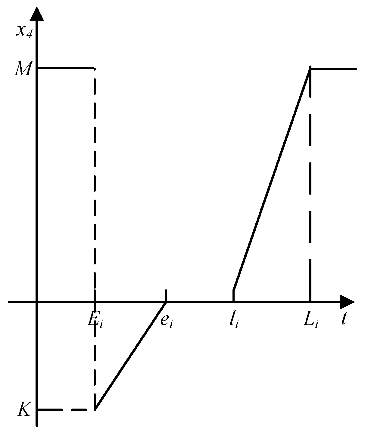
Incentive costs

The Incentive costs function is shown in Figure 2. If the vehicle arrives at customer $i$ in $\left(E_i,e_i\right)$, it will be rewarded for improving the freshness of the product. If the vehicle arrives within expectation time window $\left(e_i,l_i\right)$, no fees will be incurred. However, an additional penalty cost should be paid when the vehicle arrives in $\left(l_i,L_i\right)$. The incentive costs can be expressed in Equation (4).

$$x_4=\left\{\begin{array}{l}{P}_1\left(e_i-t_i^1\right),E_i<t_i^1<e_i\\ 0,e_i<t_i^1<l_i\\ P_2\left(t_i^1-l_i\right),l_i<t_i^1<L_i\\ \infty ,t_i^1<E_i\mathsf{\&}{t}_i^1<L_i\end{array}\right. \forall i\in V$$

(4)

3.3. Model Formulation

Based on the above analysis, the EVRP-MTCD-STW can be formulated as follows:

$$min\left(x_1+x_2+x_3+x_4\right)$$

(5)

Subject to:

$${\displaystyle \sum _{k\in K}{\displaystyle \sum _{i,j\in V}{x}_{ijk}}}=1$$

(6)

$$0\le w_{ij}\le Q i=0,\forall j\in V$$

(7)

$$t_j^1={\displaystyle \sum _{j\in V/\left\{0\right\};i\ne j}{x}_{ijk}\left(t_i^2+t_{ij}\right)} \forall i\in V,k\in K$$

(8)

$$P_{ck}^1=B \forall c\in C,k\in K$$

(9)

$$0\le P_{jk}^2\le P_{ik}^2-\xi d_{ij}{x}_{ijk}+B\left(1-x_{ijk}\right) \forall k\in K,\forall j\in V\cup C,\forall i\in V/\left\{0\right\},i\ne j$$

(10)

$$0\le P_{jk}^2\le B-\zeta d_{ij}{x}_{ijk} \forall k\in K,\forall j\in V\cup C,\forall i\in C\cup \left\{0\right\},i\ne j$$

(11)

$${\displaystyle \sum _{m\in M}{N}_m^k}\le h \forall k\in K$$

(12)

$${\displaystyle \sum _{i\in V}{\displaystyle \sum _{j\in V/\left\{0\right\}}{s}_{jm}}{x}_{ijk}\le L{N}_m^k} \forall k\in K,\forall m\in M$$

(13)

$$\frac{{\displaystyle \sum _{m\in M}{\displaystyle \sum _{i,j\in V}{z}_{jmk}{s}_{jm}\left(1-e^{-\delta t_{ijk}}\right)}}}{{\displaystyle \sum _{m\in M}{\displaystyle \sum _{j\in V}{S}_{jm}}}}\le F \forall k\in K$$

(14)

The objective function (5) optimizes the total distribution cost. Constraint (6) guarantees that each customer is served exactly once by one vehicle. Constraint (7) guarantees that the vehicle departs from the depot with a goods load not exceeding the maximum vehicle load. Constraint (8) defines the time to reach node $j$. Constraint (9) ensures that the vehicle leaves the charging station with a full charge. Constraint (10) and (11) represent the power consumption of the vehicle during transit. Specifically, when the vehicle reaches node $j$ subsequent to traversing node $i$, the residual power at node $j$ is determined by subtracting the power consumed from node $i$ to node $j$ from the residual power at node $i$. This calculation ensures that the remaining power at each node is sufficient to reach the next node, while simultaneously ensuring that the residual power at any given node throughout the transportation process does not exceed the vehicle battery capacity. In addition, the power relationship of the vehicle upon arrival at node j after departing from the charging station or depot in a fully charged state is also represented in constraint (11). Constraint (12) indicates that the number of insulation box loaded on each vehicle should not exceed the maximum number that the vehicle can accommodate. Constraint (13) ensures that the sum of the requirements for each vehicle loaded with goods of type m is less than the maximum capacity of insulation box. Constraint (14) ensures that the goods loss rate is within the acceptable range, at the moment the freshness of goods is: $F\left(t\right)=e^{-\delta t}$.

4. IACO Algorithm for EVRP-MTCD-STW

The traditional ACO has the problems of blind search, easy to fall into local optimum, and slow convergence speed. We introduce the conservation matrix, time window waiting factor, and frozen product impact factor to guide the ant search. We also improve the volatility factor to enhance the convergence speed, and embed the 2-opt algorithm to improve the local search ability.

4.1. Modification of State Transfer Rules

A suitable formulation of state transfer rules can improve the solving efficiency of the algorithm. To avoid repeated route selection during the search process, a selection strategy combining deterministic and random selection will be used, and dynamic adjustment transfer probability. Different from TSP, in VRP, multiple vehicles are delivered to different customers from the depot. As shown in Figure 3, to effectively save the number of delivery vehicles and mileage, a saving matrix is introduced to adjust the state transfer probability, which is shown in Equation (15).

$$u\left(i,j\right)=d\left(i,0\right)+d\left(0,j\right)-d\left(i,j\right)$$

(15)

In Equation (15), $u\left(i,j\right)$ denotes the distance saving from customer $i$ to customer $j$, $d\left(i,0\right)$ denotes the distance of the vehicle from customer $i$ to distribution center 0, $d\left(0,j\right)$ denotes the distance of the vehicle from distribution center 0 to customer $j$, $d\left(i,j\right)$ denotes the distance from customer $i$ to customer $j$.

To reduce the waiting time under the time window constraint, a time window waiting factor $wai{t}_j$ is introduced to prioritize the customers with a short waiting time. The time window waiting factor is shown in Equation (16).

$$wai{t}_j=\left\{\begin{array}{l}{e}_j-t_j,t_j<e_j\\ 1,e_j\le t_j\le l_j\\ t_j-l_j,t_j>l_j\end{array}\right.$$

(16)

where $t_j$ denotes the time of the vehicle arriving at customer $j$, $\left(e_j,l_j\right)$ denotes the expected time window for customer $j$. If $t_j<e_j$, the time window waiting factor $wai{t}_j=e_j-t_j$; If $e_j\le t_j\le l_j$, the time window waiting factor $wai{t}_j=1$; If $t_j>l_j$, the time window waiting factor $wai{t}_j=t_j-l_j$.

In cold chain logistics, temperature changes make the low-temperature goods more perishability. Therefore, the frozen product impact factor $col{d}_j$ is introduced in the state transfer probability. As shown in Equation (17), the customers with high demand for low-temperature goods are given priority in the following node selection.

$$col{d}_j=\frac{s_{j3}}{s_{j1}+s_{j2}+s_{j3}}$$

(17)

where $s_{jk}$ denotes the demand for different temperature zones, $k=1,2,3$ denotes the demand for normal temperature, refrigerated, and frozen goods.

The pheromone concentration determines the route selection probability. If it is too high, the solution will fall into a local optimum. Referring to the state transfer rule of the ant colony system [42], this paper introduces a constant $R$ to increase the search range by comparing the size with a random number $r\left(r\in \left[0,1\right]\right)$. The next node $j$ is determined as shown in Equation (18).

$$j=\left\{\begin{array}{l}\mathit{arg}\mathit{max}\left[{\tau }_{ij}^{\alpha }\left(t\right){\eta }_{ij}^{\beta }\left(t\right)u_{ij}col{d}_j\frac{1}{wai{t}_j}\right],r<R\\ p_{ij}^k\left(t\right),otherwise\end{array}\right.$$

(18)

where ${\tau }_{ij}\left(t\right)$ denotes the pheromone concentration on route $\left(i,j\right)$ at $t$. ${\eta }_{ij}\left(t\right)$ denotes the expectation degree of route $\left(i,j\right)$ at $t$, ${\eta }_{ij}\left(t\right)=1/d_{ij}$. $u_{ij}$ denotes the savings matrix of route $\left(i,j\right)$. $\alpha$ denotes the information heuristic factor. $\beta$ denotes the expectation heuristic factor.

The state transfer probability $p_{ij}^k\left(t\right)$ is shown in Equation (19).

$$p_{ij}^k\left(t\right)=\left\{\begin{array}{l}\frac{{\tau }_{ij}^{\alpha }\left(t\right){\eta }_{ij}^{\beta }\left(t\right)u_{ij}col{d}_j\frac{1}{wai{t}_j}}{{\displaystyle \sum _{j\in A_k}{\tau }_{ij}^{\alpha }\left(t\right){\eta }_{ij}^{\beta }\left(t\right)u_{ij}{s}_j\frac{1}{wai{t}_j}}},j\in A_k\\ 0,otherwise\end{array}\right.$$

(19)

where $A_k$ denotes the node that has not yet been distributed.

4.2. Improved Volatility Factor

The pheromone volatility factor $\rho$ refers to the pheromone disappearance level, and its value affect the algorithm’s convergence speed and global search ability. An appropriate setting of the pheromone volatility factor can improve the operation efficiency of the algorithm. Based on the existing research, we randomly select different values in different iteration ranges within a reasonable value range [0.2,0.5], as shown in Equation (20).

$$\rho =\left\{\begin{array}{l}0.2+rand/10,0\le n\le 0.25N\\ 0.3+rand/10,0.25N<n\le 0.75N\\ 0.4+rand/10,0.75N<n\le N\end{array}\right.$$

(20)

where rand denotes the random number between $\left(0,1\right)$, which follows a uniform random distribution. $n$ denotes the current number of iterations. $N$ denotes the maximum number of iterations.

In the early iteration, the value of $\rho$ is set to a smaller number to expand the ant search range and find a better value in the global search. In the middle iteration, the route has accumulated more pheromones, so the value of $\rho$ is increased to prevent the algorithm from converging quickly and falling into the local optimum. In the late iteration, the value of $\rho$ is continuously increased to find the optimal solution to accelerate the convergence speed.

4.3. Local Search Optimization

As a local search optimization algorithm, the core of the 2-opt algorithm is to randomly select an interval segment for optimization. Although optimization only optimizes the current state, we can improve the convergence speed of ACO by introducing the 2-opt algorithm and effectively solve the problem of the algorithm quickly falling into local optima. It improves the efficiency of local search without affecting the overall performance of the ACO algorithm.

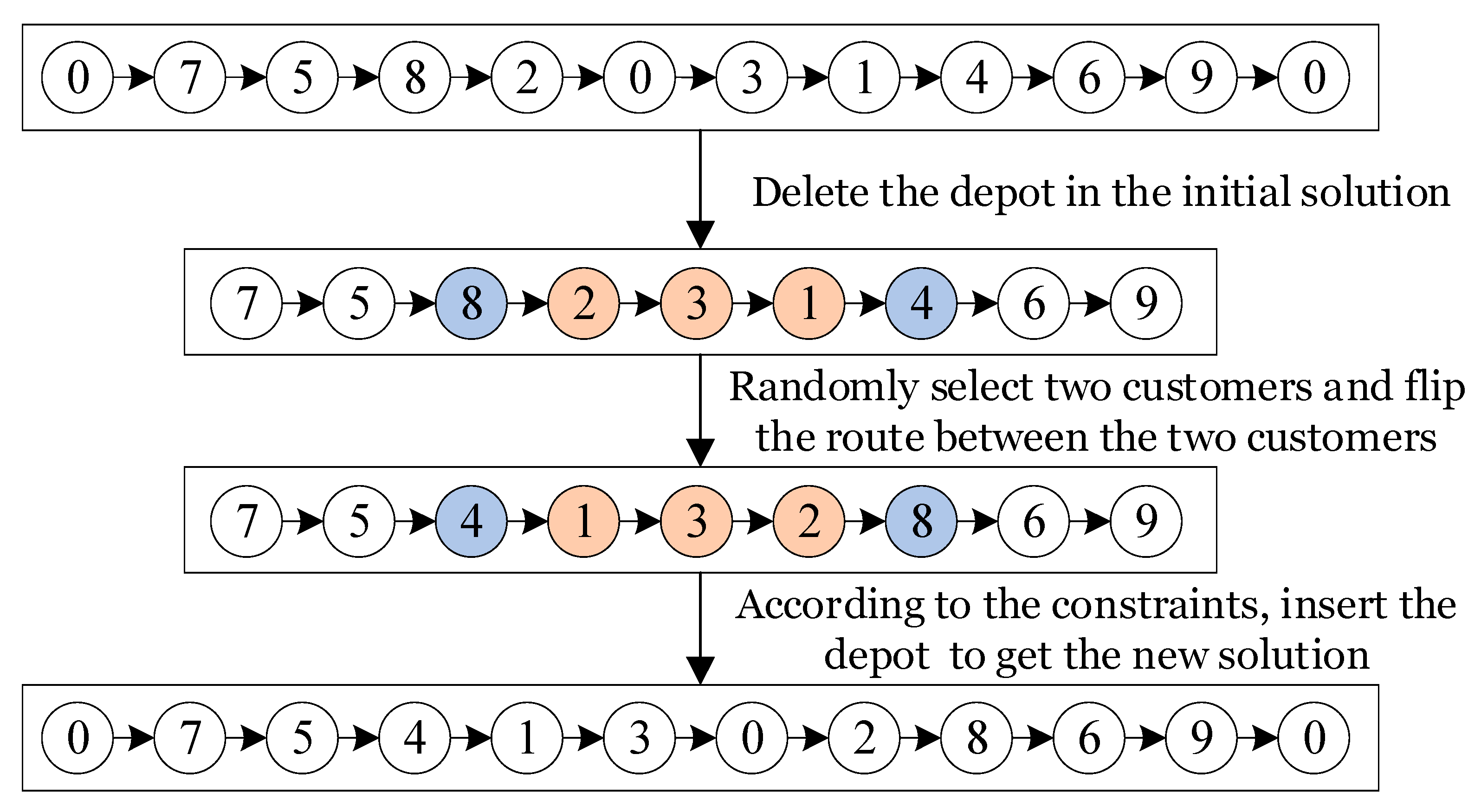
In the VRP, the basic principle of the 2-opt method is to delete the depot node in the optimal solution obtained by the current iteration, randomly select two customers and flip the route between the two customers, keep the order of other customers unchanged. Next based on constraints, insert the depot to get the new route. Then judge whether the solution of the new route is better than the initial solution, if it is better, replace the initial solution, and if not, keep the initial solution and continue the iteration. The specific process is shown in Figure 4.

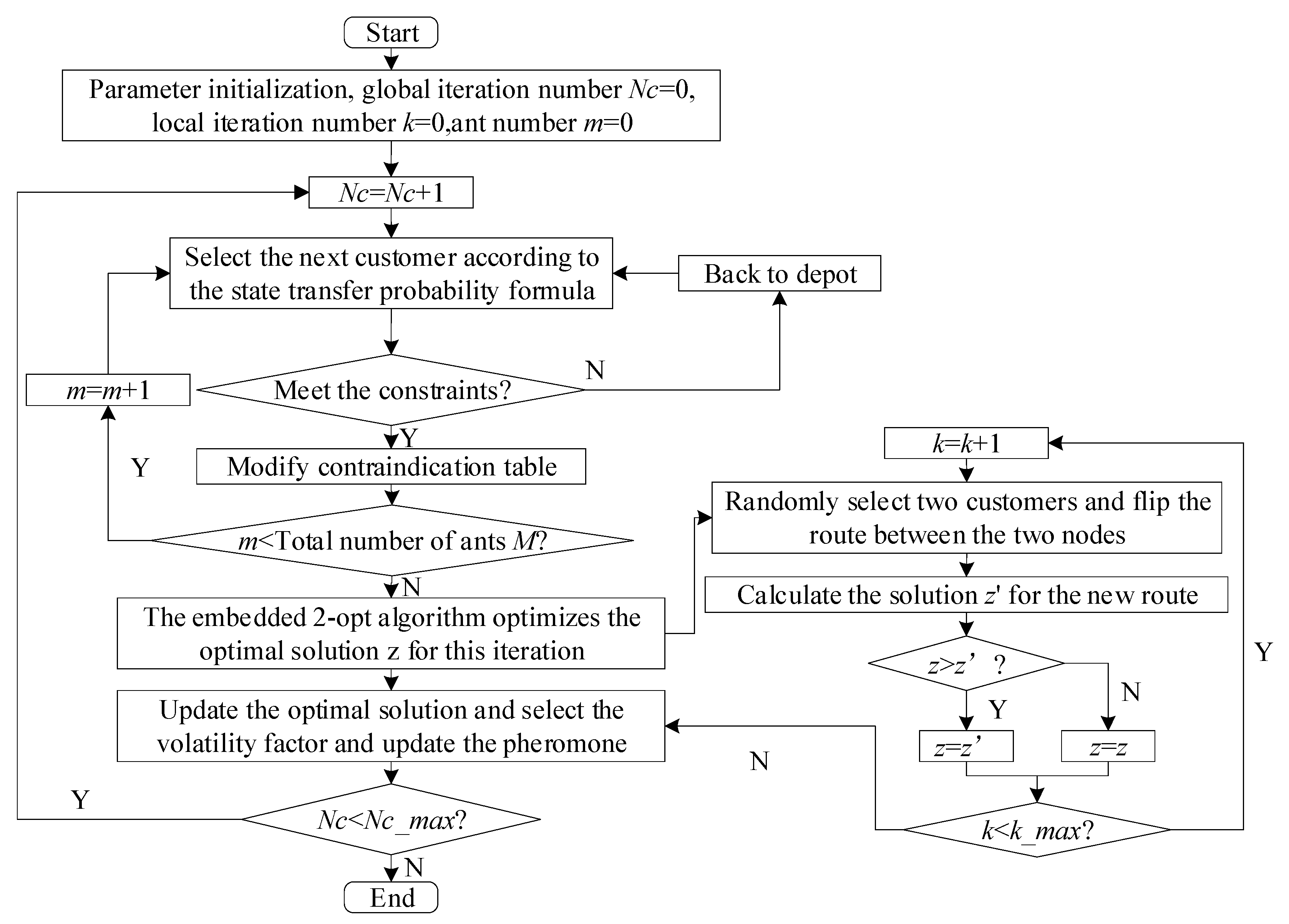
4.4. The Main Steps of IACO

Based on the procedures presented in Section 4.1, Section 4.2 and Section 4.3, the main steps of the IACO for solving EVRP-MTCD-STW are shown as follows.

Step 1. Initialization of parameters, including a maximum number of iterations, ant colony size, information heuristic factor, expectation heuristic factor, etc.

Step 2. Place all ants at the distribution centroid and create a contraindication table to record ant walking routes.

Step 3. Determine the next customer selected by the ant according to Equations (15)–(19).

Step 4. Determine whether the constraint is satisfied. If so, continue to find the next customer; otherwise return to the depot.

Step 5. Repeat steps 3 and 4 until all customers are served, and update ant count.

Step 6. Embed the 2-opt algorithm to adjust the optimal route of this iteration after all ants have completed customer service.

Step 7. After updating the optimal solution, the pheromone is updated by selecting the volatility factor according to Equation (20).

Step 8. Determine if the maximum number of iterations is reached. If not, add 1 to the number of iterations and return to step 2; otherwise, end the program and output the optimal value.

The whole process is shown in Figure 5.

5. Computational Experiments

In this section, we first evaluate the performance of IACO by comparing with other literatures based on Solomon dataset. Next, we create EVRP-MTCD-STW instances, and solve it with IACO. Then, we analyze the distribution mode and the change of time window width. The experiments were run using MATLAB R2017b software on a PC with an i5-6200U processor, 4G RAM, and Windows 10 64-bit operating system.

5.1. Parameter Setting

Based on the relevant parameters provided in the literature [43,44], we conduct repeated experiments and obtained the algorithm and model parameters as shown in

Table 2. Algorithm and model parameter settings.

Parameter	Description	Value
Algorithm
$m$	Ant number	100
$\alpha$	Pheromone importance	1
$\beta$	Heuristic factor importance	5
$\rho$	Initial pheromone volatility factor	0.2
$Nc\_\mathit{max}$	Iteration number	200
Model
$P_1$	Reward coefficient	−0.5
$P_2$	Penalty coefficient	1
$f_1$	Cost of using normal temperature vehicle (CNY)	500
$f_2$	Cost of using refrigerated vehicle (CNY)	550
$f_3$	Cost of using frozen vehicle (CNY)	575
$e$	Vehicle unit transportation cost (CNY/km)	2
$g$	Insulation box cost (CNY)	0.5
$g_2$	Refrigerated cooler cost (CNY)	1
$g_3$	Frozen cooler cost (CNY)	1.6
$\omega$	Vehicle charging cost (CNY/kWh)	0.747
$B$	Vehicle battery capacity (kWh)	80
$\xi$	Unit mileage power consumption (kWh/km)	0.055
$Q$	Maximum load of the vehicle (kg)	200
$h$	Number of insulation box that can be accommodated per vehicle	15
$L$	Maximum capacity of insulation box (kg)	12
$\delta$	Loss rate of goods	0.03
$F$	Maximum acceptable goods loss rate	20%

.

5.2. Efficiency Assessment of IACO

The benchmark test instances for EVRP-MTCD-STW are currently unavailable. As EVRP-MTCD-STW is an extension of VRPTW, we validate the effectiveness of the proposed IACO using the Solomon dataset, which is an internationally recognized standard test set widely used for VRPTW. The Solomon dataset contains 56 instances covering six different problem types: C1, C2, R1, R2, RC1, and RC2. Where type refers to:

C: the locations of customers are geographically clustered;

R: the locations of customers are randomly distributed;

RC: the locations of customers are a mixture of clustering and random distribution;

Type1: the customer’s time window is narrow and the vehicle capacity is small;

Type2: the customer’s time window is wide and the vehicle capacity is large.

IACO is used to test 12 instances with a customer scale of 100, including C1, C2, R1, R2, RC1, and RC2 types. Each instance is tested 10 times. The experimental analysis is conducted with the objective of minimizing the distance travelled under conditions that allowed for time window relaxation. Set soft time window $E_i=e_i-0.5\left(l_i-e_i\right)$, $L_i=l_i+0.5\left(l_i-e_i\right)$.

The optimal solutions of IACO algorithm are compared with the best-known solutions (BSK), the two-phase tabu search algorithm (TP-TS), and the simulated annealing heuristic with restart strategy (SARS) [45,46], as shown in

Table 3. Comparison of IACO algorithm with other algorithms for optimal solutions.

Dataset	BKS		TP-TS		SARS		IACO		∆x%
	NV	TD	NV	TD	NV	TD	NV	TD
C101	10	828.94	10	829.01	10	828.94	10	828.94	0
C102	10	828.94	10	832.56	10	828.94	10	828.94	0
C201	3	591.56	3	591.58	3	591.56	3	591.56	0
C202	3	591.56	3	591.58	3	591.56	3	591.56	0
R101	19	1645.79	20	1653.54	20	1644.26	16	1425.82	−13.29
R102	17	1486.12	19	1488.00	19	1481.9	15	1367.56	−7.72
R201	4	1252.37	5	1216.33	9	1167.53	7	1098.56	−5.91
R202	3	1191.70	4	1131.75	9	1053.5	7	1019.24	−3.25
RC101	14	1696.94	16	1653.06	17	1664.06	14	1513.66	−8.43
RC102	12	1554.75	14	1502.16	15	1489.22	12	1336.57	−10.25
RC201	4	1406.91	4	1470.12	9	1287.05	8	1232.67	−4.23
RC202	3	1367.09	4	1208.10	9	1109.51	7	1099.10	−0.94

. In this table, Column 1 report the name of dataset. Columns 2–9 respectively report the number of vehicles (NV) and total distance (TD) used in the optimal solution obtained using BKS, TP-TS, SARA and IACO. Column 10 reports the difference between the distance of the optimal solution obtained by IACO and the optimal distance obtained by the comparative algorithm, $\Delta x=\left(T{D}_{IACO}-T{D}_{best\_other}\right)/T{D}_{best\_other}\times 100\%$.

According to the results in Table 3, IACO proposed in this study can find the optimal solution for both the number of vehicles used and the distance travelled in all four datasets of type C. In other datasets, the distance is improved to varying degrees. It is worth noting that due to the narrower time window of datasets R101 and RC101 compared to datasets R201 and RC201, the difference in optimal distance is greater, exceeding 7%. In datasets R2 and RC2, although the number of vehicles is used more than the number in BKS, both are less than the number of vehicles found by the SARS algorithm. The above comparative analysis shows that the IACO proposed in this paper is feasible for solving the VRPTW.

5.3. Computational Results for EVRP-MTCD-STW Instance

For the consideration of the timeliness of cold chain goods and the mileage of EVs, we selected some nodes from dataset R101 to construct an EVPRP-MTCD-STW instance. The demand data for each customer’s product in different temperature zones is obtained using the unbalanced partitioning strategy proposed by Fallahi et al. [47]. Moreover, the charging station locations are randomly selected with the method proposed by Schneider et al. [24].

Table 4. The adapted dataset R101 for EVRP-MTCD-STW.

No.	X (km)	Y (km)	Demand (kg)	D1 (kg)	D2 (kg)	D3 (kg)	T1 (min)	T2 (min)
0	35	35	0	0	0	0	0	230
1	5	5	25	5	13	7	167	187
2	4	18	16	4	4	8	36	56
3	10	43	20	6	10	4	90	110
4	15	10	19	5	8	6	148	168
5	6	68	26	5	12	9	29	49
6	2	60	24	12	3	9	89	109
7	27	69	13	3	7	3	46	66
8	20	50	9	2	3	4	146	66
9	30	60	25	8	9	8	119	139
10	41	49	34	8	12	14	93	103
11	49	73	18	8	3	7	62	82
12	40	60	35	8	9	18	66	86
13	62	77	23	7	6	10	156	176
14	57	48	28	10	10	8	27	47
15	65	35	19	6	5	8	78	98
16	67	5	30	9	9	12	177	197
17	53	12	26	7	9	10	163	183
18	45	10	33	13	8	12	125	145
19	32	12	17	4	6	7	96	116
20	22	27	38	7	16	15	29	49
21	50	35	30	8	13	9	58	78
22	65	20	36	9	12	15	87	107
23	23	3	29	9	7	13	127	147
24	49	58	28	12	5	11	103	123
25	15	30	32	9	15	8	130	150
26	50	20	0	0	0	0	0	230
27	16	56	0	0	0	0	0	230
28	35	12	0	0	0	0	0	230
29	15	35	0	0	0	0	0	230
30	40	55	0	0	0	0	0	230

shows data from the adapted dataset R101 for EVRP-MTCD-STW. Column 1 reports set number, number 0 is the depot, 1 to 25 are customers, and 26 to 30 are charging stations. Columns 2,3 report coordinate information of points. Columns 4–7 report total demand, demand for normal temperature goods, demand for refrigerated goods and demand for frozen goods respectively. Columns 8,9, respectively, report expectation left time window and right time window. The Euclidean distance, based on their positional coordinates, is used to calculate the distance between nodes.

(1)

Results of solving adapted dataset R101

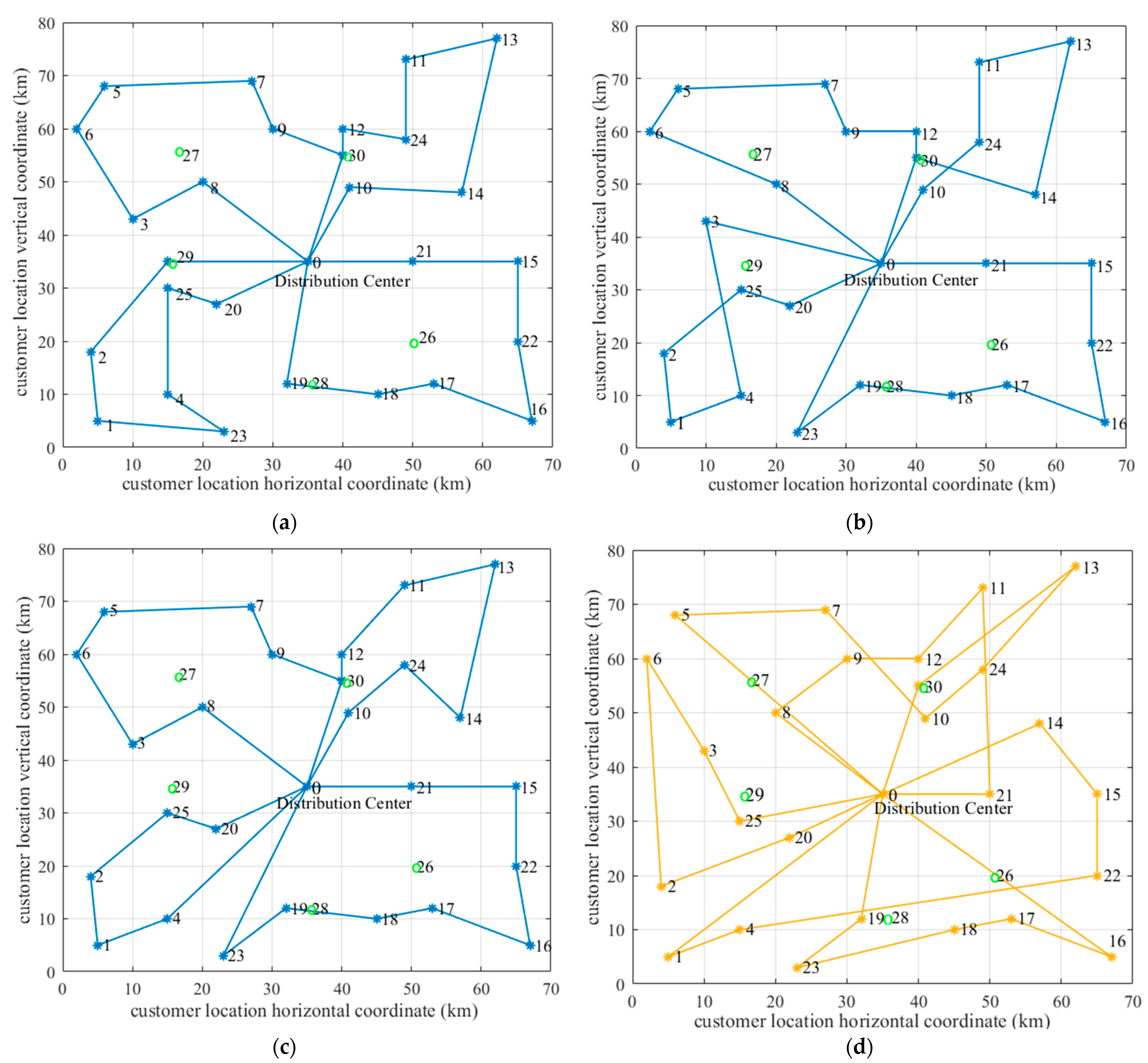
Through several experiments, the results were obtained, as shown in the graphs.

Table 5. Vehicle distribution route.

Vehicle	Route
Vehicle 1	0-5-7-10-24-13-30-0
Vehicle 2	0-20-2-6-3-25-0
Vehicle 3	0-14-15-22-4-1-0
Vehicle 4	0-21-11-12-9-8-0
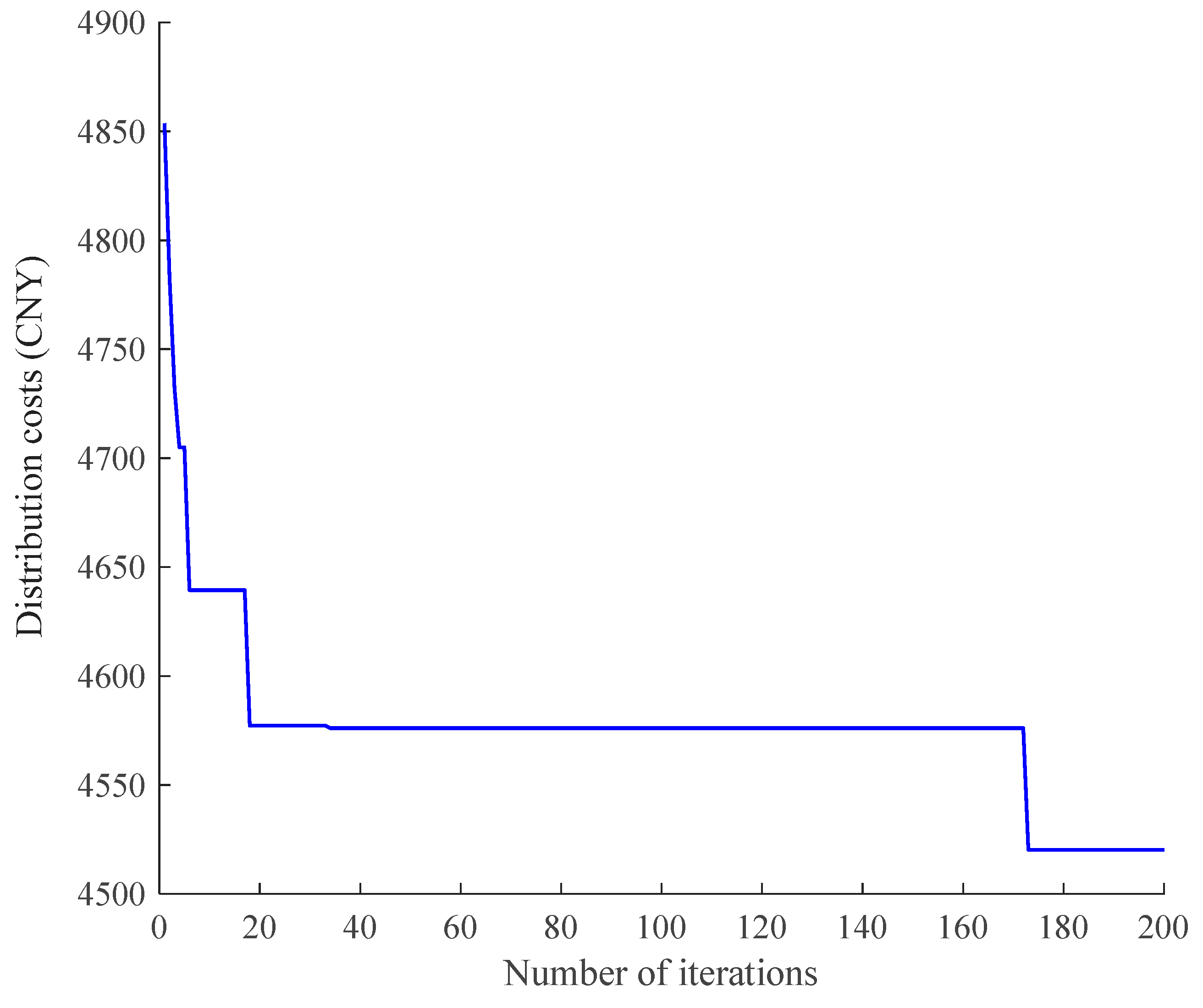
Vehicle 5	0-19-23-18-17-16-0

shows the vehicle distribution route when the value of the distribution cost is optimal, Figure 6 shows the iterative convergence, and Figure 7d shows the vehicle distribution route. The optimal distribution cost is CNY 4520.20; the optimal solution is obtained at the 173rd iteration, using five EVs and passing through the charging station once.

(2)

Influence of distribution mode

The analysis compares the results of single temperature distribution (STD) and MTCD based on the primary example. Carrying out STD vehicles can only transport single-temperature products, and different vehicles are needed to distribute products in different temperature zones at each customer.

Figure 7 compares vehicle distribution routes for STD and MTCD with 25 customers. We can see that four vehicles are needed for the distribution of goods in one temperature zone for STD. During the distribution period, the normal temperature goods need to go to the charging station twice, and the refrigerated and frozen goods need to go to the charging station once. If goods in three temperature zones are distributed separately, 12 vehicles are needed, and the charging station needs to be visited four times. If the MTCD is carried out, five vehicles are needed for distribution. Only one visit to the charging station is required to replenish the power during the distribution period. Therefore, MTCD can save resources and has specific efficiency.

Table 6. Cost comparison between STD and MTCD models.

Method	Cost (CNY)	Transportation (CNY)	Refrigeration (CNY)	Charging (CNY)	Incentive (CNY)
Single	8941.16	8340.18	480	93.46	27.52
Multi	4520.2	3941.12	572.9	41.39	−35.21

shows the cost comparison between a STD and a MTCD. The refrigeration cost of MTCD is 19.35% more than that of STD, however, the total cost of the MTCD is 49.45% lower than that of the STD. Due to more vehicles used in STD, leading to higher transportation costs. Therefore, the use of MTCD will be more resource saving and efficient. The relevant logistics enterprises can reasonably choose the distribution mode according to customer demand.

(3)

Influence of the width of the time window

The results of 50%, 100%, 150%, and 200% expansion of the customers’ desired time window were compared to investigate the effect of soft time window changes on the distribution results. As shown in

Table 7. Comparative analysis of the change of time window width.

Expands	Cost (CNY)	Incentive (CNY)	Vehicle
0%	6234.21	28.48	8
50%	5120.73	6.8	6
100%	4520.20	−35.21	5
150%	4460.52	−52.52	5
200%	4432.88	−61.09	5

, the number of vehicles required decreases as the time window width gradually expands, the total cost of distribution also decreases. The number of vehicles reaches the lowest when the time window width expands to 100%.

The probability of vehicles arriving at the customer earlier increases with the widening of the time window. As a result, the cost of rewards increases, the cost of punishment decreases, and the cost of incentives increases in the opposite direction. Therefore, when the customers’ time window requirements are relatively low, appropriately expanding the time window width will deliver goods as early as possible, improve delivery efficiency and reduce distribution cost.

6. Conclusions and Future Research

In this paper, we introduce a variant of the EVs routing problem, considering multi-temperature co-distribution and soft time windows. Each EVs can deliver three kinds of temperature goods, and the temperature is controlled by a cooler. Considering the power, time windows, load, and cargo loss rate constraints, a mathematical model of EVRP-MTCD-STW with the objective of minimizing the distribution costs is established.

In addition, to effectively solve EVRP-MTCD-STW, we propose the IACO algorithm, which introduces the distance saving matrix, time window waiting factor, and frozen product influence factor to modify the state transfer rules, and insert the 2-opt algorithm to improve the optimization capability. Finally, we verify the validity of the algorithm and analyze the model based on the Solomon dataset. The numerical experiments demonstrate that the IACO proposed in this paper can find high-quality solutions compared to other algorithms in the literature. Utilizing EVs for multi-temperature co-distribution can improve distribution efficiency of cold chain logistics and provide innovative ideas for development of logistics companies, and setting appropriate soft time windows can ensure freshness of goods while reducing distribution costs.

Several directions for future research can be considered. One is to include more realistic constraints in the mathematical model, such as the uncertainty of travel time caused by weather changes and road accidents, or the dynamic changes in customer demand, to meet the challenges of real-world distribution. Second, the energy consumption of EVs is not only related to the distance travelled, but also affected by many factors such as load, road conditions, ambient humidity, etc., so another topic for future research is how to incorporate these factors to accurately represent the energy consumption of EVs in the distribution process. Finally, more effective local optimization strategies can be designed to improve the performance of the algorithm in solving large-scale problems.

References

- Li, Z.; Khajepour, A.; Song, J. A comprehensive review of the key technologies for pure electric vehicles. Energy 2019, 182, 824–839. [Google Scholar] [CrossRef]
- Chen, D.; Ignatius, J.; Sun, D.; Goh, M.; Zhan, S. Impact of congestion pricing schemes on emissions and temporal shift of freight transport. Transp. Res. Part E Logist. Transp. Rev. 2018, 118, 77–105. [Google Scholar] [CrossRef]
- Liu, W.; Wang, M.; Zhu, D.; Zhou, L. Service capacity procurement of logistics service supply chain with demand updating and loss-averse preference. Appl. Math. Model. 2019, 66, 486–507. [Google Scholar] [CrossRef]
- Luo, H.; Dridi, M.; Grunder, O. A branch-and-price algorithm for a routing and scheduling problem from economic and environmental perspectives. RAIRO-Oper. Res. 2022, 56, 3267–3292. [Google Scholar] [CrossRef]
- Liu, G.; Hu, J.; Yang, Y.; Xia, S.; Lim, M.K. Vehicle routing problem in cold Chain logistics: A joint distribution model with carbon trading mechanisms. Resour. Conserv. Recy. 2020, 156, 104715. [Google Scholar] [CrossRef]
- Yan, L.; Grifoll, M.; Zheng, P. Model and Algorithm of Two-Stage Distribution Location Routing with Hard Time Window for City Cold-Chain Logistics. Appl. Sci. 2020, 10, 2564. [Google Scholar] [CrossRef]
- Gao, J.; Zhen, L.; Wang, S. Multi-trucks-and-drones cooperative pickup and delivery problem. Transp. Res. Part C Emerg. Technol. 2023, 157, 104407. [Google Scholar] [CrossRef]
- Lian, J. An optimization model of cross-docking scheduling of cold chain logistics based on fuzzy time window. J. Intell. Fuzzy Syst. 2021, 41, 1901–1915. [Google Scholar] [CrossRef]
- Dantzig, G.B.; Ramser, J.H. The Truck Dispatching Problem. Manag. Sci. 1959, 6, 80–91. [Google Scholar] [CrossRef]
- Abdulkader, M.M.S.; Gajpal, Y.; ElMekkawy, T.Y. Hybridized ant colony algorithm for the Multi Compartment Vehicle Routing Problem. Appl. Soft Comput. 2015, 37, 196–203. [Google Scholar] [CrossRef]
- Molina, J.C.; Salmeron, J.L.; Eguia, I. An ACS-based memetic algorithm for the heterogeneous vehicle routing problem with time windows. Expert Syst. Appl. 2020, 157, 113379. [Google Scholar] [CrossRef]
- Halassi Bacar, A.; Rawhoudine, S.C. An attractors-based particle swarm optimization for multiobjective capacitated vehicle routing problem. RAIRO-Oper. Res. 2021, 55, 2599–2614. [Google Scholar] [CrossRef]
- Solomon, M.M. Algorithms for the Vehicle Routing and Scheduling Problems with Time Window Constraints. Oper. Res. 1987, 35, 254–265. [Google Scholar] [CrossRef]
- Hashimoto, H.; Yagiura, M.; Imahori, S.; Ibaraki, T. Recent progress of local search in handling the time window constraints of the vehicle routing problem. Ann. Oper. Res. 2013, 204, 171–187. [Google Scholar] [CrossRef]
- Xu, Z.; Elomri, A.; Pokharel, S.; Mutlu, F. A model for capacitated green vehicle routing problem with the time-varying vehicle speed and soft time windows. Comput. Ind. Eng. 2019, 137, 106011. [Google Scholar] [CrossRef]
- Lespay, H.; Suchan, K. Territory Design for the Multi-Period Vehicle Routing Problem with Time Windows. Comput. Oper. Res. 2022, 145, 105866. [Google Scholar] [CrossRef]
- Kang, H.; Lee, A. An Enhanced Approach for the Multiple Vehicle Routing Problem with Heterogeneous Vehicles and a Soft Time Window. Symmetry 2018, 10, 650. [Google Scholar] [CrossRef]
- Jie, K.; Liu, S.; Sun, X. A hybrid algorithm for time-dependent vehicle routing problem with soft time windows and stochastic factors. Eng. Appl. Artif. Intel. 2022, 109, 104606. [Google Scholar] [CrossRef]
- Ge, J.; Liu, X.; Guo, L. Research on Vehicle Routing Problem with Soft Time Windows Based on Hybrid Tabu Search and Scatter Search Algorithm. Comput. Mater. Contin. 2020, 64, 1945–1958. [Google Scholar] [CrossRef]
- Hu, L.; Xiang, C.; Qi, C.; Rajesh, K.; Kaluri, R. Optimization of VRR for Cold Chain with Minimum Loss Based on Actual Traffic Conditions. Wirel. Commun. Mob. Comput. 2021, 2021, 1–10. [Google Scholar] [CrossRef]
- Nolz, P.C.; Absi, N.; Feillet, D.; Seragiotto, C. The consistent electric-Vehicle routing problem with backhauls and charging management. Eur. J. Oper. Res. 2022, 302, 700–716. [Google Scholar] [CrossRef]
- Keskin, M.; Çatay, B. Partial recharge strategies for the electric vehicle routing problem with time windows. Transp. Res. Part C Emerg. Technol. 2016, 65, 111–127. [Google Scholar] [CrossRef]
- Seyfi, M.; Alinaghian, M.; Ghorbani, E.; Çatay, B.; Saeid Sabbagh, M. Multi-mode hybrid electric vehicle routing problem. Transp. Res. Part E Logist. Transp. Rev. 2022, 166, 102882. [Google Scholar] [CrossRef]
- Schneider, M.; Stenger, A.; Goeke, D. The Electric Vehicle-Routing Problem with Time Windows and Recharging Stations. Transp. Sci. 2014, 48, 500–520. [Google Scholar] [CrossRef]
- Macrina, G.; Di Puglia Pugliese, L.; Guerriero, F.; Laporte, G. The green mixed fleet vehicle routing problem with partial battery recharging and time windows. Comput. Oper. Res. 2019, 101, 183–199. [Google Scholar] [CrossRef]
- Hiermann, G.; Puchinger, J.; Ropke, S.; Hartl, R.F. The Electric Fleet Size and Mix Vehicle Routing Problem with Time Windows and Recharging Stations. Eur. J. Oper. Res. 2016, 252, 995–1018. [Google Scholar] [CrossRef]
- Desaulniers, G.; Errico, F.; Irnich, S.; Schneider, M. Exact Algorithms for Electric Vehicle-Routing Problems with Time Windows. Oper. Res. 2016, 64, 1388–1405. [Google Scholar] [CrossRef]
- Goeke, D.; Schneider, M. Routing a mixed fleet of electric and conventional vehicles. Eur. J. Oper. Res. 2015, 245, 81–99. [Google Scholar] [CrossRef]
- Hsu, C.; Chen, W. Optimizing fleet size and delivery scheduling for multi-temperature food distribution. Appl. Math. Model. 2014, 38, 1077–1091. [Google Scholar] [CrossRef]
- Kuo, J.; Chen, M. Developing an advanced Multi-Temperature Joint Distribution System for the food cold chain. Food Control 2010, 21, 559–566. [Google Scholar] [CrossRef]
- Ostermeier, M.; Hübner, A. Vehicle selection for a multi-compartment vehicle routing problem. Eur. J. Oper. Res. 2018, 269, 682–694. [Google Scholar] [CrossRef]
- Oppen, J.; Løkketangen, A. A tabu search approach for the livestock collection problem. Comput. Oper. Res. 2008, 35, 3213–3229. [Google Scholar] [CrossRef]
- Li, Y.M.; Chen, Y.A. Assessing the thermal performance of three cold energy storage materials with low eutectic temperature for food cold chain. Energy 2016, 115, 238–256. [Google Scholar] [CrossRef]
- Chen, W.; Hsu, C. Greenhouse gas emission estimation for temperature-controlled food distribution systems. J. Clean. Prod. 2015, 104, 139–147. [Google Scholar] [CrossRef]
- Bai, Q.; Yin, X.; Lim, M.K.; Dong, C. Low-carbon VRP for cold chain logistics considering real-time traffic conditions in the road network. Ind. Manag. Data Syst. 2022, 122, 521–543. [Google Scholar] [CrossRef]
- Oztas, T.; Tus, A. A hybrid metaheuristic algorithm based on iterated local search for vehicle routing problem with simultaneous pickup and delivery. Expert Syst. Appl. 2022, 202, 117401. [Google Scholar] [CrossRef]
- Li, N.; Li, G. Hybrid partheno-genetic algorithm for multi-depot perishable food delivery problem with mixed time windows. Ann. Oper. Res. 2022. [Google Scholar] [CrossRef]
- Colorni, A.; Dorigo, M.; Maffioli, F.; Maniezzo, V.; Righini, G.; Trubian, M. Heuristics from Nature for Hard Combinatorial Optimization Problems. Int. Trans. Oper. Res. 1996, 3, 1–21. [Google Scholar] [CrossRef]
- Kyriakakis, N.A.; Marinaki, M.; Marinakis, Y. A hybrid ant colony optimization-variable neighborhood descent approach for the cumulative capacitated vehicle routing problem. Comput. Oper. Res. 2021, 134, 105397. [Google Scholar] [CrossRef]
- Yu, B.; Yang, Z.Z. An ant colony optimization model: The period vehicle routing problem with time windows. Transp. Res. Part E Logist. Transp. Rev. 2011, 47, 166–181. [Google Scholar] [CrossRef]
- Jia, Y.; Mei, Y.; Zhang, M. Confidence-based Ant Colony Optimization for Capacitated Electric Vehicle Routing Problem with Comparison of Different Encoding Schemes. IEEE Trans. Evol. Comput. 2022, 26, 1394–1408. [Google Scholar] [CrossRef]
- Mutar, M.; Burhanuddin, M.; Hameed, A.; Yusof, N.; Mutashar, H. An efficient improvement of ant colony system algorithm for handling capacity vehicle routing problem. Int. J. Ind. Eng. Comput. 2020, 11, 549–564. [Google Scholar] [CrossRef]
- Murakami, K. A new model and approach to electric and diesel-powered vehicle routing. Transp. Res. Part E Logist. Transp. Rev. 2017, 107, 23–37. [Google Scholar] [CrossRef]
- Zhang, L.; Tseng, M.; Wang, C.; Xiao, C.; Fei, T. Low-carbon cold chain logistics using ribonucleic acid-ant colony optimization algorithm. J. Clean. Prod. 2019, 233, 169–180. [Google Scholar] [CrossRef]
- Jiang, J.; Ng, K.M.; Poh, K.L.; Teo, K.M. Vehicle routing problem with a heterogeneous fleet and time windows. Expert Syst. Appl. 2014, 41, 3748–3760. [Google Scholar] [CrossRef]
- Yu, V.F.; Winarno; Maulidin, A.; Redi, A.A.N.P.; Lin, S.; Yang, C. Simulated Annealing with Restart Strategy for the Path Cover Problem with Time Windows. Mathematics 2021, 9, 1625. [Google Scholar] [CrossRef]
- Fallahi, A.E.; Prins, C.; Wolfler Calvo, R. A memetic algorithm and a tabu search for the multi-compartment vehicle routing problem. Comput. Oper. Res. 2008, 35, 1725–1741. [Google Scholar] [CrossRef]