Article

Position Estimation Method for Unmanned Tracked Vehicles Based on a Steering Dynamics Model

1
Army Academy of Armored Forces, Beijing 100072, China
2
Unit 63963 of PLA, Beijing 100072, China
*
Author to whom correspondence should be addressed.
World Electr. Veh. J. 2024, 15(3), 120; https://doi.org/10.3390/wevj15030120
Submission received: 29 February 2024 / Revised: 15 March 2024 / Accepted: 16 March 2024 / Published: 21 March 2024

Abstract

:
A position estimation method for unmanned tracked vehicles based on a steering dynamics model was developed during this study. This method can be used to estimate the position of a tracked vehicle in real time without relying on a high-precision positioning system. First, the relationship between the shear displacement of the track relative to the ground and the speed and yaw rate of the tracked vehicle during the steering process was analyzed. Next, the steering force of the tracked vehicle was calculated by using the shear force–displacement theory, and a steering dynamics model considering the acceleration of the vehicle was established. The experimental results show that this steering dynamics model produced more accurate position estimations for an unmanned tracked vehicle than did the kinematics model. This method can serve as a reference for the positioning of unmanned tracked vehicles working in special environments that cannot use precise positioning systems.

1. Introduction

Unmanned tracked vehicles have broad development prospects in the agriculture [1] and fire protection [2] fields due to their good trafficability and mobility characteristics. Real-time and accurate positioning is important for ensuring the normal operation of unmanned tracked vehicles. Currently, most of the accurate position information obtained for unmanned tracked vehicles is dependent on high-precision positioning systems, such as inertial navigation components and differential positioning devices [3,4]. For unmanned tracked vehicles working in special environments, such as woodland, mountain, or underground environments, the reliability of high-precision positioning systems is difficult to guarantee. Some unmanned tracked vehicles use the positioning method of matching radar point cloud and point cloud map. This method reduces the dependence of unmanned tracked vehicles on their high-precision positioning systems to a certain extent when they already have point cloud maps [5,6,7]. For unmanned tracked vehicles working in unknown or open environments, it is difficult to obtain the required positioning accuracy when using the point cloud matching method. Therefore, improving the positioning accuracy in special working environments without relying on high-precision positioning systems is very important to the further development of unmanned tracked vehicles.
Many scholars around the world have conducted research regarding position estimation methods for unmanned tracked vehicles that do not rely on high-precision positioning systems. The most traditional of these methods involves using the speed data of the active wheel of an unmanned tracked vehicle to estimate the real-time position of the vehicle from the steering kinematics model [8]. Because the kinematics model ignores the relative sliding between the tracks and the ground, this method produces large positioning errors [9]. Martinez [10] established an equivalent-steering approximate kinematics model, processed the original trajectory data of a vehicle using the genetic algorithm, and estimated the vehicle position in real time using a reliable positioning system. Xiong [11] established a vehicle kinematics model that considered the sliding parameters. During a vehicle turning process, by comparing the position estimated by the kinematics model with the position measured by a high-precision positioning system, the Leven–Marquardt algorithm was used to estimate the real-time sliding parameters. Rogers [12] established a three-dimensional kinematics model of a vehicle and used the Kalman filter algorithm to estimate the sliding parameters in real time using a high-precision positioning sensor. Moosavian [13] carried out a large number of real vehicle experiments. The sliding parameters in the experimental data were linearly fitted with the corresponding steering radius, and the vehicle position was corrected in real time by feedforward compensation. Using a kinematics model to estimate the position of an unmanned tracked vehicle reduces the dependence on a high-precision positioning system to some extent. However, to improve the position estimation accuracy, it is still necessary to correct the results obtained from the kinematics model in real time [14]. This paper proposes a position estimation method for unmanned tracked vehicles that is based on a steering dynamics model and then compares the results with those of a position estimation method based on a kinematics model.
Research regarding the steering force model for tracked vehicles is becoming increasingly mature. Purdy [15] used Coulomb’s law to calculate the steering force of tracked vehicles under the assumption that the ground pressure generated by the tracked vehicle is uniform. However, when a tracked vehicle turns while traveling at a high speed, the track force calculated by this model does not change as the steering radius changes. Thus, the calculated force does not conform to the actual track force during the turning process [16]. Under the assumption that the track is subjected to uniform force, Wong [17] analyzed the steady-state steering of tracked vehicles by using the shear force–displacement model. Tang [18] assumed that the tracked ground pressure was trapezoidal distribution when the tracked vehicle turned, and based on this assumption, the steady-state steering process of the tracked vehicle was analyzed. Under the assumption that the ground pressure of the track is rectangular and concentrated in each load wheel, Wang [19] calculated the relationship between the force of the track on both sides and the shear displacement under the steady steering condition of the tracked vehicle by using the numerical iteration method. For the study of steady-state steering of tracked vehicles, only the motion parameters in the steering process of tracked vehicles can be analyzed. It is necessary to study the dynamic steering process of tracked vehicles for position estimation and motion control of tracked vehicles. Özdemir [20] improved the steering dynamics model established by Wong and realized the analysis of the dynamic steering process of tracked vehicles.
During this study, the relationship between shear displacement and the speed and yaw rate during the steering process of tracked vehicles was systematically analyzed. The shear force–displacement model was used to calculate the track force, and a steering dynamics model suitable for real-time positioning of tracked vehicles was established. The proposed position estimation method for unmanned tracked vehicles was verified by simulations and experiments with actual vehicles. The experimental results showed that the position estimation method proposed in this paper, which does not rely on a high-precision positioning system, exhibited a better position estimation accuracy than a position estimation method based on the kinematics model.

2. Steering Dynamics Model for Tracked Vehicles

In order to analyze the force of the track during the steering process of the tracked vehicle, three main assumptions are made:
(1)
The tracked vehicle does not deform during the turning process, and the position of the center of mass is always located at the geometric center.
(2)
In the steering process of the tracked vehicle, the stretching and bulldozing effects of the track are ignored.
(3)
The changes in the track force can be obtained from the shear force–displacement model, which can be expressed by Equation (1):
τ = c + σ tan ϕ 1 e j K ,

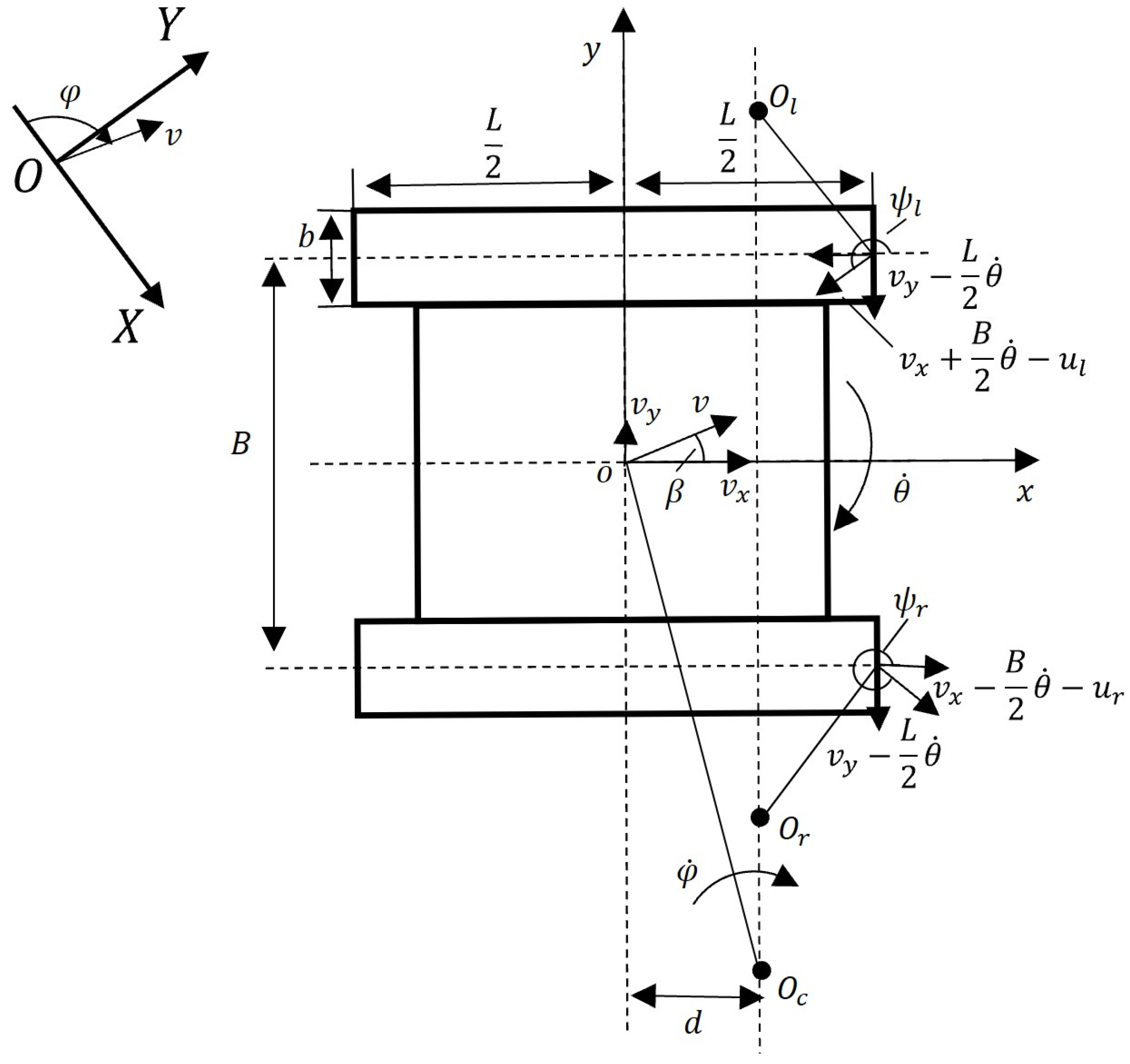
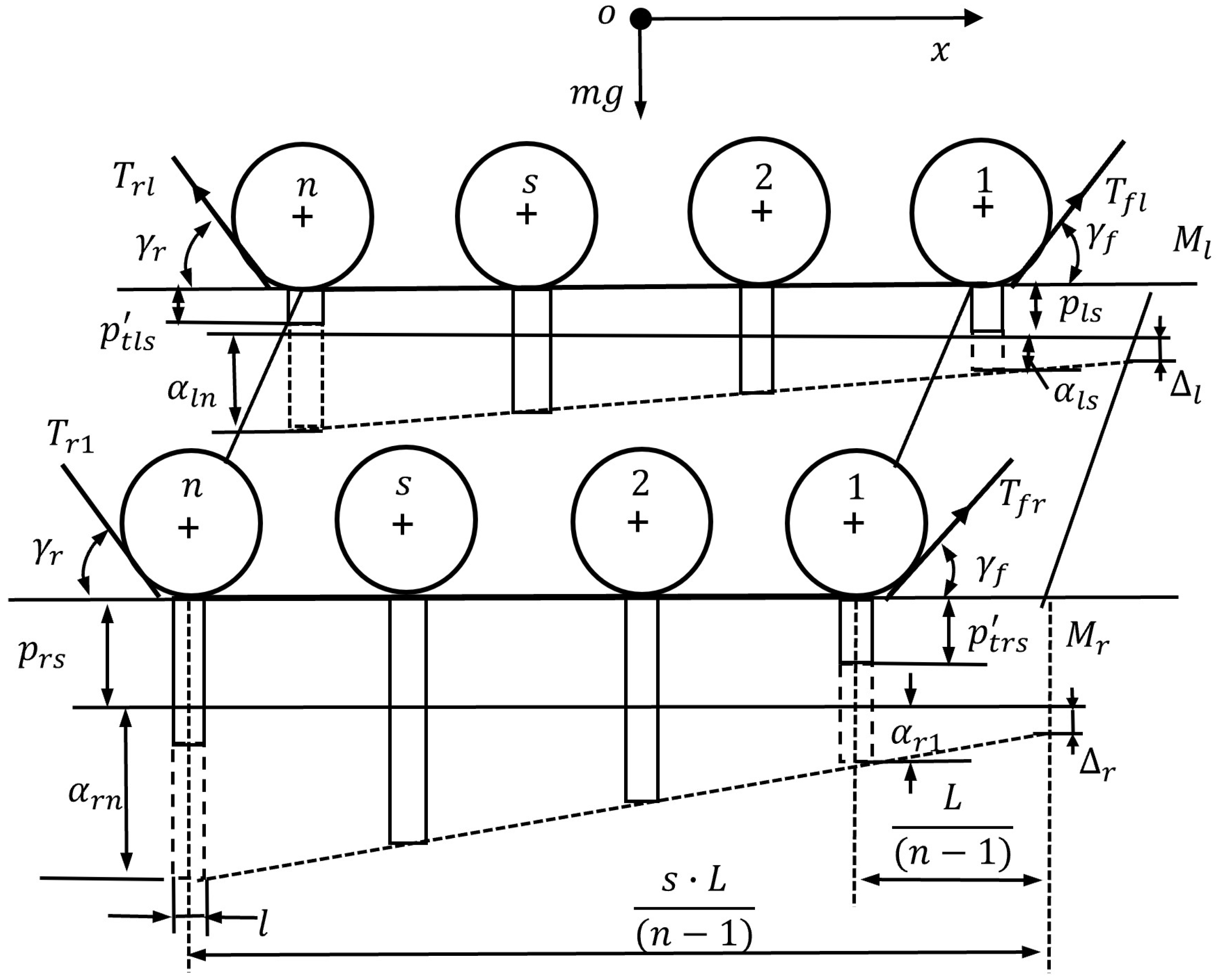
2.1. The Calculation of Shear Displacement in the Steering Process of a Tracked Vehicle

Taking a right turn made by the tracked vehicle as an example, the relationships between the motion parameters are shown in Figure 1.
The position coordinates in X O Y can be obtained by integrating the velocity of the center of mass according to Equation (2):
X = 0 t v cos θ β d t Y = 0 t v sin θ β d t .
The components and a y , can be expressed by Equation (3):
a x = v ˙ x + v y θ ˙ a y = v ˙ y v x θ ˙ .
Two points, x p , y p and ( x p , y p ), on the left and right tracks about x -axis symmetry were taken, respectively. By calculating the shear displacement of the two points, the relationship between the shear displacement of the track and the vehicle speed and yaw rate during the turning process was analyzed. The shear velocities, x s x l , v s x r , v s y l , and v s y r , of both tracks in the x - and y -directions at x p , y p and x p , y p can be expressed by Equation (4):
v s x l = v x + B 2 θ ˙ u l   v s x r = v x B 2 θ ˙ u r   v s y l = v s y r = v y x p θ ˙ .
The expression for the angles between the direction of velocity and the x -axis for the points x p , y p and x p , y p is:
ψ l = arccos v s x l v s x l 2 + v s y l 2 ψ r = arccos v s x r v s x l 2 + v s y l 2 .
The slip rate expression of the track on both sides, δ l and δ r , can be obtained as:
δ l = v s x l max u l + v s x l , u l δ r = v s x r max u r + v s x r , u r .
The shear displacements of two points are obtained by integrating the shear velocity of x p , y p and x p , y p according to Equations (7)–(9):
j x l = 0 t v s x l d t = v s x l u l L 2 x p j x r = 0 t v s x r d t = v s x r u r L 2 x p ,
j y l = 1 u l v y L 2 θ ˙ L 2 x p + 1 2 u l θ ˙ L 2 x p 2 j y r = 1 u r v y L 2 θ ˙ L 2 x p + 1 2 u r θ ˙ L 2 x p 2 ,
j l = j x l 2 + j y l 2 j r = j x r 2 + j y r 2 .

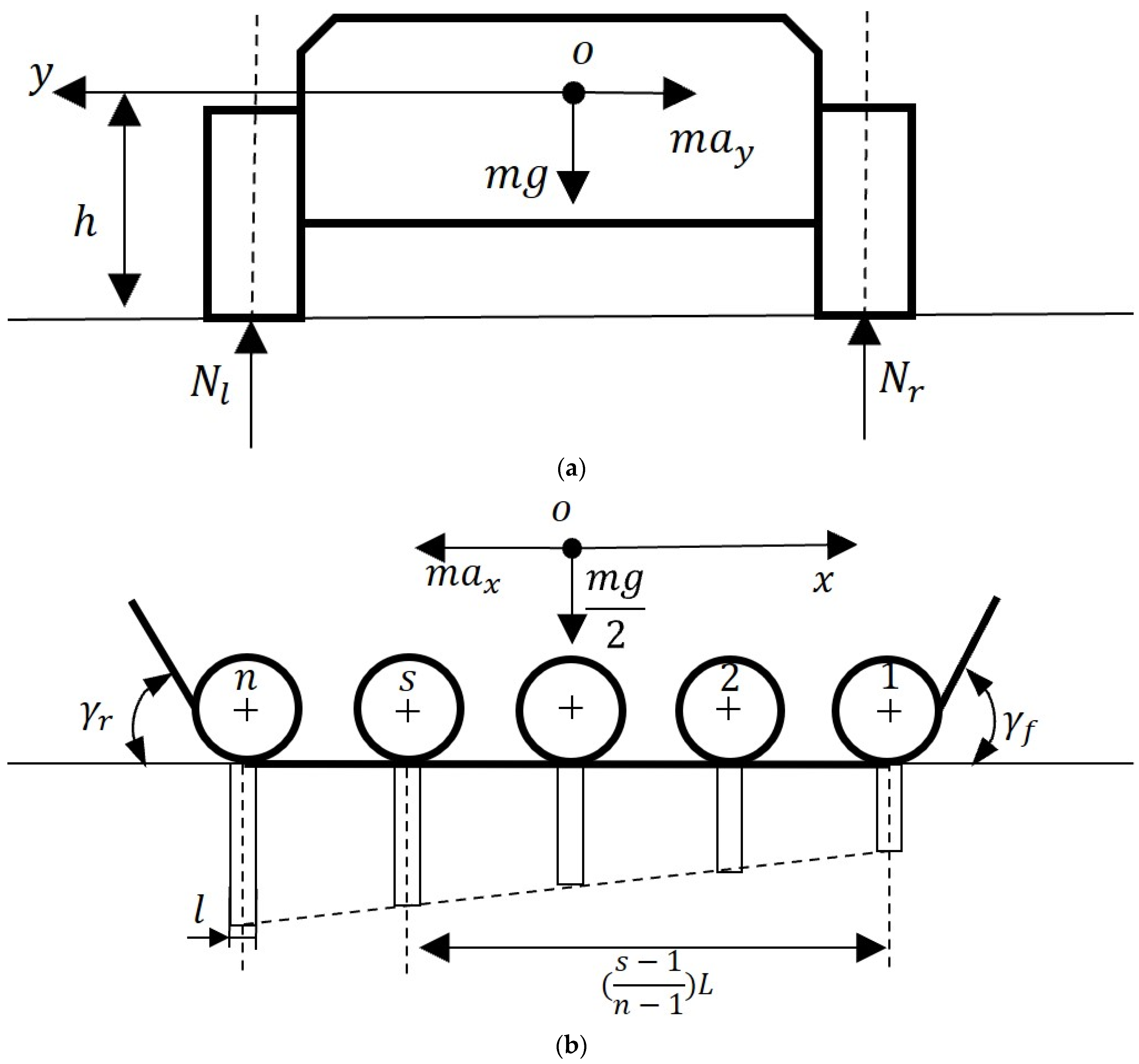
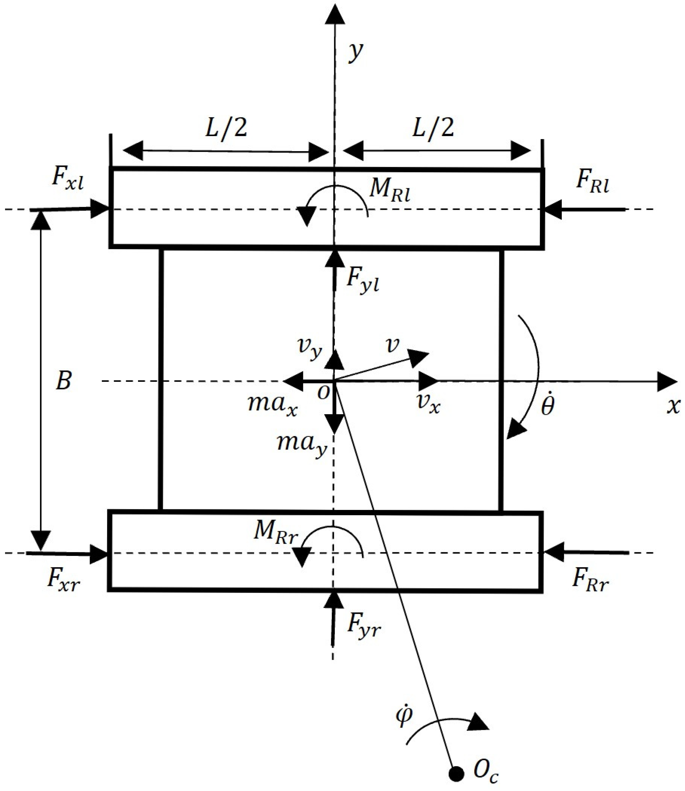
2.2. Tracked Vehicle Steering Force Analysis

The ground pressure distributions of both tracks directly impact the steering force of the tracked vehicle. The ground pressures, p l s and p r s , of the unit ground areas of the s t h load-bearing wheels of both tracks can be expressed by Equation (10):
p l s = p ¯ l s + p t l s p r s = p ¯ r s + p t r s .
In Equation (10), p l s and p r s represent the ground pressures of the unit ground areas of the load-bearing wheels on the left and right tracks, respectively, which are generated by the inertial and gravitational forces; p t l s and p t r s are the pressure changes of the unit ground areas of the s th load-bearing wheels on the both tracks, respectively.
Figure 2 shows the changes in the ground pressures of the load-bearing wheels, which are caused by the track tension. In this figure, M 1 M 2 is the auxiliary line used for solving for the steering force balance of the vehicle, which is at a distance of L / ( n + 1 ) from the front edge of the track ground plane.
During a right turn, the left track moves at a greater speed than the right track. The relationship between the tension and shear force of the tracks on both sides can be obtained by Equation (11):
T f l = F x l , T r l = 0 T r r = F x r , T f r = 0
The tension of the track has an effect on the first load wheel on the tension side in the vertical direction. For example, the expression of the ground pressure t l s of the s th load wheel of the left track is (Equation (12)):
t l 1 = T f l sin γ f t l 2 = t l 3 = t l n 1 = t l n = 0
The pressure variation, α l s , of the s th load-bearing wheel of the left track is linearly related to L and has a slope of k . Thus, α l s can be expressed by Equation (13):
α l s = k s L ( n 1 ) l b + Δ l
where Δ l represents the value of α l s at M 1 M 2 as it changes according to Equation (13).
The p t l s of the s t h load-bearing wheel of the left track can be obtained by combining Equations (11)–(13) into Equation (14):
p t l s = α l s , s 1 , s n   p t l 1 = α l 1 t l 1 / b l   p t l n = α l n t l n / b l   .
The moments of the forces of each load-bearing wheel on the left and right tracks with respect to the auxiliary line, M 1 M 2 , which are denoted as M l and M r , respectively, can be expressed by Equation (15):
M l = s = 1 n ( α l s + p l s ) · s L l b n 1 t l 1 · L n 1 t l n · n L n 1 M r = s = 1 n ( α r s + p r s ) · s L l b n 1 t r 1 · L n 1 t r n · n L n 1 .
A system of equations to describe the torque balance of the ground pressure of each load-bearing wheel on both tracks with respect to the auxiliary line was established and is presented as Equation (16):
M l + M r = m g ( L 2 + L n 1 ) s = 1 n ( α l s + p l s ) l b t l 1 t l n = s = 1 n ( α r s + p r s ) l b t r 1 t r n = m g 2 s = 1 n α l s = t l 1 + t l n s = 1 n α r s = t r 1 + t r n .
Expressions for p t l s and p t r s were obtained by combining Equations (11)–(16), and these expressions are presented in Equation (17):
p t l s = 3 t r 1 3 t r n 5 t l 1 t l n 2 n l b + 3 ( t r n + t l n t r 1 t l 1 ) s n ( n + 1 ) b l t l s / b l p t r s = 5 t r 1 t r n 3 t l 1 3 t l n 2 n l b + 3 ( t r n + t l n t r 1 t l 1 ) s n ( n + 1 ) b l t r s / b l  
The inertial force of the center of gravity affects the ground pressure distributions of both tracks during a tracked vehicle turning process. The inertial force affects the distribution of the ground pressure of each load wheel on both tracks, as shown in Figure 3.
Expressions for N l and N r are given in Equation (18):
N l = m g 2 m a y h B N r = m g 2 + m a y h B ,
The p ¯ l s and p ¯ r s of the s t h load-bearing wheels on both sides of the track can be expressed by Equation (19):
p ¯ l s = N l 3 2 s n 1 m a x h n n + 1 b l L , s = 1 n , p ¯ r s = N r 3 2 s n 1 m a x h n n + 1 b l L , s = 1 n , ,
The steering force of the tracked vehicle is illustrated in Figure 4. Equations (17)–(19) were combined to obtain expressions for the x - and y -components of the shear forces between the ground and both tracks, which are provided in Equations (20) and (21), respectively:
F x l = s = 1 n ( 3 s ) L 4 l 2 ( 3 s ) L 4 + l 2 b · c + p l s tan ϕ 1 e j x l K cos ψ l + π d x F x r = s = 1 n ( 3 s ) L 4 l 2 ( 3 s ) L 4 + l 2 b · c + p r s tan ϕ 1 e j x r K cos ψ r + π d x ,
F y l = s = 1 n ( 3 s ) L 4 l 2 ( 3 s ) L 4 + l 2 b · c + p l s tan ϕ 1 e j x l K sin ψ l + π d x F y r = s = 1 n ( 3 s ) L 4 l 2 ( 3 s ) L 4 + l 2 b · c + p r s tan ϕ 1 e j x r K sin ψ r + π d x .
The rolling resistances of both tracks can be expressed by Equation (22):
F R l = s = 1 n p l s f b l F R r = s = 1 n p r s f b l ,
The steering resistance torques of both tracks can be expressed by Equation (23):
M R l = s = 1 n ( 3 s ) L 4 l 2 ( 3 s ) L 4 + l 2 b · c + p l s tan ϕ 1 e j x l K sin ψ l + π x d x M R r = s = 1 n ( 3 s ) L 4 l 2 ( 3 s ) L 4 + l 2 b · c + p r s tan ϕ 1 e j x r K sin ψ r + π x d x .
A system of equations, provided in Equation (24), can describe the force relationship of the tracked vehicle during steering:
m a x = F x r + F x l F R l F R r m a y = F y r + F y l I z θ ¨ = B 2 ( F x l F x r ) B 2 ( F R l F R r ) M R r M R l .
The expressions for the x - and y -components of the tracked vehicle acceleration, which are denoted by v ˙ x   a n d   v ˙ y , respectively, and the yaw angular acceleration, θ ¨ , were obtained (Equation (25)):
v ˙ x = ( F x r + F x l F R r F R l ) / m v y θ ˙ v ˙ y = ( F y r + F y l ) / m + v x θ ˙ θ ¨ = ( B 2 ( F x l F x r ) B 2 ( F R l F R r ) M R 1 M R 2 ) / I z .

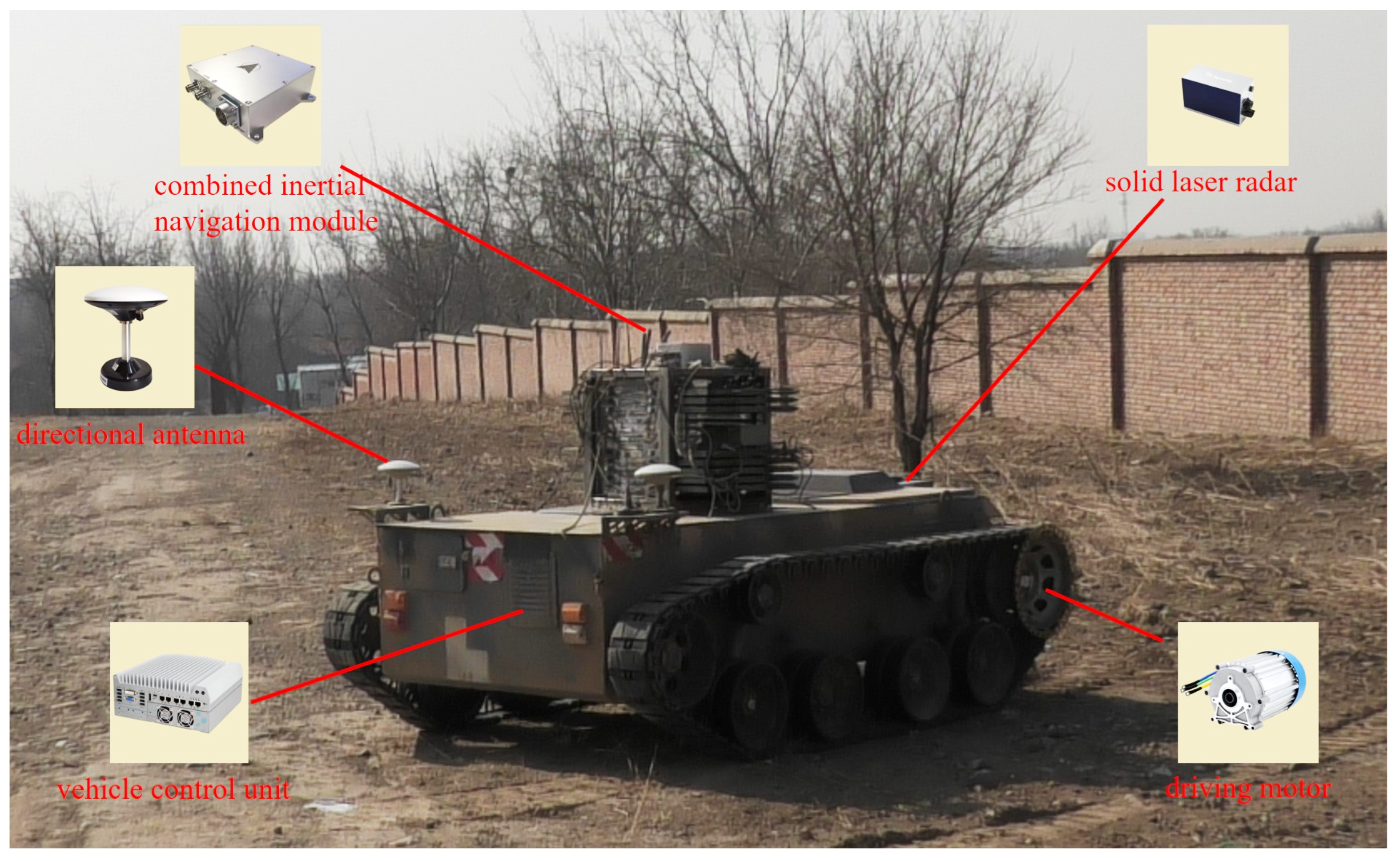
3. Experimental Verification

To verify the unmanned tracked vehicle position estimation accuracy of the dynamics model proposed in this paper, an experiment with an actual vehicle was designed. The tracked vehicle structural parameters and the road surface parameters are provided in Table 1. The experimental vehicle data acquisition system included a wheel speed sensor, a combined inertial navigation module, and a driving data recorder. The wheel speed sensor was installed at the sprockets to measure the circumferential velocities of both the left and right sprockets. The sprocket speed data of the tracked vehicle were used as the model input, and the vehicle position was estimated by using the steering dynamics and the kinematics model, respectively. The position estimation process is shown in Figure 5.
The positioning error of the combined inertial navigation module after the differential (GPS + RTK) is less than 2 cm , and the heading angle measurement error is less than 0.05 ° . The experimental vehicle is shown in Figure 6. The measurement information gathered from the combined inertial navigation module was assumed to be the actual position; this information was compared with the vehicle trajectories calculated by the tracked vehicle dynamics and kinematics models.

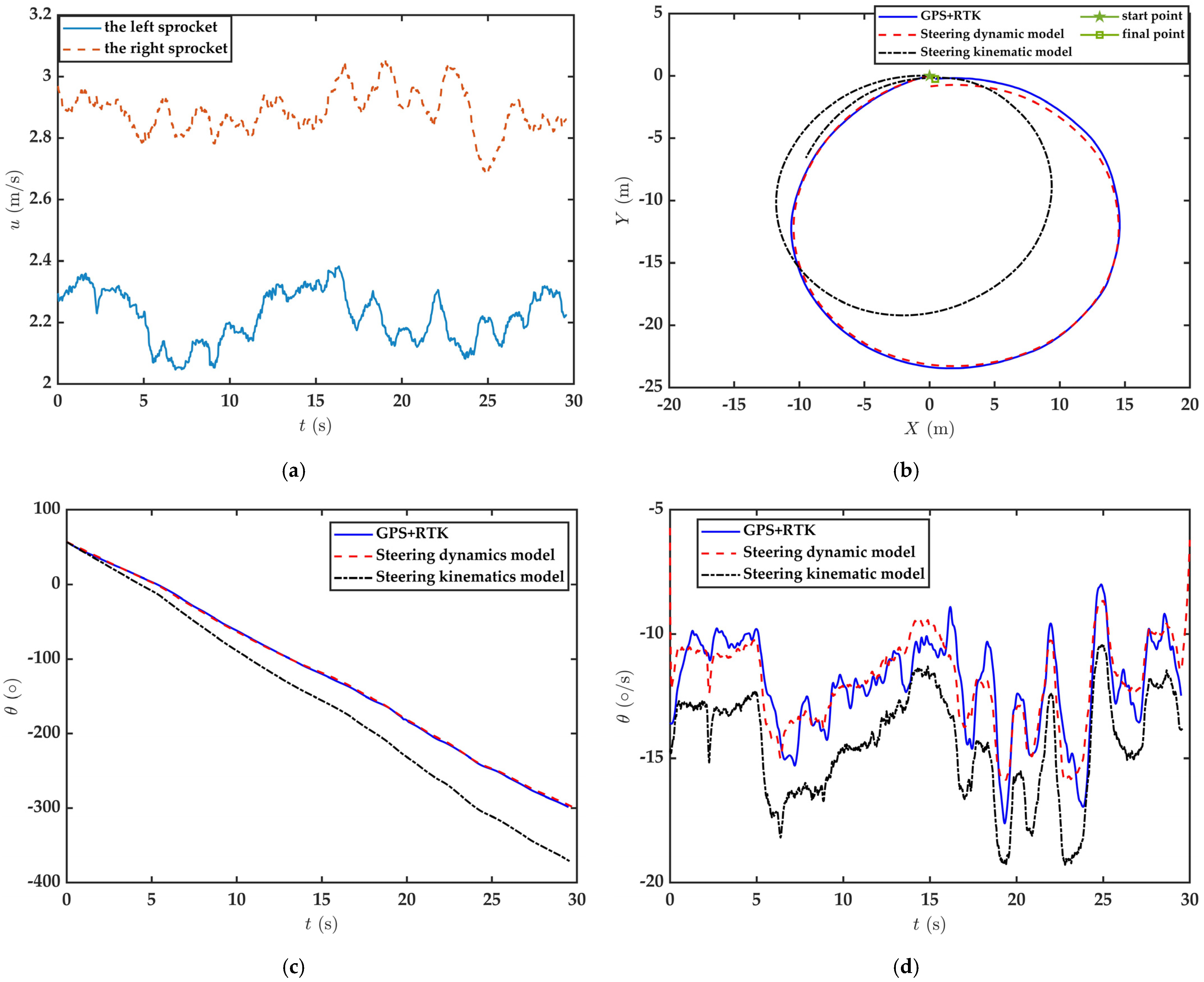
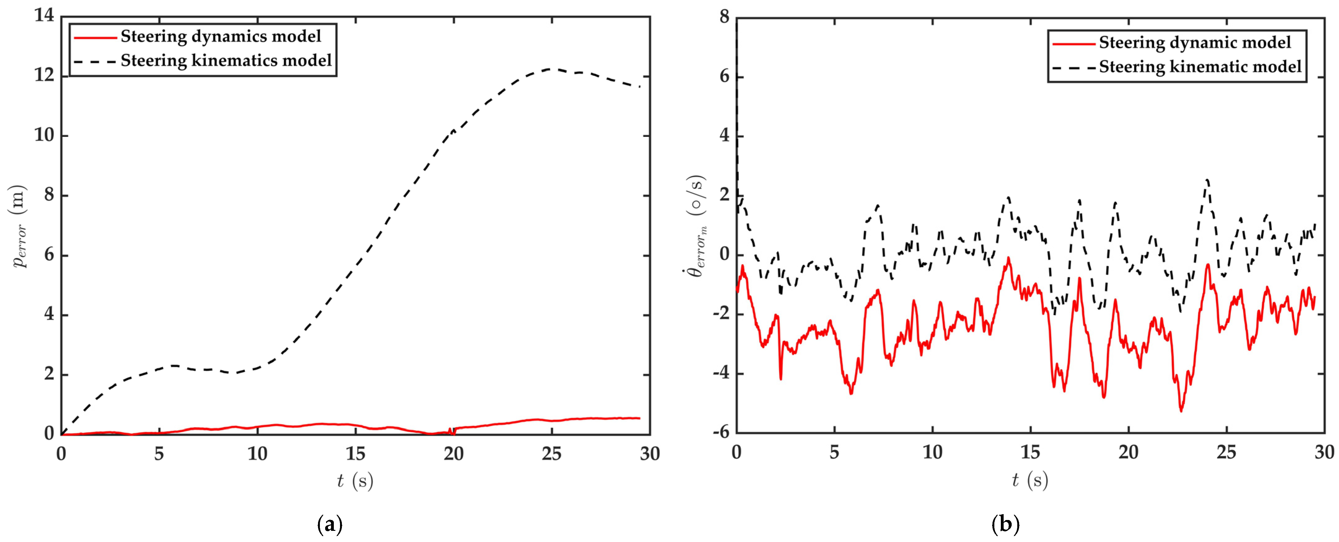
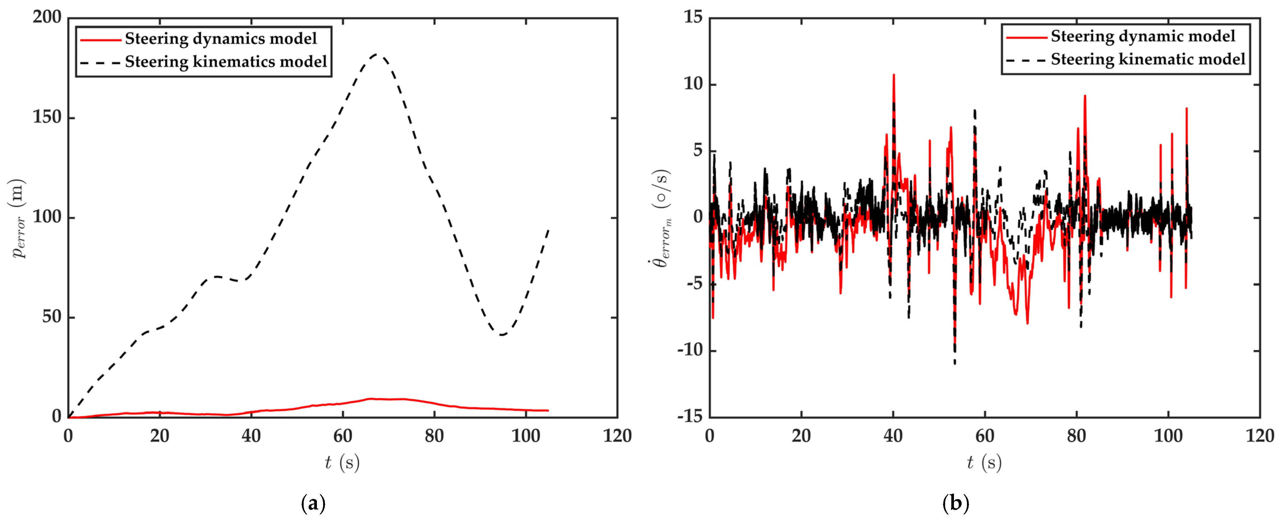
3.1. The Tracked Vehicle Performed Uniform Circular Motion on a Sand Road

The tracked vehicle performs uniform circular motion at different v t h . The v t h of the tracked vehicle is the average of the circumferential velocities of both sprockets: v t h = ( u l + u r ) / 2 . Figure 7 depicts the changes in the tracked vehicle state when it turned with a constant speed and a radius of 11.78   m on the sand road for one week. Figure 7a presents the velocity changes of the left and right sprockets. The average theoretical centroid velocity was 2.6   m / s during the entire turning process. Figure 7b shows the changes in the tracked vehicle steering trajectories. The tracked vehicle steered at a constant speed for one week, and the vehicle position estimated by the kinematics model had a large error compared with the actual position of the vehicle. The vehicle position estimated by the dynamics model was highly consistent with the actual position. Figure 7c depicts the changes in the heading angle during the tracked vehicle turning process. As the vehicle turned, the error in the heading angle calculated by the kinematics model gradually increased, reaching a maximum value of 72.35° at the end of the calculations. Figure 7d illustrates the changes in the yaw rate during the tracked vehicle turning process. Since sliding between the track and the ground during vehicle turning was not considered, the vehicle yaw rate calculated by the kinematics model was always greater than the actual yaw rate.
Figure 8 presents the trajectory and yaw rate errors for the tracked vehicle calculated by both the dynamics and kinematics models during the vehicle turning process. Figure 8a depicts the changes in the driving trajectory errors. The driving trajectory error calculated by the kinematics model exhibited a cumulative increasing trend with time, and the maximum error reached 12.24 m . The driving trajectory error calculated by the dynamics model was maintained at a low level and did not have a cumulative increasing trend. The maximum error for this case was 0.56 m . After the tracked vehicle continuously turned right for one week, the average trajectory error calculated by the kinematics model was p e r r o r _ m = 6.34   m . The average trajectory error calculated by the dynamics model, p e r r o r _ m = 0.263   m , was 95.85 % less than that calculated by the kinematics model. Figure 8b shows the changes in the yaw rate errors. The average yaw rate error calculated by the kinematics model was θ ˙ e r r o r _ m = 2.44 ° / s , and the fluctuations were stable. This result occurred because the tracked vehicle turned with a constant speed and a constant radius on a consistent road surface; thus, the slippage between the track and the ground changed little. The average yaw rate error calculated by the dynamics model was θ ˙ e r r o r _ m = 0.866 ° / s , which is a 64.5 % decrease from the value calculated by the kinematics model.
The tracked vehicle performed uniform circular steering with different v t h and R values on the sand road. The driving trajectory and yaw rate errors for these conditions are listed in Table 2, which demonstrates that the vehicle trajectory and yaw rate errors calculated by the dynamics model were significantly lower than those calculated by the kinematics model. The tracked vehicle performed 10 turning experiments on the sand road. The average yaw rate and trajectory tracking errors calculated by the kinematics model were θ ˙ e r r o r _ m = 2.14 ° / s and p e r r o r _ m = 11.08   m , respectively. The average yaw rate and trajectory tracking errors calculated by the dynamics model were θ ˙ e r r o r _ m = 0.325 ° / s and p e r r o r _ m = 1.71   m , respectively, which represent 84.8 % and 84.57 % decreases, respectively, from the values calculated by the kinematics model.

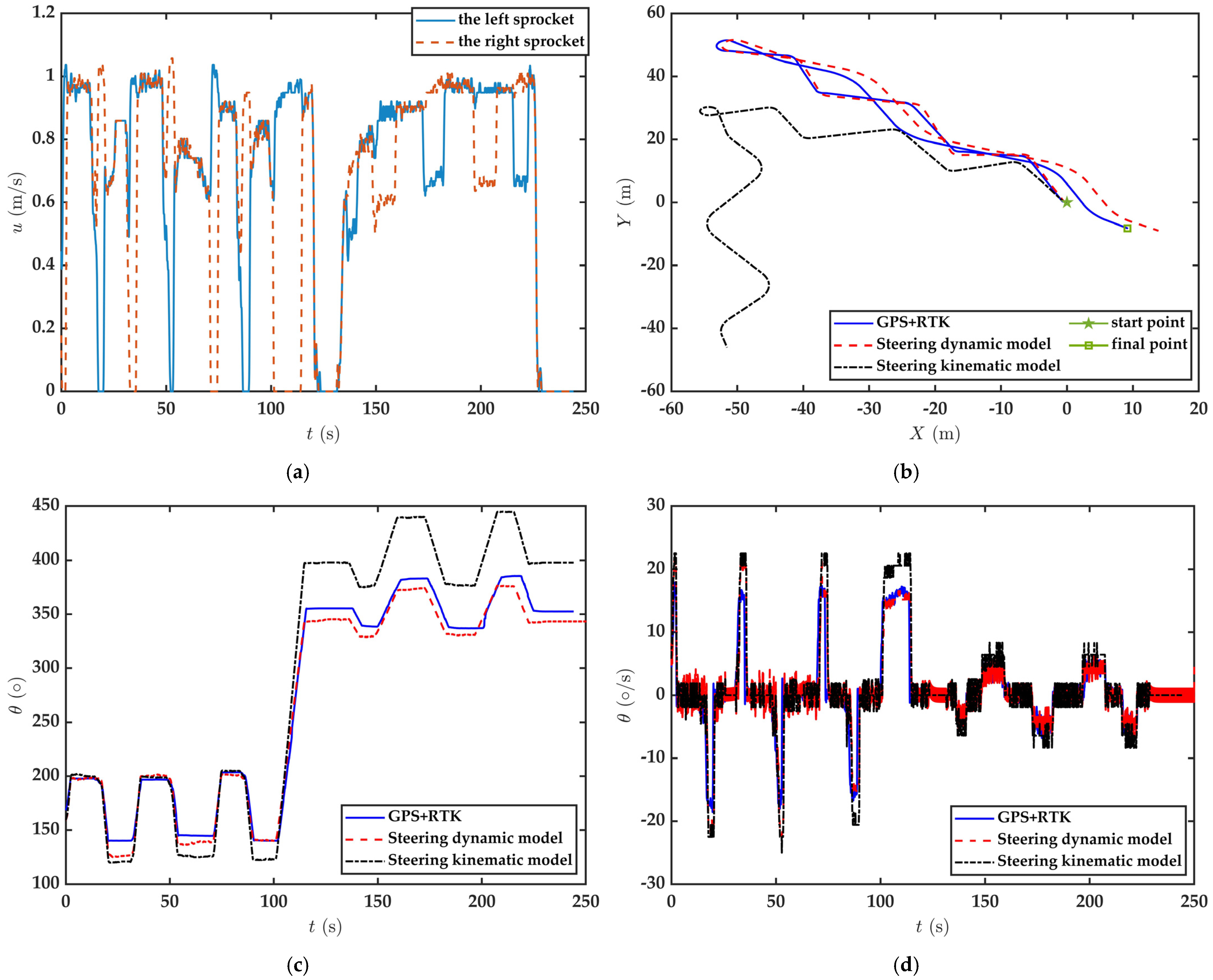
3.2. The Tracked Vehicle Performed General Turning Motion on a Sand Road

A driver drove the tracked vehicle on the sand road according to a predetermined trajectory, controlling the vehicle so that it performed acceleration, deceleration, and turning tasks that were based on the premise of ensuring driving safety. Figure 9 depicts the changes in the vehicle driving state during the whole driving process. Figure 9a presents the speed changes of the left and right sprockets. The driver adjusted both sprocket speeds in real time based on the predetermined trajectory to control the vehicle turning operations. The v ¯ t h of vehicle during the entire driving process was 4.62   m / s . Figure 9b depicts the changes of the position of the tracked vehicle. The total length of the trajectory was 491   m . The position estimated by the kinematics model was quite different from the actual trajectory of the vehicle, and it had a maximum error of 181.82   m . The dynamics model estimated that the vehicle position was in good agreement with the actual position, and the maximum error is only 9.41   m . Figure 9c illustrates the changes in the heading angle during the tracked vehicle turning process. The estimated heading angle of the kinematics model had a large error with the actual heading angle of the vehicle, and the maximum error is 74 ° . Figure 9d illustrates the changes in the yaw rate during the tracked vehicle turning process. The kinematics model did not consider the slippage between the track and the ground; thus, the yaw rate calculated by the kinematics model was always greater than the actual yaw rate. At t = 68.6   s , when the steering radius of the tracked vehicle was small, the yaw rate error reached 10.77   ° / s .
Figure 10 presents the changes in the trajectory and yaw rate errors during the entire tracked vehicle driving process. Figure 10a depicts the changes in the driving trajectory error. The average position error estimated by the kinematics model was 85.31 m . The average position error estimated by the dynamics model was 4.27 m , which is 95 % less than the position error estimated by the kinematics model. Figure 10b illustrates the changes in the estimation error of yaw rate during the tracked vehicle turning process. The average errors of yaw rate estimated by the kinematics model and the dynamics model are 0.66 ° / s and 0.044 ° / s , respectively. The trajectory and yaw rate errors estimated by the dynamics model were reduced by 95 % and 93.3 % , respectively.

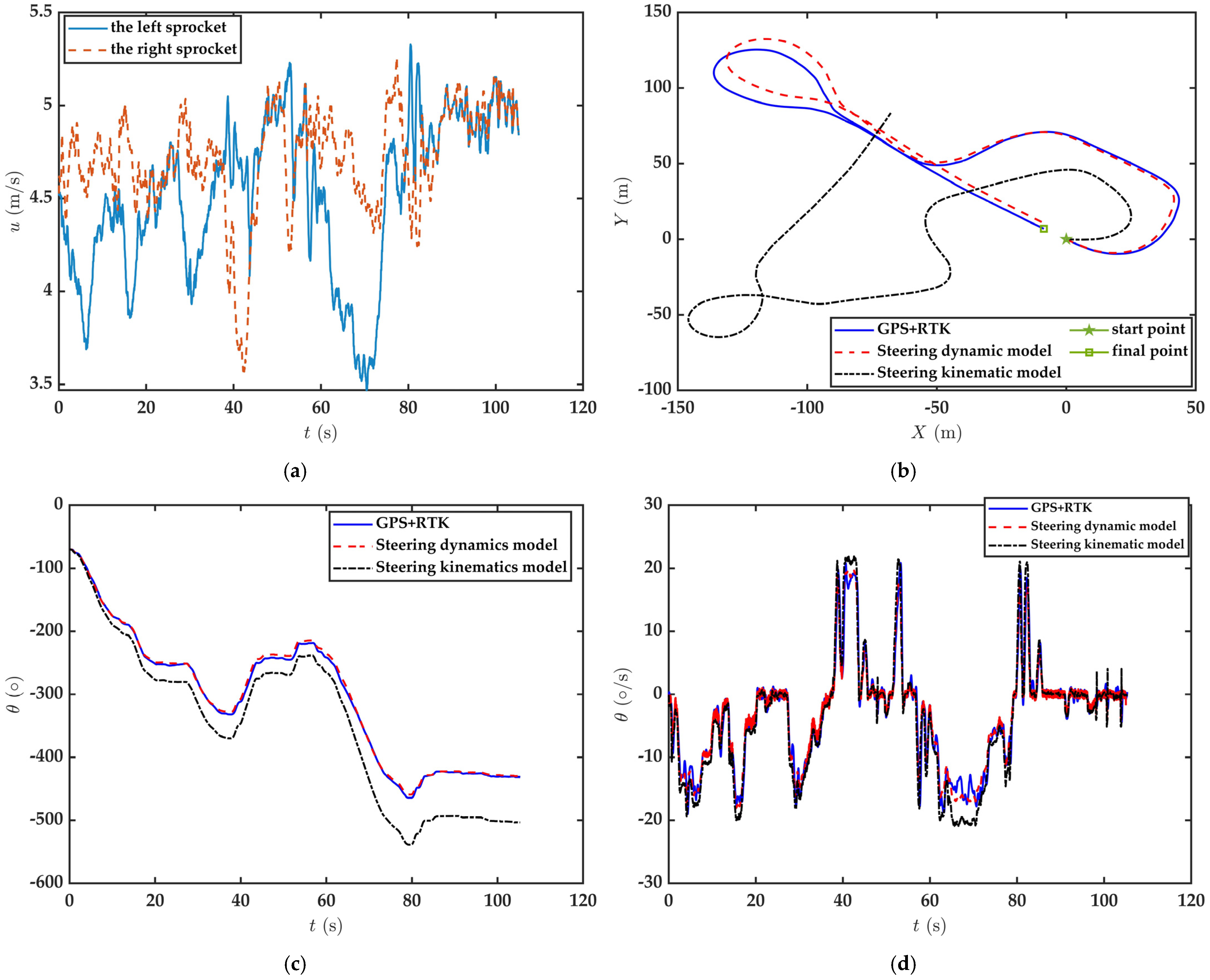
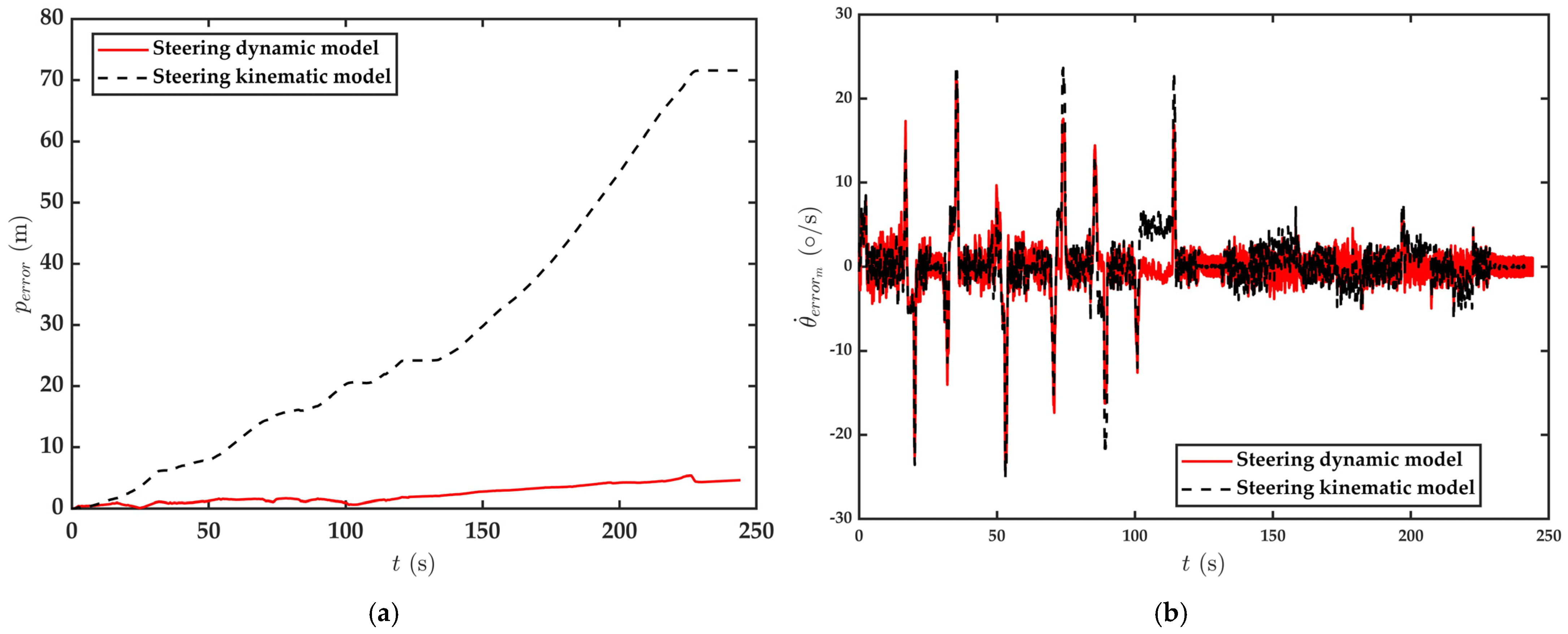
3.3. The Tracked Vehicle Performed Continuous Steering Motion on a Cement Pavement

The tracked vehicle performed continuous steering operation on the cement pavement. Because of the limitations of the experimental site, it was difficult to find a region of cement pavement that was wide enough for the tracked vehicle to perform turning operations with certain radii. The vehicle experiment was carried out on a long, straight cement runway. The tracked vehicle performed low-speed and small-radius continuous turning operations on the cement road. Figure 11 presents the changes in the vehicle parameters throughout the driving process. Figure 11a depicts the changes in the speeds of the left and right sprockets. An in situ driving mode, which featured braking by a single track in some sections, was adopted for the tracked vehicle. The duration of the entire driving process was 244   s , during which the average theoretical centroid speed was 0.68   m / s . Figure 11b shows the estimated position of the tracked vehicle. The driving position error estimated by the kinematics model gradually increased, reaching a maximum of 71.57   m by the end of the driving process. Figure 11c depicts the changes in the heading angle. For these cases of low-speed and small-radius turning, the heading angle error calculated by the kinematics model was large, with a maximum heading angle error of 57 ° . The heading angle error directly led to increases in the trajectory error. Figure 11d shows the changes in the yaw rate. When the in situ driving mode was employed, the slippage between the tracks and the ground was large even at low driving speeds, and the yaw rate error calculated by the kinematics model was large.
Figure 12 depicts the changes in the trajectory and yaw rate errors of the tracked vehicle when it performed continuous low-speed and small-radius turning operations on cement pavement. The average position errors estimated by the kinematics model and the dynamics model were 29.09   m and 2.31   m , respectively. The average errors of yaw rate estimated by the kinematics model and the dynamics model are 0.274 ° / s and 0.051 ° / s , respectively. The trajectory and yaw rate errors estimated by the dynamics model were reduced by 92.6 % and 81.39 % , respectively.

4. Conclusions

In the research process, a dynamics model that could be used for track position estimation was established. Three primary conclusions were drawn from the actual vehicle experiments performed during this study:
(1)
Using this steering dynamics model to estimate the position of a tracked vehicle produced a higher accuracy than utilizing the kinematics model. This method can provide a reference for unmanned tracked vehicles working in special environments that cannot use precise positioning systems.
(2)
The experimental results indicate that large errors are still produced when the dynamics model is used for tracked vehicle position estimations because the dynamics model ignores the effects of some factors, such as the road slope. Fully considering the effects of pavement parameters and improving the calculation accuracy of the dynamics model will be focal points of future research endeavors.
(3)
With the development of vehicle sensors, it is possible to measure some motion parameters of tracked vehicles, such as yaw angle, centroid velocity, and centroid sideslip angle. Therefore, it is also theoretically feasible to apply the dynamics model proposed in this paper to the trajectory tracking control of tracked vehicles for model prediction.

Author Contributions

Conceptualization, X.L. and C.Z.; methodology, W.J. and C.Z.; software, W.J. and D.X.; validation, W.J. and S.Z.; formal analysis, X.L.; investigation, D.X.; data curation, S.Z.; writing—original draft, X.L. and W.J.; writing—review and editing, W.J.; project administration, D.X. All authors have read and agreed to the published version of the manuscript.

Funding

This research received no external funding.

Data Availability Statement

The original contributions presented in the study are included in the article, further inquiries can be directed to the corresponding author.

Conflicts of Interest

The authors declare no conflict of interest.

Abbreviations

Notation
τ the shear stress
σ the ground pressure of the tracks
c the soil cohesion parameter
ϕ the soil internal friction angle
j the shear displacement
K the soil deformation parameter
x o y a body coordinate system
X O Y the geodetic coordinate system
v the centroid velocity
v x the velocity component of v in the x -axis direction
v y the velocity component of v in the y -axis direction
β the sideslip angle of the tracked vehicle
θ the yaw angle
φ the complementary angle of the angle between v and the x -axis
L the plane length of contact between track and ground
b the plane width of contact between track and ground
B the center line distance of the two sides of the track ground plane
ψ the angle between the direction of velocity of a point on the track and the x -direction
O l O r the instantaneous steering center of the tracks on both sides
O c the turning center
d the offset of O c relative to o in the x -direction
n the number of load-bearing wheels on one track
t l s t r s the vertical track tension components of the sth load-bearing wheels of the tracks on both sides
T f l T f r the front track tensions of the tracks on both sides
T r l T r r the rear track tensions of the tracks on both sides
γ f the approaching angle
γ r the departure angle
l the length of the ground pressure area of a single load-bearing wheel
N l N r the normal force exerted by the ground on both tracks
h the height of center of gravity
F x l F x r the component of the shear force in the x-direction
F y l F y r the component of the shear force in the y-direction
M R l M R r the steering resistance torques of the left and right tracks
F R l F R r the rolling resistances of the tracks on both sides
f the ground rolling resistance coefficient
I z the moment of inertia of the tracked vehicle
m the mass of the tracked vehicle
r the radius of the driving wheel

References

  1. Jiang, H.; Yan, C.; Li, Q.; Liang, L.; Li, J.; Tan, Y. Review of Static Stability of Self-propelled Agricultural Machinery. J. Xihua Univ. (Nat. Sci. Ed.) 2023, 42, 32–41. [Google Scholar]
  2. Tanyıldızı, A.K. Design, Control and Stabilization of a Transformable Wheeled Fire Fighting Robot with a Fire-Extinguishing, Ball-Shooting Turret. Machines 2023, 11, 492. [Google Scholar] [CrossRef]
  3. Atia, M.M.; Waslander, S.L. Map-aided adaptive GNSS/IMU sensor fusion scheme for robust urban navigation. Measurement 2019, 131, 615–627. [Google Scholar] [CrossRef]
  4. Pivarčiová, E.; Božek, P.; Turygin, Y.; Zajačko, I.; Shchenyatsky, A.; Václav, Š.; Císar, M.; Gemela, B. Analysis of control and correction options of mobile robot trajectory by an inertial navigation system. Int. J. Adv. Robot. Syst. 2018, 15, 1729881418755165. [Google Scholar] [CrossRef]
  5. Ulaş, C.; Temeltaş, H. 3D multi-layered normal distribution transform for fast and long range scan matching. J. Intell. Robot. Syst. 2013, 71, 85–108. [Google Scholar] [CrossRef]
  6. Cadena, C.; Carlone, L.; Carrillo, H.; Latif, Y.; Scaramuzza, D.; Neira, J.; Reid, I.D.; Leonard, J.J. Simultaneous localization and mapping: Present, future, and the robust-perception age. IEEE Trans. Robot. 2016, 32, 1039–1332. [Google Scholar] [CrossRef]
  7. Chen, S.; Liu, B.; Feng, C.; Vallespi-Gonzalez, C.; Wellington, C. 3d point cloud processing and learning for autonomous driving: Impacting map creation, localization, and perception. IEEE Signal Process. Mag. 2020, 38, 68–86. [Google Scholar] [CrossRef]
  8. Kong, J.; Pfeiffer, M.; Schildbach, G.; Borrelli, F. Kinematic and dynamic vehicle models for autonomous driving control design. In Proceedings of the 2015 IEEE Intelligent Vehicles Symposium (IV), Seoul, Republic of Korea, 28 June–1 July 2015; pp. 1094–1099. [Google Scholar]
  9. Pentzer, J.; Brennan, S.; Reichard, K. Model-based prediction of skid-steer robot kinematics using online estimation of track instantaneous centers of rotation. J. Field Robot. 2014, 31, 455–476. [Google Scholar] [CrossRef]
  10. Martínez, J.L.; Mandow, A.; Morales, J.; Garcia-Cerezo, A.; Pedraza, S. Kinematic modelling of tracked vehicles by experimental identification. In Proceedings of the 2004 IEEE/RSJ International Conference on Intelligent Robots and Systems (IROS) (IEEE Cat. No. 04CH37566), Sendai, Japan, 28 September–2 October 2004; Volume 2, pp. 1487–1492. [Google Scholar]
  11. Xiong, G.; Lu, H.; Guo, K.; Chen, H. Research on trajectory prediction of tracked vehicles based on real time slip estimation. Acta ArmamentarII 2017, 38, 600. [Google Scholar]
  12. Rogers-Marcovitz, F.; George, M.; Seegmiller, N.; Kelly, A. Aiding off-road inertial navigation with high performance models of wheel slip. In Proceedings of the 2012 IEEE/RSJ International Conference on Intelligent Robots and Systems, Algarve, Portugal, 7–12 October 2012; pp. 215–222. [Google Scholar]
  13. Moosavian, S.A.A.; Kalantari, A. Experimental slip estimation for exact kinematics modeling and control of a tracked mobile robot. In Proceedings of the 2008 IEEE/RSJ International Conference on Intelligent Robots and Systems, Nice, France, 22–26 September 2008; pp. 95–100. [Google Scholar]
  14. Min, H.; Wu, X.; Cheng, C.; Zhao, X. Kinematic and dynamic vehicle model-assisted global positioning method for autonomous vehicles with low-cost GPS/camera/in-vehicle sensors. Sensors 2019, 19, 5430. [Google Scholar] [PubMed]
  15. Purdy, D.J. A heuristic investigation into the design of a dynamic yaw controller for a high-speed tracked vehicle. Proc. Inst. Mech. Eng. Part D J. Automob. Eng. 2020, 234, 689–701. [Google Scholar] [CrossRef]
  16. Jing, C.; Wei, C.; Li, X.; Peng, Z. Test method of steering dynamic characteristics of differential steering mechanism of tracked vehicle. Trans. Chin. Soc. Agric. Eng. 2009, 25, 62–66. [Google Scholar]
  17. Wong, J.; Chiang, C. A general theory for skid steering of tracked vehicles on firm ground. Proc. Inst. Mech. Eng. Part D J. Automob. Eng. 2001, 215, 343–355. [Google Scholar] [CrossRef]
  18. Tang, S.; Yuan, S.; Hu, J.; Li, X.; Zhou, J.; Guo, J. Modeling of steady-state performance of skid-steering for high-speed tracked vehicles. J. Terramech. 2017, 73, 25–35. [Google Scholar] [CrossRef]
  19. Wang, H.; Chen, B.; Rui, Q.; Guo, J.; Shi, L.-C. Analysis and experiment of steady-state steering of tracked vehicle under concentrated load. Acta ArmamentarII 2016, 37, 2196. [Google Scholar]
  20. Özdemir, M.N.; Kılıç, V.; Ünlüsoy, Y.S. A new contact & slip model for tracked vehicle transient dynamics on hard ground. J. Terramech. 2017, 73, 3–23. [Google Scholar]
  21. Jia, W.; Liu, X.; Zhang, C.; Qiu, M.; Zhang, Y.; Quan, Q.; Sun, H. Research on Steering Stability of High-Speed Tracked Vehicles. Math. Probl. Eng. 2022, 2022, 4850104. [Google Scholar] [CrossRef]
Figure 1. Relationships between the tracked vehicle motion parameters during a right turn. Adapted from Ref. [21].
Wevj 15 00120 g001
Figure 2. Changes in the ground pressures caused by the track tension. Adapted from Ref. [21].
Wevj 15 00120 g002
Figure 3. The ground pressure distribution of each load wheel affected by inertial force: (a) the normal ground force on both tracks is affected by the inertial force; (b) the pressure of each load-bearing wheel on both tracks is affected by the inertial force. Adapted from Ref. [21].
Wevj 15 00120 g003
Figure 4. Steering force diagram for the tracked vehicle. Adapted from Ref. [21].
Wevj 15 00120 g004
Figure 5. Solution processes of the tracked vehicle position estimation simulation models that utilized (a) the dynamics model and (b) the kinematics model. Adapted from Ref. [21].
Wevj 15 00120 g005
Figure 6. The experimental vehicle.
Wevj 15 00120 g006
Figure 7. Changes in the state parameters of the tracked vehicle during uniform circular turning: (a) circumferential velocities of the left and right sprockets, (b) steering trajectory, (c) heading angle, and (d) yaw rate.
Wevj 15 00120 g007
Figure 8. Variations in the driving trajectory and yaw rate errors of the tracked vehicle: (a) driving trajectory errors and (b) yaw rate errors.
Wevj 15 00120 g008
Figure 9. Changes in the state parameters of the tracked vehicle: (a) circumferential velocities of the left and right sprockets, (b) driving trajectory, (c) heading angle, and (d) yaw rate.
Wevj 15 00120 g009
Figure 10. Variations in the trajectory and yaw rate errors: (a) driving position error and (b) yaw rate error.
Wevj 15 00120 g010
Figure 11. Changes in the state parameters of the tracked vehicle during small-radius continuous turning on a cement road: (a) circumferential velocities of the left and right sprockets, (b) driving trajectory, (c) heading angle, and (d) yaw rate.
Wevj 15 00120 g011
Figure 12. Changes in the driving trajectory and yaw rate errors: (a) driving trajectory error and (b) yaw rate error.
Wevj 15 00120 g012
Table 1. Vehicle structural parameters and road surface parameters.
Road Surface ParametersVehicle Structural Parameters
c (Pa)ϕ (°)m (kg)Iz (kg·m2)L (m)B (m)b (m)
1.331.113,00045002.781.640.28
K   ( cm ) f l   ( m ) r   ( m ) h   ( m ) n
1.20.0650.120.1831.0594
Table 2. θ ˙ e r r o r _ m and p e r r o r _ m calculation results when the tracked vehicle performed uniform circular steering experiments with different v t h and R values.
Experiment Number
v ¯ t h ( m / s )
R ( m )
Kinematics ModelDynamics Model
θ ˙ e r r o r _ m   ( ° / s )
p e r r o r _ m ( m )
θ ˙ e r r o r _ m   ( ° / s )
p e r r o r _ m ( m )
12.312.282.0365.7930.2781.172
22.611.242.446.340.8660.263
32.616.351.8617.460.072.97
42.618.121.7816.690.1031.52
52.618.51.6811.560.211.68
62.619.641.4612.330.2131.94
73.312.62.666.040.531.55
83.519.52.11130.342.12
93.612.83.217.650.571.61
103.720.32.1813.90.072.28
Disclaimer/Publisher’s Note: The statements, opinions and data contained in all publications are solely those of the individual author(s) and contributor(s) and not of MDPI and/or the editor(s). MDPI and/or the editor(s) disclaim responsibility for any injury to people or property resulting from any ideas, methods, instructions or products referred to in the content.

