BP-Adaptive PID Regulation for Constant Current and Voltage Control in WPT Systems

Abstract

To enhance the stability and disturbance rejection of wireless charging systems for electric vehicles, we designed a bilateral collaborative control strategy based on BP neural networks, achieving closed-loop constant voltage control for the secondary rectification circuit. Integrating BP neural network adaptive PID parameters with dual-phase-shift control, this strategy outperforms conventional incremental PID controllers in terms of response time and overshoot. Validated on an 11 kW experimental platform, our approach demonstrated efficient response under disturbances; with a load switch from 10 Ω to 12 Ω, the system exhibited a mere 5% fluctuation rate and an impressive efficiency of up to 92.96%.

1. Introduction

Today, low-carbon and environmentally friendly energy usage has become an area of active exploration in various fields. Reducing the proportion of oil and coal in the energy structure and developing new energy sources are effective approaches to addressing environmental energy issues [1,2,3]. In recent years, the use of electric vehicles (EVs) and plug-in hybrid electric vehicles (PHEVs) has been increasing. In comparison to traditional wired charging methods, wireless power transfer methods can effectively avoid mechanical wear, are not restricted by weather conditions, and typically involve underground placement of the emitting device, thus efficiently saving surface space. Additionally, they lack external exposed interfaces, offering higher safety and flexibility [4,5,6].

The existing control methods for wireless power transfer system in EVs can be broadly categorized into three classes: primary-side control, secondary-side control, and dual-side control. In primary-side control, a DC-DC section is typically introduced on the primary side, with BUCK, BOOST, CUK transformation circuits, etc. Alternatively, constant-frequency control techniques using high-frequency inverters, such as phase-shift control, can be employed. Secondary-side control involves controlling the output by connecting DC-DC converters or employing controllable rectifiers. Dual-side control is further divided into dual-side communication control and dual-side non-communication control. To minimize delays in wireless communication and reduce the introduction of energy conversion stages, the research focus is primarily on secondary-side control. Existing studies analyze various secondary-side control structures. In reference [7], a pair of bidirectional switches composed of MOSFETs was added between the compensation circuit and the rectifier bridge, resulting in eight possible operating states for the secondary side. The study also investigated the relationship between total harmonic distortion of the input current and the output voltage. Reference [8] proposed a secondary-side control method for an active rectifier with a dual LCC structure. The rectification section on the secondary side consists of two MOSFETs and two diodes. By analyzing the operation of the secondary-side circuit, a second order generalized integrator phase-locked loop generates a reference sine waveform. The phase difference, obtained through a comparison using the PI method, serves as the control variable, achieving higher-precision control of the secondary-side voltage. The system exhibits a faster dynamic response under load and line disturbances.

With the emergence of vehicle-to-grid (V2G) and grid-to-vehicle (G2V) technologies, bidirectional wireless power transfer is required. This technology relies on a symmetrical system structure and corresponding control methods on both sides, where the primary and secondary sides employ a full-bridge full-control structure to enable bidirectional energy transfer. Bac Yuan Nguyen et al. [9] implemented bilateral control of the system based on a symmetrical SS compensation topology. They designed a closed-loop controller and analyzed the losses of the coil and power converter, obtaining the conditions for obtaining the maximum efficiency of the system. However, this paper only implemented closed-loop control based on traditional methods. Boshen Zhang et al. [10] conducted a study on bidirectional control strategies for a dual LCC structure. Addressing the inherent frequency deviations between the gate signals of primary and secondary-side controllers, they introduced a novel dual-side LCC topology duty-cycle control scheme, specifically employing traditional phase-shift control on the primary side and duty-cycle control on the secondary side. Without the need for additional circuitry, this approach effectively mitigates synchronization issues in electric vehicle charging. However, it is worth noting that this method exhibits sensitivity to voltage fluctuations. F Liu et al. [11] conducted research on control strategies for a bidirectional WPT system with an SS structure, achieving efficiency optimization through a multi-degree-of-freedom combination control strategy. Additionally, Zhao S et al. [12] introduced a digital phase-synchronization method for bidirectional WPT systems, allowing for the extraction of active and reactive components of the AC current on the secondary side’s high-frequency converter. By adjusting the reactive current to zero, they synchronized the voltage phase of the secondary side’s high-frequency converter with that of the primary high-frequency converter.

In summary, conventional constant current-constant voltage charging methods are employed for the power batteries of EVs. However, this approach is associated with prolonged charging durations and suboptimal efficiency. Moreover, the magnetically coupled resonant wireless power transfer (MCRWPT) systems for electric vehicles are characterized by strong nonlinearity and complex multi-variable behavior [13,14,15], making conventional control strategies inadequate for addressing issues related to changes in internal resistance within the power batteries and deviations in the alignment of primary and secondary coils. Consequently, the exploration of innovative control strategies has become a focal point. Adjusting the output by controlling the primary-side inverter would require wireless communication for feedback regulation between the transmitting and receiving ends, leading to potential issues related to communication delays. Furthermore, the use of DC-DC converters on either the primary or secondary side for output regulation introduces energy conversion steps, resulting in additional losses [16,17,18,19,20]. Hence, there is room for improvement in the system response characteristics under traditional closed-loop control methods, as highlighted by existing research.

To address the aforementioned issues, this paper presents a bidirectional coordinated control strategy based on a symmetrical structure system. Initially, a dual-phase-shift control strategy was chosen as the control method for this system. The dual LCC structure is modeled, and a power converter loss model is established. The characteristics of the dual LCC circuit are utilized to achieve constant current control. Through an analysis of the relationship between phase-shift angles and output characteristics, a dual-phase-shift control strategy tailored to the MCRWPT system is designed, enabling high-efficiency bidirectional coordination control. Building upon the foundation of traditional PID control methods, this paper incorporates a BP neural network to update PID parameters, facilitating parameter-adaptive control and enhancing output stability in the presence of disturbances. The control strategy proposed in this paper not only satisfies the system’s output characteristics but also provides rapid, real-time response to significant disturbances during system operation and closed-loop control.

2. System Structure and Analysis

To facilitate bidirectional energy transfer between electric vehicle batteries and the electrical grid, the electric vehicle MCRWPT system adopts a symmetrical structure with primary and secondary sides, as illustrated in Figure 1.

In this configuration, Q₁~Q₈ represent MOSFET transistors. A direct current source is processed by the inverter circuit to generate a high-frequency square-wave voltage u_in. The red arrows show the direction of different currents. The primary side is composed of components L_f1, C_f1, C₁ and L_p, which together form the resonance network. The energy transfer coils are represented by L_p and L_s. The secondary side comprises components L_f2, C_f2, C₂ and L_s, creating a resonance network. The output of the dual LCC structure yields a sinusoidal current i_Lf2, which is rectified and filtered before being supplied to the battery load, R_L. It is important to note that the input of the dual LCC circuit can be equivalently represented as an AC source, U_in, and the output of the dual LCC circuit can be equivalently represented as a load, R_o, where R_o = 8R_L/π². Given its fully controllable mode, during forward energy transfer, the output load can be represented by the voltage U_L. The equivalent circuit is illustrated in Figure 2.

The model and analysis of the dual LCC topology circuit were conducted, resulting in expressions for the currents in the four mesh circuits, as follows:

$$\left[\begin{array}{c}{\mathrm{U}}_{\mathrm{in}}\\ 0\\ 0\\ 0\end{array}\right]=\left[\begin{array}{cccc}\mathrm{a}& \mathrm{b}& 0& 0\\ \mathrm{b}& \mathrm{c}& \mathrm{d}& 0\\ 0& \mathrm{d}& \mathrm{e}& \mathrm{f}\\ 0& 0& \mathrm{f}& \mathrm{g}\end{array}\right]\left[\begin{array}{c}{\mathrm{I}}_{\mathrm{Lf}1}\\ {\mathrm{I}}_1\\ {\mathrm{I}}_2\\ {\mathrm{I}}_{\mathrm{Lf}2}\end{array}\right]$$

(1)

where $\mathrm{a}=\mathrm{j}\mathsf{\omega }{\mathrm{L}}_{\mathrm{f}1}+\frac{1}{\mathrm{j}\mathsf{\omega }{\mathrm{C}}_{\mathrm{f}1}}$, $\mathrm{b} =\frac{1}{\mathrm{j}\mathsf{\omega }{\mathrm{C}}_{\mathrm{f}1}}$, $\mathrm{c}=\mathrm{j}\mathsf{\omega }{\mathrm{L}}_{\mathrm{p}}+\frac{1}{\mathrm{j}\mathsf{\omega }{\mathrm{C}}_{\mathrm{f}1}}+\frac{1}{\mathrm{j}\mathsf{\omega }{\mathrm{C}}_1}$, $\mathrm{d}=-\mathrm{j}\mathsf{\omega }\mathrm{M}$, $\mathrm{e}=\frac{1}{\mathrm{j}\mathsf{\omega }{\mathrm{C}}_2}+\mathrm{j}\mathsf{\omega }{\mathrm{L}}_2+\frac{1}{\mathrm{j}\mathsf{\omega }{\mathrm{C}}_{\mathrm{f}2}}$, $\mathrm{f}=\frac{1}{\mathrm{j}\mathsf{\omega }{\mathrm{C}}_{\mathrm{f}2}}$, $\mathrm{g}=\frac{1}{\mathrm{j}\mathsf{\omega }{\mathrm{C}}_{\mathrm{f}2}}+\mathrm{j}\mathsf{\omega }{\mathrm{L}}_{\mathrm{f}2}+{\mathrm{R}}_{\mathrm{o}}$. The resonance condition is as follows:

$$\left\{\begin{array}{c}\mathrm{j}{\mathsf{\omega }}_{\mathrm{o}}{\mathrm{L}}_{\mathrm{f}1}+\frac{1}{\mathrm{j}{\mathsf{\omega }}_{\mathrm{o}}{\mathrm{C}}_{\mathrm{f}1}}=0\\ \mathrm{j}{\mathsf{\omega }}_{\mathrm{o}}{\mathrm{L}}_{\mathrm{f}2}+\frac{1}{\mathrm{j}{\mathsf{\omega }}_{\mathrm{o}}{\mathrm{C}}_{\mathrm{f}2}}=0\\ \mathrm{j}{\mathsf{\omega }}_{\mathrm{o}}{\mathrm{L}}_1+\frac{1}{\mathrm{j}{\mathsf{\omega }}_{\mathrm{o}}{\mathrm{C}}_1}+\frac{1}{\mathrm{j}{\mathsf{\omega }}_{\mathrm{o}}{\mathrm{C}}_{\mathrm{f}1}}=0\\ \mathrm{j}{\mathsf{\omega }}_{\mathrm{o}}{\mathrm{L}}_2+\frac{1}{\mathrm{j}{\mathsf{\omega }}_{\mathrm{o}}{\mathrm{C}}_2}+\frac{1}{\mathrm{j}{\mathsf{\omega }}_{\mathrm{o}}{\mathrm{C}}_{\mathrm{f}2}}=0\end{array}\right.$$

(2)

where ω_o is the driving angular frequency.

Upon rearranging the above equation, we obtain the expression for the current phasor in the system’s resonant state as follows:

$$\left\{\begin{array}{c}{\mathrm{I}}_{\mathrm{Lf}1}=\frac{{\mathrm{U}}_{\mathrm{in}}{\mathrm{M}}^2{\mathrm{R}}_{\mathrm{o}}}{{\mathsf{\omega }}_{\mathrm{o}}^2{\mathrm{L}}_{\mathrm{f}1}^2{\mathrm{L}}_{\mathrm{f}2}^2}\angle 0°\\ {\mathrm{I}}_1=\frac{{\mathrm{U}}_{\mathrm{in}}}{{\mathsf{\omega }}_{\mathrm{o}}{\mathrm{L}}_{\mathrm{f}1}}\angle -90°\\ {\mathrm{I}}_2=\frac{{\mathrm{U}}_{\mathrm{in}}\mathrm{M}{\mathrm{R}}_{\mathrm{o}}}{{\mathsf{\omega }}_{\mathrm{o}}^2{\mathrm{L}}_{\mathrm{f}1}{\mathrm{L}}_{\mathrm{f}2}^2}\angle 0°\\ {\mathrm{I}}_{\mathrm{Lf}2}=\frac{{\mathrm{U}}_{\mathrm{in}}\mathrm{M}}{{\mathsf{\omega }}_{\mathrm{o}}{\mathrm{L}}_{\mathrm{f}1}{\mathrm{L}}_{\mathrm{f}2}}\angle -90°\end{array}\right.$$

(3)

3. Control Strategy

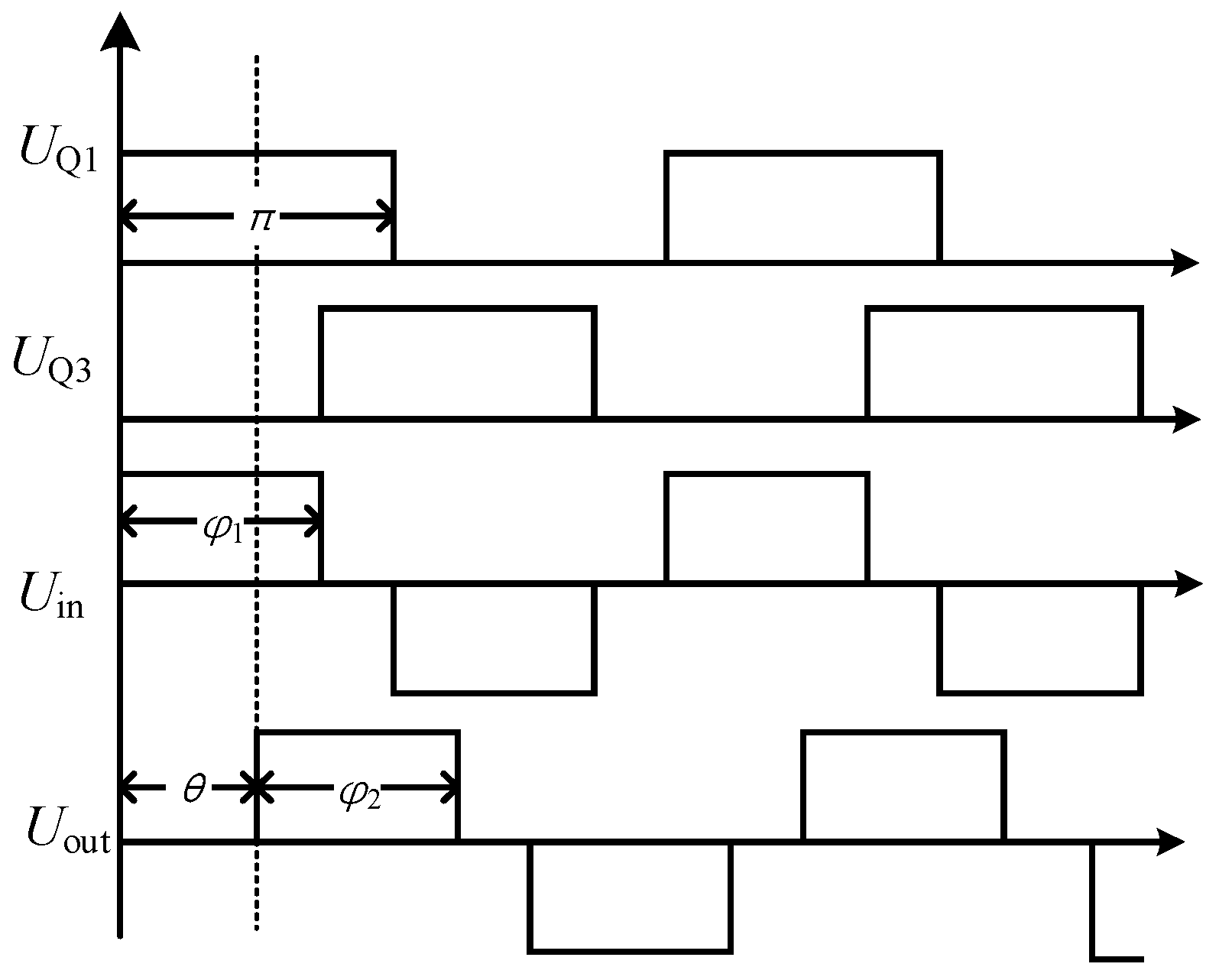
3.1. Dual-Phase-Shift Control Strategy Model

Figure 3 depicts voltage waveforms of triple-phase-shift control (TPS) [9]. When the phase angle θ between the primary and secondary sides is set to a constant value, it results in dual-phase-shift control (DPS) [20]. DPS control is achieved by manipulating two sets of converter phase-shift angles to mitigate power backflow and current stress in the system. The specific structure of the dual-phase-shift MCRWPT system is illustrated in Figure 1 above. U_Q1~U_Q8 represent the trigger signal waveforms for eight MOSFETs within the converters. U_in corresponds to the output voltage of the primary-side inverter, while U_out represents the input voltage of the secondary-side rectifier. φ₁ stands for the inverter phase-shift angle, φ₂ denotes the rectifier phase-shift angle, and θ indicates the phase difference between the primary and secondary sides. Each switch conducts for 180°, and the switching states of the upper and lower switches on the same bridge arm are complementary. When adjacent switches on the same converter’s two bridge arms conduct simultaneously, the corresponding U_in or U_out becomes zero. Conversely, when the adjacent switches conduct with opposite states, the power source voltage is generated. A larger phase-shift angle results in a higher effective value of terminal voltage.

Based on the principles of dual-phase-shift control, and in conjunction with the system model described earlier, we can derive the amplitude expressions for the input voltage U_in and the output voltage U_out as follows:

$${\mathrm{U}}_{\mathrm{in}}=\frac{4{\mathrm{U}}_{\mathrm{s}}}{\pi }{\displaystyle \sum _{\mathrm{n}=1,3,\dots }^{\infty }\frac{1}{\mathrm{n}}} \cos (\mathrm{n}{\mathsf{\omega }}_{\mathrm{o}}\mathrm{t}) \sin (\frac{\mathrm{n}{\mathsf{\phi }}_1}{2})$$

(4)

$${\mathrm{U}}_{\mathrm{out}}=\frac{4{\mathrm{U}}_{\mathrm{L}}}{\pi }{\displaystyle \sum _{\mathrm{n}=1,3,\dots }^{\infty }\frac{1}{\mathrm{n}}} \cos (\mathrm{n}{\mathsf{\omega }}_{\mathrm{o}}\mathrm{t}+\mathrm{n}\mathsf{\theta }) \sin (\frac{\mathrm{n}{\mathsf{\phi }}_2}{2})$$

(5)

Then, the phasors U_in and U_out can be expressed as follows:

$${\mathrm{U}}_{\mathrm{in}}=\frac{2\sqrt{2}{\mathrm{U}}_{\mathrm{s}}}{\pi }\sin (\frac{{\mathsf{\phi }}_1}{2})\angle 0°$$

(6)

$${\mathrm{U}}_{\mathrm{out}}=\frac{2\sqrt{2}{\mathrm{U}}_{\mathrm{L}}}{\pi }\sin (\frac{{\mathsf{\phi }}_2}{2})\angle \mathsf{\theta }$$

(7)

By combining the preceding derivation and rearranging the equation, we arrive at the expression for the current phasor in the system’s resonant state as follows:

$$\left\{\begin{array}{c}{\mathrm{I}}_1=\frac{{\mathrm{U}}_{\mathrm{in}}}{{\mathsf{\omega }}_{\mathrm{o}}{\mathrm{L}}_{\mathrm{f}1}}\angle -90°=\frac{{\mathrm{U}}_{\mathrm{in}}}{\mathrm{j}{\mathsf{\omega }}_{\mathrm{o}}{\mathrm{L}}_{\mathrm{f}1}}\\ {\mathrm{I}}_{\mathrm{Lf}2}=\frac{\mathrm{M}{\mathrm{U}}_{\mathrm{in}}}{{\mathsf{\omega }}_{\mathrm{o}}{\mathrm{L}}_{\mathrm{f}1}{\mathrm{L}}_{\mathrm{f}2}}\angle -90°=\frac{\mathrm{M}{\mathrm{U}}_{\mathrm{in}}}{\mathrm{j}{\mathsf{\omega }}_{\mathrm{o}}{\mathrm{L}}_{\mathrm{f}1}{\mathrm{L}}_{\mathrm{f}2}}\\ {\mathrm{I}}_{\mathrm{Lf}1}=\frac{\mathrm{M}{\mathrm{U}}_{\mathrm{out}}}{{\mathsf{\omega }}_{\mathrm{o}}{\mathrm{L}}_{\mathrm{f}1}{\mathrm{L}}_{\mathrm{f}2}}\angle 90°=\frac{\mathrm{jM}{\mathrm{U}}_{\mathrm{out}}}{{\mathsf{\omega }}_{\mathrm{o}}{\mathrm{L}}_{\mathrm{f}1}{\mathrm{L}}_{\mathrm{f}2}}\\ {\mathrm{I}}_2=\frac{{\mathrm{U}}_{\mathrm{out}}}{{\mathsf{\omega }}_{\mathrm{o}}{\mathrm{L}}_{\mathrm{f}2}}\angle 90°=\frac{\mathrm{j}{\mathrm{U}}_{\mathrm{out}}}{{\mathsf{\omega }}_{\mathrm{o}}{\mathrm{L}}_{\mathrm{f}2}}\end{array}\right.$$

(8)

The current amplitude is:

$$\left\{\begin{array}{c}{\mathrm{I}}_1=-\frac{2\sqrt{2}{\mathrm{U}}_{\mathrm{s}}}{\pi {\mathsf{\omega }}_{\mathrm{o}}{\mathrm{L}}_{\mathrm{f}1}}\sin ({\mathsf{\omega }}_{\mathrm{o}}\mathrm{t}\left)\sin \right(\frac{{\mathsf{\phi }}_1}{2})\\ {\mathrm{I}}_{\mathrm{Lf}2}=-\frac{2\sqrt{2}\mathrm{M}{\mathrm{U}}_{\mathrm{s}}}{\pi {\mathsf{\omega }}_{\mathrm{o}}{\mathrm{L}}_{\mathrm{f}1}{\mathrm{L}}_{\mathrm{f}2}}\sin ({\mathsf{\omega }}_{\mathrm{o}}\mathrm{t}\left)\sin \right(\frac{{\mathsf{\phi }}_1}{2})\\ {\mathrm{I}}_{\mathrm{Lf}1}=-\frac{2\sqrt{2}\mathrm{M}{\mathrm{U}}_{\mathrm{L}}}{\pi {\mathsf{\omega }}_{\mathrm{o}}{\mathrm{L}}_{\mathrm{f}1}{\mathrm{L}}_{\mathrm{f}2}}\sin ({\mathsf{\omega }}_{\mathrm{o}}\mathrm{t}+\mathsf{\theta }\left)\sin \right(\frac{{\mathsf{\phi }}_2}{2})\\ {\mathrm{I}}_2=-\frac{2\sqrt{2}{\mathrm{U}}_{\mathrm{L}}}{\pi {\mathsf{\omega }}_{\mathrm{o}}{\mathrm{L}}_{\mathrm{f}2}}\sin ({\mathsf{\omega }}_{\mathrm{o}}\mathrm{t}+\mathsf{\theta }\left)\sin \right(\frac{{\mathsf{\phi }}_2}{2})\end{array}\right.$$

(9)

Hence, we can derive the expressions for the input power P_out of the secondary-side rectifier. The expressions for the AC-side power, neglecting line resistance and circuit parameter deviations, are as follows:

$${\mathrm{P}}_{\mathrm{out}}=\frac{\mathrm{M}{\mathrm{U}}_{\mathrm{in}}{\mathrm{U}}_{\mathrm{out}}}{{\mathsf{\omega }}_{\mathrm{o}}{\mathrm{L}}_{\mathrm{f}1}{\mathrm{L}}_{\mathrm{f}2}}$$

(10)

where the expressions for U_in and U_out are given by (6) and (7) as shown, the circuit operates at the resonant frequency. When θ is set at +/−90°, the reactive power component becomes zero, and the power reaches its maximum. In the range of θ from −180° to 0°, power flows in the forward direction, while in the range of θ from 0° to 180°, power flows in the reverse direction. According to (10), adjusting the phase-shift angles on the primary and secondary sides as well as the phase difference in voltage between the two sides can be used to control the power. Changing the phase-shift angle on the secondary side can adjust the output voltage, while the output current on the secondary side can only be adjusted through the phase-shift angle on the primary side, thus validating the constant current source characteristic of the double LCC circuit. In the following sections, we will build upon this foundation to design a dual-side control strategy, aiming to achieve the high-efficiency operation of the system.

3.2. Controller Structure

Figure 4 illustrates the control structure, where the input to the BP neural network is set as the reference value r, the output value y, and the error e. The outputs are k_p, k_i, and k_d, corresponding to the three coefficients from the output layer as shown in Figure 5. The PID method [21,22,23,24] is employed to achieve closed-loop control of the system, with its output u(k) serving as the phase-shift angle control signal for the full-bridge rectifier or full-bridge inverter. By adjusting the phase-shift angle on the secondary side, a constant voltage control mode is achieved. The function u(k) is a function that depends on PID coefficients and errors, and it can be trained through a BP neural network to establish the optimal control rules, allowing for adaptive adjustment of PID parameters based on changes in the system’s operational state. The incremental digital PID formula is as follows:

$$\mathrm{u}\left(\mathrm{k}\right)=\mathrm{u}(\mathrm{k}-1)+{\mathrm{k}}_{\mathrm{p}}\left[\mathrm{e}\right(\mathrm{k})-\mathrm{e}(\mathrm{k}-1\left)\right]+{\mathrm{k}}_{\mathrm{i}}\mathrm{e}\left(\mathrm{k}\right)+{\mathrm{k}}_{\mathrm{d}}\left[\mathrm{e}\right(\mathrm{k})-2\mathrm{e}(\mathrm{k}-1)+\mathrm{e}(\mathrm{k}-2\left)\right]$$

(11)

The BP neural network [25,26] employs a three-layer structure, as illustrated in Figure 5. Since the output consists of three parameters that are non-negative, it is advisable to choose a non-negative sigmoid function for the activation functions in the output layer. As for the hidden layer, a symmetrical sigmoid function, which can take both positive and negative values, can be employed.

3.3. Subsection

Based on the structure of the BP neural network, as depicted in Figure 5, the calculations are performed. First, we define superscripts (1), (2), and (3) to represent the input layer, hidden layer, and output layer, as shown in detail in

Table 1. Relationship equations for the input layer, hidden layer, and output layer.

Input Layer	Hidden Layer	Output Layer
${\mathrm{O}}_{\mathrm{j}}^{\left(1\right)}=\mathrm{x}\left(\mathrm{j}\right){,}_{}^{}\mathrm{j}=1,2,3$   (12)	${\mathrm{net}}_{\mathrm{i}}^{\left(2\right)}\left(\mathrm{k}\right)={\displaystyle \sum _{\mathrm{j}=0}^3{\mathrm{w}}_{\mathrm{ij}}^{\left(2\right)}}{\mathrm{O}}_{\mathrm{j}}^{\left(1\right)}\left(\mathrm{k}\right){,}_{}^{}(\mathrm{i}=1,2,\dots ,\mathrm{q})$  (13)	${\mathrm{net}}_{\mathrm{l}}^{\left(3\right)}\left(\mathrm{k}\right)={\displaystyle \sum _{\mathrm{i}=1}^{\mathrm{Q}}{\mathrm{w}}_{\mathrm{li}}^{\left(3\right)}}{\mathrm{O}}_{\mathrm{i}}^{\left(2\right)}\left(\mathrm{k}\right)$    (16)
	${\mathrm{O}}_{\mathrm{i}}^{\left(2\right)}\left(\mathrm{k}\right)=\mathrm{f}[{\mathrm{net}}_{\mathrm{i}}^{\left(2\right)}\left(\mathrm{k}\right)]$          (14)	${\mathrm{O}}_{\mathrm{l}}^{\left(3\right)}\left(\mathrm{k}\right)=\mathrm{g}[{\mathrm{net}}_{\mathrm{l}}^{\left(3\right)}\left(\mathrm{k}\right)]{,}_{}^{}(\mathrm{l}=1,2,3)$ (17)
	$\mathrm{f}\left(\mathrm{x}\right)=\tan \mathrm{h}\left(\mathrm{x}\right)=\frac{{\mathrm{e}}^{\mathrm{x}}-{\mathrm{e}}^{-\mathrm{x}}}{{\mathrm{e}}^{\mathrm{x}}+{\mathrm{e}}^{-\mathrm{x}}}$        (15)	$\mathrm{g}\left(\mathrm{x}\right)=\frac{1}{2}(1+\tan \mathrm{h}(\mathrm{x}\left)\right)=\frac{{\mathrm{e}}^{\mathrm{x}}}{{\mathrm{e}}^{\mathrm{x}}+{\mathrm{e}}^{-\mathrm{x}}}$ (18)

.

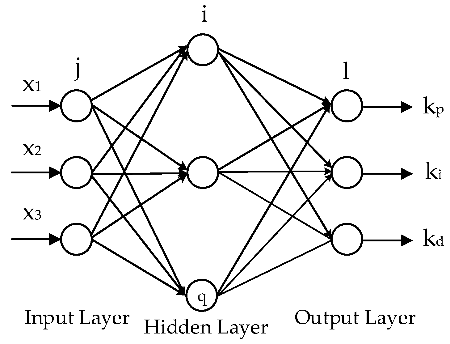
3.3.1. Neural Network Input Layer

The output of the input layer is denoted as ${\mathrm{O}}_{\mathrm{j}}^{\left(1\right)}$, where j represents the number of inputs. Next, we will provide a detailed explanation of the model derivation and weight update process for the hidden layer and the output layer.

3.3.2. Second Item; Neural Network Hidden Layer

Let us write down the input and output for the hidden layer separately. The input of each node in the hidden layer is the sum of the product of each output from the input layer and its corresponding weight. The input of the hidden layer, denoted as ${\mathrm{net}}_{\mathrm{i}}^{\left(2\right)}\left(\mathrm{k}\right)$, is subjected to an activation function to obtain the output, which is expressed as ${\mathrm{O}}_{\mathrm{i}}^{\left(2\right)}\left(\mathrm{k}\right)$. Here, q represents the number of nodes in the hidden layer, and ${\mathrm{w}}_{\mathrm{ij}}^{\left(2\right)}$ represents the weight coefficients directly connecting the input layer to the hidden layer, which totals 3q. The activation function employed is the hyperbolic tangent function, a symmetric sigmoid function, with the functional form denoted as f(x).

3.3.3. Neural Network Output Layer

Then, attention is turned to the output layer. The input to the output layer is obtained by multiplying the output of each node in the hidden layer by their respective weights and summing them up. Similarly, the expressions for the input and output of the output layer are denoted as ${\mathrm{net}}_{\mathrm{l}}^{\left(3\right)}\left(\mathrm{k}\right)$ and ${\mathrm{O}}_{\mathrm{l}}^{\left(3\right)}\left(\mathrm{k}\right)$. Here, l represents the number of output variables, and ${\mathrm{w}}_{\mathrm{li}}^{\left(3\right)}$ represents the weight coefficients directly connecting the hidden layer to the output layer, totaling 3q. The activation function for the output layer nodes is the sigmoid function, which is non-negative, and its expression is represented as g(x).

3.3.4. Weight Update

Using the square of the output error as a performance metric, the performance metric function is represented as E(k):

$$\mathrm{E}\left(\mathrm{k}\right)=\frac{1}{2}{[\mathrm{r}\left(\mathrm{k}+1\right)-\mathrm{y}(\mathrm{k}+1)]}^2$$

(19)

We employ the gradient descent method to recompute and adjust the weighting coefficients of the entire neural network. To ensure rapid convergence to a global minimum during the search, an inertia term is included. Thus, we obtain the weight correction formula for the output layer of the BP neural network, as represented by $\mathsf{\Delta }{\mathrm{w}}_{\mathrm{li}}^{\left(3\right)}$:

$$\mathsf{\Delta }{\mathrm{w}}_{\mathrm{li}}^{\left(3\right)}=-\mathsf{\eta }\frac{\partial \mathrm{E}\left(\mathrm{k}\right)}{\partial {\mathrm{w}}_{\mathrm{li}}^{\left(3\right)}\left(\mathrm{k}\right)}+\alpha \mathsf{\Delta }{\mathrm{w}}_{\mathrm{li}}^{\left(3\right)}(\mathrm{k}-1)$$

(20)

Here, η denotes the learning rate, and α stands for the inertia coefficient.

To calculate the partial derivative of E(k) with respect to $\mathsf{\Delta }{\mathrm{w}}_{\mathrm{li}}^{\left(3\right)}$, we have the equation $\frac{\partial \mathrm{E}\left(\mathrm{k}\right)}{\partial {\mathrm{w}}_{\mathrm{li}}^{\left(3\right)}\left(\mathrm{k}\right)}$.

$$\frac{\partial \mathrm{E}\left(\mathrm{k}\right)}{\partial {\mathrm{w}}_{\mathrm{li}}^{\left(3\right)}\left(\mathrm{k}\right)}=\frac{\partial \mathrm{E}\left(\mathrm{k}\right)}{\partial \mathrm{y}\left(\mathrm{k}\right)}\frac{\partial \mathrm{y}\left(\mathrm{k}\right)}{\partial \mathrm{u}\left(\mathrm{k}\right)}\frac{\partial \mathrm{u}\left(\mathrm{k}\right)}{\partial {\mathrm{O}}_{\mathrm{l}}^{\left(3\right)}\left(\mathrm{k}\right)}\frac{\partial {\mathrm{O}}_{\mathrm{l}}^{\left(3\right)}\left(\mathrm{k}\right)}{\partial {\mathrm{net}}_{\mathrm{l}}^{\left(3\right)}\left(\mathrm{k}\right)}\frac{\partial {\mathrm{net}}_{\mathrm{l}}^{\left(3\right)}\left(\mathrm{k}\right)}{\partial {\mathrm{w}}_{\mathrm{li}}^{\left(3\right)}\left(\mathrm{k}\right)}$$

(21)

Each term is elaborated on in the expression on the right-hand side of (21).

a

The first item is:

$$\frac{\partial \mathrm{E}\left(\mathrm{k}\right)}{\partial \mathrm{y}\left(\mathrm{k}\right)}=[\frac{1}{2}{\left(\mathrm{r}\left(\mathrm{k}\right)-\mathrm{y}\left(\mathrm{k}\right)\right)}^2{]}^{’}=\mathrm{y}\left(\mathrm{k}\right)-\mathrm{r}\left(\mathrm{k}\right)=-\mathrm{e}\left(\mathrm{k}\right)$$

(22)

b

For $\frac{\partial \mathrm{y}\left(\mathrm{k}\right)}{\partial \mathrm{u}\left(\mathrm{k}\right)}$, due to the unknown nature of the model, this term needs to be approximated by known quantities. Therefore, (23) is used. This term can be regarded as a product factor. Its sign determines the direction of weight changes:

$$\frac{\partial \mathrm{y}\left(\mathrm{k}\right)}{\partial \mathrm{u}\left(\mathrm{k}\right)}=\frac{\mathrm{y}\left(\mathrm{k}\right)-\mathrm{y}(\mathrm{k}-1)}{\mathrm{u}\left(\mathrm{k}\right)-\mathrm{u}(\mathrm{k}-1)}=\mathrm{sgn}(\frac{\mathrm{y}\left(\mathrm{k}\right)-\mathrm{y}(\mathrm{k}-1)}{\mathrm{u}\left(\mathrm{k}\right)-\mathrm{u}(\mathrm{k}-1)})$$

(23)

while its magnitude affects only the rate of change. It can be adjusted by the learning rate η to control the rate of change.

c

According to the incremental digital PID formula, we have:

$$\mathrm{u}\left(\mathrm{k}\right)=\mathrm{u}(\mathrm{k}-1)+{\mathrm{O}}_1^{\left(3\right)}\left[\mathrm{e}\right(\mathrm{k})-\mathrm{e}(\mathrm{k}-1\left)\right]+{\mathrm{O}}_2^{\left(3\right)}\mathrm{e}\left(\mathrm{k}\right)+{\mathrm{O}}_3^{\left(3\right)}\left[\mathrm{e}\right(\mathrm{k})-2\mathrm{e}(\mathrm{k}-1)+\mathrm{e}(\mathrm{k}-2\left)\right],$$

(24)

Hence, we obtain:

$$\left\{\begin{array}{c}\frac{\partial \mathrm{u}\left(\mathrm{k}\right)}{\partial {\mathrm{O}}_1^{\left(3\right)}\left(\mathrm{k}\right)}=\mathrm{e}\left(\mathrm{k}\right)-\mathrm{e}(\mathrm{k}-1)\\ \frac{\partial \mathrm{u}\left(\mathrm{k}\right)}{\partial {\mathrm{O}}_2^{\left(3\right)}\left(\mathrm{k}\right)}=\mathrm{e}\left(\mathrm{k}\right)\\ \frac{\partial \mathrm{u}\left(\mathrm{k}\right)}{\partial {\mathrm{O}}_3^{\left(3\right)}\left(\mathrm{k}\right)}=\mathrm{e}\left(\mathrm{k}\right)-2\mathrm{e}(\mathrm{k}-1)+\mathrm{e}(\mathrm{k}-2)\end{array}\right.,$$

(25)

d

The fourth term represents the partial derivative of the output of the output layer with respect to the input. This is essentially the derivative of the output layer’s activation function, given by:

$$\frac{\partial {\mathrm{O}}_{\mathrm{l}}^{\left(3\right)}\left(\mathrm{k}\right)}{\partial {\mathrm{net}}_{\mathrm{l}}^{\left(3\right)}\left(\mathrm{k}\right)}={\mathrm{g}}^{\prime }({\mathrm{net}}_{\mathrm{l}}^{\left(3\right)}\left(\mathrm{k}\right))={\mathrm{g}}^{\prime }\left(\mathrm{x}\right)=\frac{2}{{({\mathrm{e}}^{\mathrm{x}}+{\mathrm{e}}^{-\mathrm{x}})}^2},$$

(26)

e

The fifth component represents the partial derivative of the inputs to the output layer with respect to the weights between the hidden and output layers, which corresponds to the output of the hidden layer $\frac{\partial {\mathrm{net}}_{\mathrm{l}}^{\left(3\right)}\left(\mathrm{k}\right)}{\partial {\mathrm{w}}_{\mathrm{li}}^{\left(3\right)}\left(\mathrm{k}\right)}$.

$$\frac{\partial {\mathrm{net}}_{\mathrm{l}}^{\left(3\right)}\left(\mathrm{k}\right)}{\partial {\mathrm{w}}_{\mathrm{li}}^{\left(3\right)}\left(\mathrm{k}\right)}={\mathrm{O}}_{\mathrm{i}}^{\left(2\right)}\left(\mathrm{k}\right),$$

(27)

According to the above equation, let:

$${\mathsf{\delta }}_{\mathrm{l}}^{\left(3\right)}=\mathrm{e}\left(\mathrm{k}\right)\mathrm{sgn}(\frac{\mathrm{y}\left(\mathrm{k}\right)-\mathrm{y}(\mathrm{k}-1)}{\mathrm{u}\left(\mathrm{k}\right)-\mathrm{u}(\mathrm{k}-1)})\frac{\partial \mathrm{u}\left(\mathrm{k}\right)}{\partial {\mathrm{O}}_{\mathrm{l}}^{\left(3\right)}\left(\mathrm{k}\right)}\mathrm{g}\prime ({\mathrm{net}}_{\mathrm{l}}^{\left(3\right)}\left(\mathrm{k}\right)),$$

(28)

Therefore, we have:

$$\mathsf{\Delta }{\mathrm{w}}_{\mathrm{li}}^{\left(3\right)}\left(\mathrm{k}\right)=\mathsf{\eta }{\mathsf{\delta }}_{\mathrm{l}}^{\left(3\right)}{\mathrm{O}}_{\mathrm{i}}^{\left(2\right)}\left(\mathrm{k}\right)+\alpha \mathsf{\Delta }{\mathrm{w}}_{\mathrm{li}}^{\left(3\right)}(\mathrm{k}-1),$$

(29)

Let:

$${\mathsf{\delta }}_{\mathrm{i}}^{\left(2\right)}={\mathrm{f}}^{\prime }({\mathrm{net}}_{\mathrm{i}}^{\left(2\right)}\left(\mathrm{k}\right)){\displaystyle \sum _{\mathrm{l}=0}^2{\mathsf{\delta }}_{\mathrm{l}}^{\left(3\right)}}{\mathrm{w}}_{\mathrm{li}}^{\left(3\right)}\left(\mathrm{k}\right),$$

(30)

Similarly, the weighted coefficients for the hidden layer are obtained as:

$$\mathsf{\Delta }{\mathrm{w}}_{\mathrm{ij}}^{\left(2\right)}\left(\mathrm{k}\right)=\mathsf{\eta }{\mathsf{\delta }}_{\mathrm{i}}^{\left(2\right)}{\mathrm{O}}_{\mathrm{j}}^{\left(1\right)}\left(\mathrm{k}\right)+\alpha \mathsf{\Delta }{\mathrm{w}}_{\mathrm{ij}}^{\left(2\right)}(\mathrm{k}-1)$$

(31)

4. Simulation and Experimental Validation

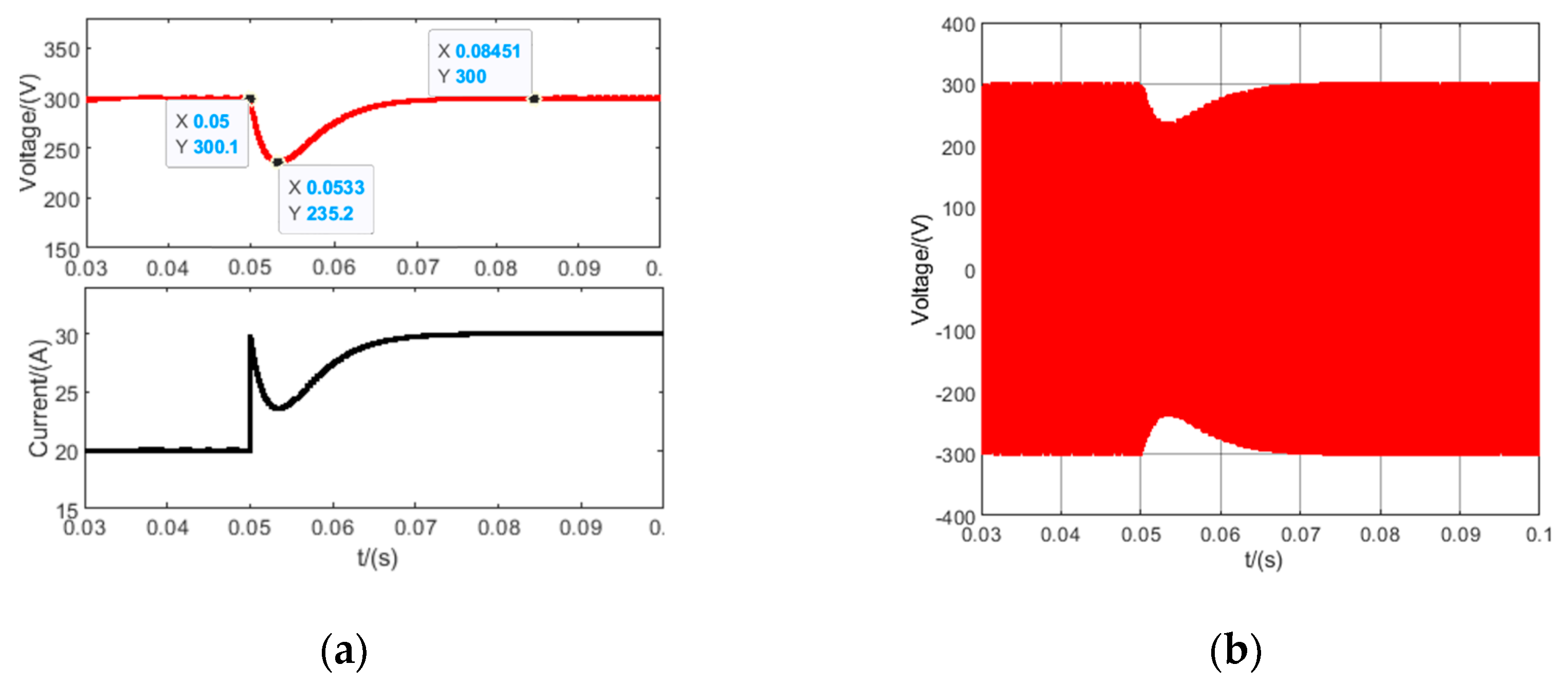
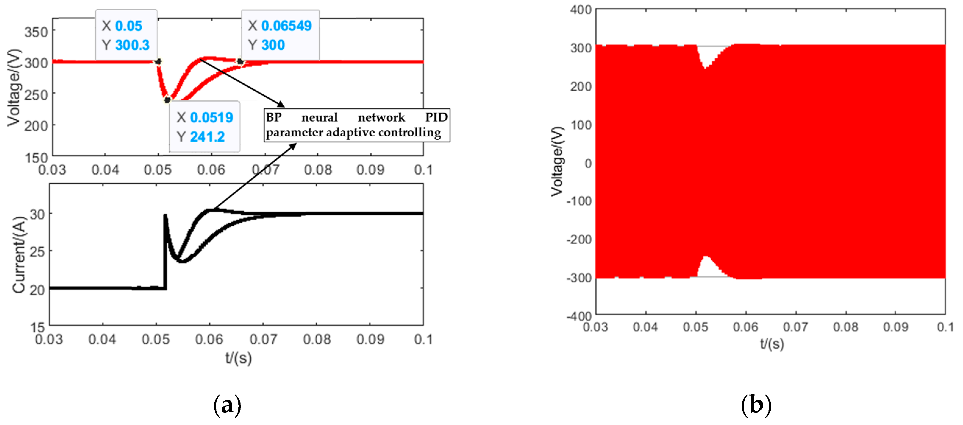
4.1. Simulation and Comparison with Traditional Incremental PID Controller

The construction of the controller and the implementation of the control algorithm were carried out in MATLAB Simulink. The input quantities returned to the neural network module included the system outputs y(k) and y(k − 1) at different time points, the system input r(k), the system output error e(k), e(k − 1), e(k − 2), the controller output u(k − 1), and the individual elements of the weight matrix. The controller’s output, u, represents the modulation signal for the phase-shift angle. The values of the learning rate η and the inertia coefficient α are set to 0.05 and 0.1, respectively. According to the previous analysis, the secondary-side control is mainly used, and the given of the system was set as the reference value of the control target. Control the secondary-side fully controlled rectifier bridge was controlled the load was changed from 15 Ω to 10 Ω at 0.08 s. The output constant voltage was taken as the control objective, and the voltage reference value was set to 300 V to obtain the simulation results. For the adjustment of the two sets of weights, the number of nodes in the implied layer was set to 8. The weight between the input layer and the hidden layer was defined as w_i, the weight between the hidden layer and the output layer was defined as w_o, and the input and output were both three nodes. Initial values were assigned to both matrices, and each set of weights was corrected by back-propagation of the error after the simulation was started, as shown in Figure 6a, and after a load change of 0.08 s, each weight was adjusted according to the error and stabilized again after about 0.007 s. The adjustment of each coefficient of the PID is shown in Figure 6b. It can be seen that, after the adaptive adjustment after the load change, the integral parameter k_i parameter has the largest change.

The traditional incremental PID controller was built and compared with the improved BP neural network PID parameter-adaptive control method. Figure 7a shows the output under incremental PID control. The voltage value decreases after the load change, the maximum overshoot is −64.9 V, and the output voltage recovers to 300 V after a perturbation of 0.035 s, which realizes the closed-loop control. Figure 7b shows the corresponding variation curve of the input AC voltage of the rectifier. It can be see in the output under adaptive control of the neural network parameters in Figure 8, that the overshoot under this control algorithm is reduced to −49 V, and the output voltage recovers to 300 V after 0.015 s of disturbance. Compared with traditional incremental PID, the overshoot of the system is reduced from −64.9 V to −49 V, and the adjustment time is shortened from 0.035 s to 0.015 s. The BP neural network PID parameter-adaptive control reduces overshoot by 25.5% and response time by 57.1%, verifying the advantages of this control algorithm.

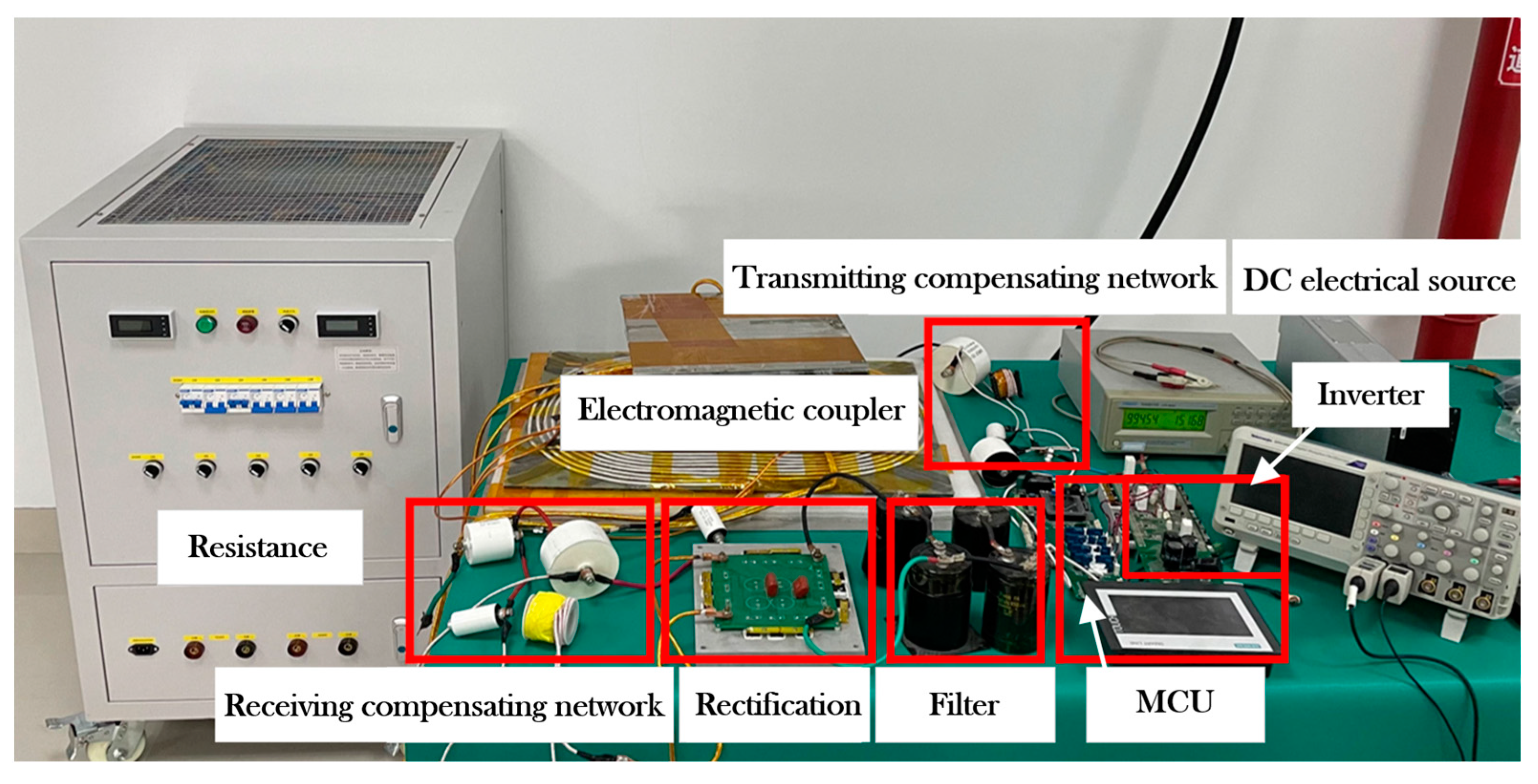
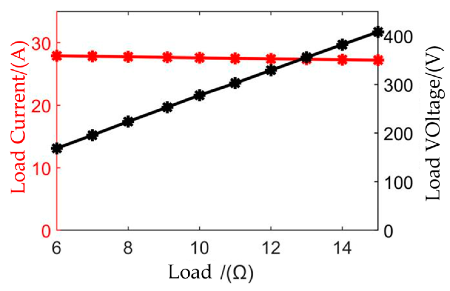
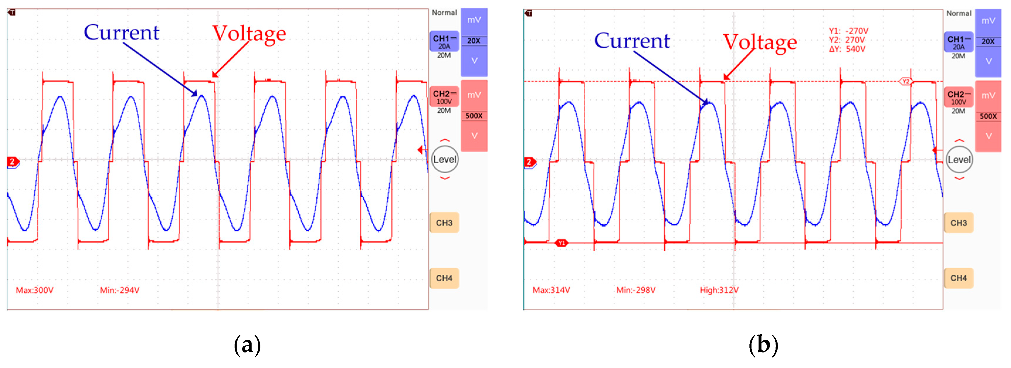
4.2. Experimentation

To demonstrate the rationality and effectiveness of the previous analysis, a dual LCC structure high-power electric vehicle wireless charging experimental platform was built for the experimental verification. The circuit parameters are shown in

Table 2. System parameters.

Parameter	Value	Parameter	Value
Lf1/(μH)	19.451	Lf2/(μH)	12.1
Cf1/(nF)	180.423	Cf2/(nF)	292.16
C1/(nF)	127.262	C2/(nF)	107.43
Lp/(μH)	47.20	Ls/(μH)	47.61
Udc/(V)	425	Req/(Ω)	6–15
Uref/(V)	270	f/(kHz)	85

. The system consists of a 20 kW DC charging module NXR75030 (Winline Technology, Shenzhen, China), high-frequency inverter, dual LCC compensation circuit, rectifier, filtering circuit, and a high-power adjustable load box. The control adopts a bilateral collaborative control method, and the communication between the primary and secondary sides is achieved through a 2.4 G module. In this system, 100 information transfers can be achieved within 1 s. The IMZ120R045M1 (Infineon, Munich, Germany) silicon carbide MOSFET is used, with a maximum withstand voltage of 1200 V, extremely low switching loss, and a wide gate-source voltage range. It is easy to drive and can perform synchronous rectification. The driving circuit adopts four ISO5852S gate drive chips. STM32F407 (STMicroelectronics, Geneva, Switzerland) is used as the control core, with 82 GPIO ports and a maximum CPU frequency of 168 MHz, meeting the system control requirements. Figure 9 shows the overall diagram of the high-power radio energy transmission system experimental platform, which is suitable for electric vehicles.

The dual LCC structure has the characteristic of constant current output, and the output current is not affected by load changes. Open-loop experiments on constant current output were conducted to verify this characteristic. The MOSFET of the secondary rectifier bridge was placed in a fully open state. The voltage and current values at the load end, and the load increases from 6 Ω to 15 Ω in steps of 1 Ω, were recorded. As shown in Figure 10, as the load increases, the load current remains basically unchanged, while the load voltage increases linearly with the load.

After verifying the output constant current characteristics of the double LCC structure with an open loop, a further closed-loop experiment was conducted to realize the rapid constant voltage control at both ends of the load by adjusting the rectification bridge of the auxiliary edge. The DC input voltage was set to 425 V, the set output voltage was 270 V, and the initial load was set to 10 Ω. Because the resistance box was used in the experiment, the load was adjusted and graded, i.e., the load was gradually adjusted to 10 Ω, 10.17 Ω, 10.53 Ω, 10.91 Ω, and 12 Ω. Figure 11a shows the voltage and current waveform of the two ends in the case of load mutation. With an increase in load, the current at the load end decreased accordingly, while the output voltage remained stable, and the actual voltage value was kept at 267 V, so that the set target value was reached in the presence of a sampling error. Figure 11b shows the overall waveform of the input end of the auxiliary side rectifier bridge. As the load resistance increases, the output voltage amplitude remains unchanged, and the output current amplitude gradually decreases.

The figure illustrates the AC voltage and current waveform of the input end of the rectifier bridge before and after the load change. At a load of 10 Ω, Figure 12a is the rectification bridge input waveform, when the voltage ring has taken effect, and the rectification bridge input voltage duty ratio is slightly below 50% due to the dead zone. When the load changes to 12 Ω, Figure 12b shows the input voltage and current waveform of the rectification bridge. After the load change, the controllable rectification becomes more effective, the input voltage duty ratio of the rectification bridge becomes significantly smaller, and the secondary closed-loop control of the output constant voltage is effectively realized.

5. Conclusions

This paper proposed a bilateral cooperative control strategy for an EV wireless power transfer system based on a BP neural network to realize closed-loop constant voltage control for the secondary rectifier circuit. This paper designed a control strategy based on the controller structure of a bidirectional energy wireless transmission system and selected a dual-phase-shift control method to achieve maximum power output according to the actual needs of the system. On this basis, in order to improve system stability and effectively achieve a fast response to disturbances, a PID parameter-adaptive controller based on a BP neural network was designed. Finally, a simulation and experimental verification compared the strategy with traditional control methods. The system achieved a control target with an output voltage constant at 267 V near the set value when the load changed. The control strategy has the advantages of shortening the response time and reducing overshoot. A constant pressure control experiment for the secondary rectifier bridge was also completed, showing an output power of up to 10.3 kW and a maximum efficiency of 92.96%, realizing closed-loop control with stable output.

References

1. Ma, M. Thoughts on the Development of Frontier Technologies in Electrical Engineering. J. Electr. Eng. Technol. 2021, 36, 4627–4636. [Google Scholar]
2. Yang, Q.; Zhang, X.; Zhang, P. Intelligent Wireless Power Transmission Cloud Network for Electric Vehicles. J. Electr. Eng. Technol. 2023, 38, 1–12. [Google Scholar] [CrossRef]
3. Husain, I.; Ozpineci, B.; Islam, M.S.; Gurpinar, E.; Su, G.J.; Yu, W.; Chowdhury, S.; Xue, L.; Rahman, D.; Sahu, R. Electric drive technology trends, challenges, and opportunities for future electric vehicles. Proc. IEEE 2021, 109, 1039–1059. [Google Scholar] [CrossRef]
4. Fan, X.; Mo, X.; Zhang, X. Research Status and Application of Wireless Power Transmission Technology. Proc. Chin. Soc. Electr. Eng. 2015, 35, 2584–2600. [Google Scholar]
5. Kang, Z.; He, S.; Li, P. Overview of Wireless Charging for New Energy Vehicles. Auto Ind. Res. 2019, 04, 48–53. [Google Scholar]
6. Diao, L.; Zhang, L.; Zeng, Y. Analysis of charging technology and application for new energy electric vehicles. China Electr. Equip. Ind. 2019, 10, 70–73. [Google Scholar]
7. Pang, B.; Deng, J.; Liu, P.; Wang, Z. Secondary-side power control method for double-side LCC compensation topology in wireless EV charger application. In Proceedings of the IECON 2017—43rd Annual Conference of the IEEE Industrial Electronics Society, Beijing, China, 29 October–1 November 2017; IEEE: Piscataway, NJ, USA, 2017. [Google Scholar]
8. Zou, S.; Onar, O.C.; Galigekere, V.; Pries, J.; Su, G.J.; Khaligh, A. Secondary Active Rectifier Control Scheme for a Wireless Power Transfer System with Double-Sided LCC Compensation Topology. In Proceedings of the IECON 2018—44th Annual Conference of the IEEE Industrial Electronics Society, Washington, DC, USA, 21–23 October 2018; IEEE: Piscataway, NJ, USA, 2018. [Google Scholar]
9. Nguyen, B.X.; Vilathgamuwa, D.M.; Foo, G.H.B.; Wang, P.; Ong, A.; Madawala, U.K.; Nguyen, T.D. An Efficiency Optimization Scheme for Bidirectional Inductive Power Transfer Systems. IEEE Trans. Power Electron. 2015, 30, 6310–6319. [Google Scholar] [CrossRef]
10. Zhang, B.; Gao, F.; Li, H.; Zhao, Y.; Tang, H.; Liu, X. Duty Cycle Control of Dual-side LCC Compensated Bidirectional Wireless Charging Systems. In Proceedings of the 2020 IEEE 9th International Power Electronics and Motion Control Conference (IPEMC2020-ECCE Asia), Nanjing, China, 29 November–2 December 2020; IEEE: Piscataway, NJ, USA, 2020. [Google Scholar]
11. Liu, F.; Chen, K.; Jiang, Y.; Zhao, Z. Research on the Overall Efficiency Optimization of the Bidirectional Wireless Power Transfer System. Trans. China Electrotech. Soc. 2019, 34, 891–901. [Google Scholar]
12. Zhao, S.; Li, Y.; Wu, D.; Mai, R. Current-Decomposition-Based Digital Phase Synchronization Method for BWPT System. IEEE Trans. Power Electron. 2021, 36, 12183–12188. [Google Scholar] [CrossRef]
13. Tavakoli, R.; Dede, E.M.; Chou, C.; Pantic, Z. Cost-Efficiency Optimization of Ground Assemblies for Dynamic Wireless Charging of Electric Vehicles. IEEE Trans. Transp. Electrif. 2022, 8, 734–751. [Google Scholar] [CrossRef]
14. Chen, K.; Pan, J.; Yang, Y.; Cheng, K.W.E. Stability Improvement and Overshoot Damping of SS-Compensated EV Wireless Charging Systems With User-End Buck Converters. IEEE Trans. Veh. Technol. 2022, 71, 8354–8366. [Google Scholar] [CrossRef]
15. Tavakoli, R.; Shabanian, T.; Dede, E.M.; Chou, C.; Pantic, Z. EV Misalignment Estimation in DWPT Systems Utilizing the Roadside Charging Pads. IEEE Trans. Transp. Electrif. 2021, 8, 752–766. [Google Scholar] [CrossRef]
16. Shi, K.; Tang, C.; Long, H.; Lv, X.; Wang, Z.; Li, X. Power Fluctuation Suppression Method for EV Dynamic Wireless Charging System Based on Integrated Magnetic Coupler. IEEE Trans. Power Electron. 2022, 37, 1118–1131. [Google Scholar] [CrossRef]
17. Qing, X.; Su, Y.; Hu, A.P.; Dai, X.; Liu, Z. Dual-Loop Control Method for CPT System Under Coupling Misalignments and Load Variations. IEEE J. Emerg. Sel. Top. Power Electron. 2022, 10, 4902–4912. [Google Scholar] [CrossRef]
18. Dai, X.; Li, X.; Li, Y.; Hu, A.P. Maximum efficiency tracking for wireless power transfer systems with dynamic coupling coefficient estimation. IEEE Trans. Power Electron. 2018, 33, 5005–5015. [Google Scholar] [CrossRef]
19. Wang, P.; Zuo, Z.; Sun, Y.; Li, X.; Fan, Y. Full-Duplex Simultaneous Wireless Power and Data Transfer System Based on Double-Sided LCC Topology. Trans. China Electrotech. Soc. 2021, 36, 4981–4991. [Google Scholar]
20. Bac, N.X.; Vilathgamuwa, D.M.; Madawala, U.K. A SiC-Based Matrix Converter Topology for Inductive Power Transfer System. IEEE Trans. Power Electron. 2014, 29, 4029–4038. [Google Scholar]
21. Hong, Y.; Cai, C. Self-Tuning Control Method for Wide-Area Wireless Power Supply with Multiple Transmitter Coils Efficient Coupling. Journal of Wuhan University (Engineering Edition), pp. 1–10. Available online: http://kns.cnki.net/kcms/detail/42.1675.T.20230530.1711.002.html (accessed on 6 November 2023).
22. Wang, Q.; Xia, L.; Han, J. Improved Particle Swarm Optimization of Linear Motor Fuzzy PID Control. J. Hefei Univ. Technol. (Nat. Sci. Ed.) 2022, 45, 458–463+474. [Google Scholar]
23. Killingsworth, N.; Krstic, M. PID Tuning Using Extremum Seeking. IEEE Control. Syst. Mag. 2006, 26, 70–79. [Google Scholar]
24. Zipser, D.; Andersen, R.A. A back-propagation programmed network that simulates response properties of a subset of posterior parietal neurons. Nature 1988, 331, 679–684. [Google Scholar] [CrossRef]
25. Lockery, S.R.; Wittenberg, G.; Kristan, W.B., Jr.; Cottrell, G.W. Function of identified interneurons in the leech elucidated using neural networks trained by back-propagation. Nature 1989, 10, 468–471. [Google Scholar] [CrossRef]
26. Hijmans, R.J.; van Etten, J. Raster: Geographic Analysis and Modeling with Raster Data. R Package Version 2.0-12. Available online: http://CRAN.R-project.org/package=raster (accessed on 12 January 2012).
Figure 1. Circuit of dual LCC topology.
Wevj 15 00026 g001
Figure 2. Equivalent circuit of dual LCC topology.
Wevj 15 00026 g002
Figure 3. TPS control mode voltage waveform diagram.
Wevj 15 00026 g003
Figure 4. Parameter-adaptive PID control structure based on BP neural network.
Wevj 15 00026 g004
Figure 5. Three-layer BP neural network structure.
Wevj 15 00026 g005
Figure 6. (a) Adjustment process of weight wi and wo; and (b) adjustment process of kp, ki and kd.
Wevj 15 00026 g006
Figure 7. Controlling results of incremental PID: (a) phase-shift angle and load voltage adjustment process; and (b) AC voltage waveform.
Wevj 15 00026 g007
Figure 8. Results of BP neural network PID parameter-adaptive control: (a) phase-shift angle and load voltage adjustment process; and (b) AC voltage waveform.
Wevj 15 00026 g008
Figure 9. Overall diagram of high wireless power transfer system experiment platform.
Wevj 15 00026 g009
Figure 10. Constant output current characteristic of dual LCC structure.
Wevj 15 00026 g010
Figure 11. Under resistance varying from 10 Ω to 12 Ω: (a) load voltage and current; and (b) rectifier input AC voltage and current.
Wevj 15 00026 g011
Figure 12. Under resistance with loads varying from 10 Ω to 12 Ω: (a) 10 Ω load; and (b) 12 Ω load.
Wevj 15 00026 g012