Lane Change Trajectory Planning Based on Quadratic Programming in Rainy Weather

Abstract

To enhance the safety and stability of lane change maneuvers for autonomous vehicles in adverse weather conditions, this paper proposes a quadratic programming−based trajectory planning algorithm for lane changing in rainy weather. Initially, in order to mitigate the risk of potential collisions on wet and slippery road surfaces, we incorporate the concept of road adhesion coefficients and delayed reaction time to refine the establishment of the minimum safety distance. This augmentation establishes constraints on lane change safety distances and delineates the boundaries of viable lane change domains within inclement weather contexts. Subsequently, adopting a hierarchical trajectory planning framework, we incorporate visibility cost functions and safety distance constraints during dynamic programming sampling to ensure the safety of vehicle operation. Furthermore, the vehicle lane change sideslip phenomenon is considered, and the optimal lane change trajectory is obtained based on the quadratic programming algorithm by introducing the maneuverability objective function. In conclusion, to verify the effectiveness of the algorithm, lateral linear quadratic regulator (LQR) and longitudinal double proportional−integral−derivative (DPID) controllers are designed for trajectory tracking. The results demonstrate the algorithm’s capability to produce continuous, stable, and collision−free trajectories. Moreover, the lateral acceleration varies within the range of ±1.5 m/s², the center of mass lateral deflection angle varies within the range of ±0.15°, and the yaw rate remains within the ±0.1°/s range.

1. Introduction

With the rapid development of autonomous driving technology, safety concerns are gradually garnering widespread attention. Within this trend, adverse weather conditions have gradually emerged as a prominent factor impacting road traffic safety [1]. Recent relevant studies have indicated [2] that up to 75% of annual traffic accidents occur on wet and slippery road surfaces. This has presented even more formidable challenges for autonomous vehicles. Particularly in rainy weather conditions, rapid lane change behavior is often liable to cause accidents such as side scraping and rear−end collisions [3]. Analyzing the causes of accidents, we found that rainfall leads to a decrease in the road surface adhesion coefficient, which affects the vehicle’s grip on wet and slippery road surfaces and has an impact on the vehicle’s stability, thus reducing the braking performance and extending the emergency braking distance; concurrently, rainfall reduces driver visibility, thereby affecting the driver’s field of vision for safe operation and increasing reaction times [4].

However, within the current research landscape, most of the studies within the crucial domain of lane change motion planning have not adequately addressed the impact of adverse weather conditions on motion planning. To mitigate uncertainties during autonomous vehicle operation and to enhance driving safety, it is imperative to incorporate the potential risks arising from environmental factors into the pivotal domain of motion planning [5].

Currently, the trajectory planning for autonomous vehicles is rooted in mobile robot path planning techniques. To adapt a multitude of autonomous navigation techniques to the domain of autonomous driving and to make the corresponding improvements, considerations are given to road network structures and traffic rule constraints [6]. According to the application methods of the planning techniques in autonomous driving, these methods can be roughly categorized into five classes: graph search methods, potential field methods, interpolation methods, sampling methods, and numerical optimization methods [7].

Among them, graph search−based planning algorithms describe the location of an object based on the grid it occupies by rasterizing or meshing the state space of the environment and deriving a route of movement based on the traversal of the state space [8]. However, related algorithms such as Dijkstra, A*, and D*, to name a few [9], plan paths that are not necessarily optimal and do not take into account road geometry constraints or poor trajectory smoothing. Based on potential field methods, the planning approach introduces the concept of potential fields. It abstracts the vehicle’s motion as the movement of a vector field, assigning attractive fields to safe areas for the vehicle and repulsive fields to obstacles. The vehicle’s future trajectory is planned by calculating the resultant force field it experiences [10]. However, these methods depend on accurately modeling the surrounding environment, which can lead to local optima. To compensate for this deficiency, Yang W [11] proposed an improved automatic obstacle avoidance method combining A* and artificial potential fields to solve the planning and tracking problems of autonomous vehicles in road environments.

Because of the limitations of the potential field method, researchers have also introduced interpolation−based planning algorithms [12]. This method utilizes geometric curves as its foundation, interpolating intermediate nodes based on known starting and ending points to generate smooth trajectories. This results in generated lane change trajectories possessing continuous curvature and ensuring that the vehicle reaches its destination at the desired speed and posture [13]. In their study, Zeng et al. employed third−order B−spline curves for lane change trajectory planning. 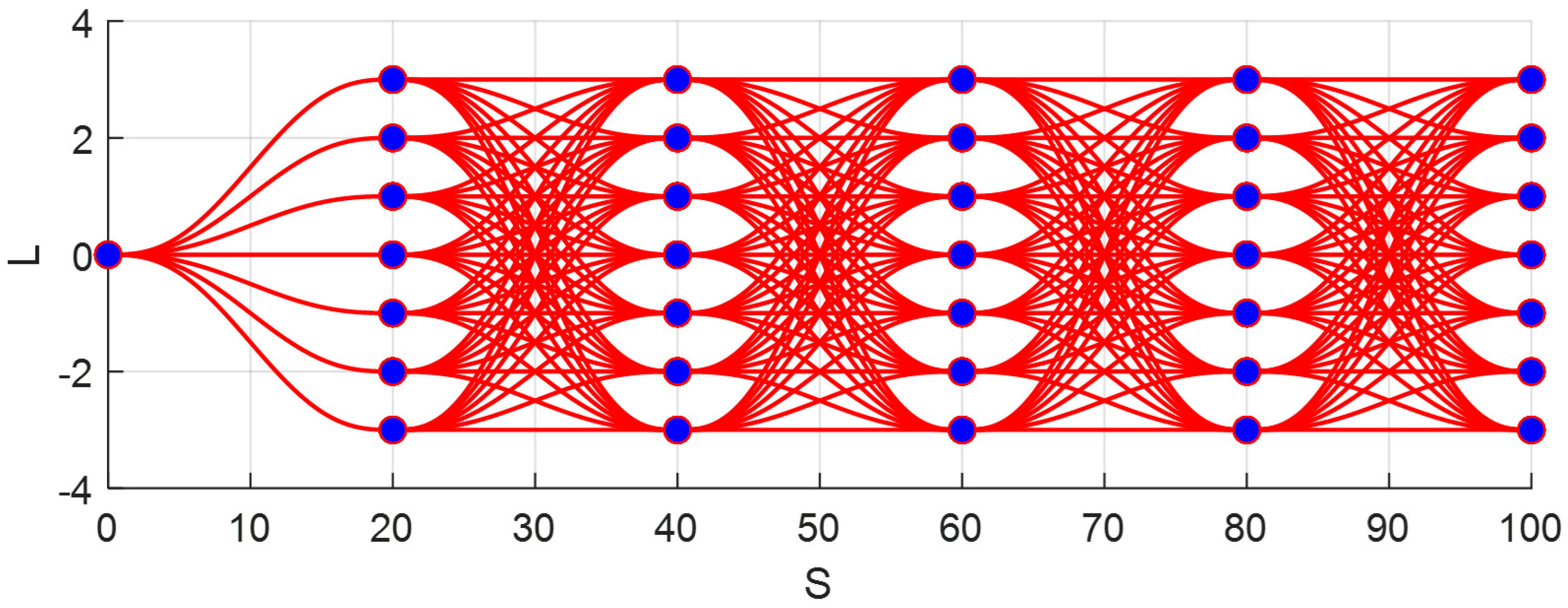By simultaneously considering the constraints of the host vehicle, they achieved the generation of ideal trajectories [14]. However, this approach requires the appropriate interpolation density, as interpolation which is too low can impact accuracy and lead to local errors, while excessively high interpolation can affect real−time computation. Currently, methods capable of performing motion planning tasks on structured roads can be classified into two categories: sampling−based methods and numerical optimization−based methods [15]. Sampling−based methods offer an intuitive way to express complex abstract spaces and find globally optimal solutions in discretized intricate road environments [16]. Conversely, numerical optimization−based methods capitalize on precise modeling, rapidly converging to minimal values through numerical optimization to identify local optimal solutions [17]. Consequently, the motion planning solutions of most advanced autonomous vehicles leverage the strengths of these two methods, establishing a hierarchical framework involving sampling followed by optimization [18].

B. Li et al. proposed a layered trajectory planning framework that combines sampling and numerical optimization. The upper- −level planner samples rough trajectories, while the lower−level planner refines trajectories using numerical optimization methods [19]. This approach formulates the trajectory generation problem as an optimal control problem, employing numerical optimization to solve multi−objective functions and obtain trajectories that are continuous, comfortable, and collision−free, while adhering to various constraints [20]. Furthermore, to enhance the operational limits of autonomous vehicles, Chen et al. devised a hierarchical dynamic drifting controller (HDDC) which, through the implementation of drifting and cornering maneuvers, achieves trajectory tracking control within and beyond the confines of stability limits [21]. Additionally, Zhang et al. introduced a synchronous planning and control scheme that obviates the necessity for explicit trajectory planning and instead determines control inputs based solely on relevant control objectives and safety constraints [22]. In a different vein, Chen et al. addressed FWIC−EV chassis control strategy, proposing a comprehensive control strategy predicated on slip control. Specifically tailored for regular driving conditions, this strategy aims to minimize tire slip power loss and bolster the efficacy of the anti−slip braking system [23]. Considering the impact of environmental factors, Yu et al. [24] introduced an active perception algorithm that explores the surrounding environment through a loop between perception and trajectory generation. This aims to reduce uncertainties and risks in the environment [25]. Wang et al. incorporated visibility prediction into trajectory planning, introducing a risk metric based on predicted visibility to penalize trajectories with high speed and low visibility [26]. Li Z et al. addressed lane change scenarios on wet and slippery road surfaces, introducing a longitudinal safety model to assess safety before and after lane changes and to mitigate issues related to lateral slip through tire slip angle evaluation [27]. The aforementioned references primarily focus on enhancing vehicle stability from the perspective of vehicle tracking control. Alternatively, within a phase of trajectory planning, the emphasis is solely placed on ensuring the safety of vehicle operation on wet and slippery road surfaces, thereby resulting in an excessively cautious generation of the target trajectory.

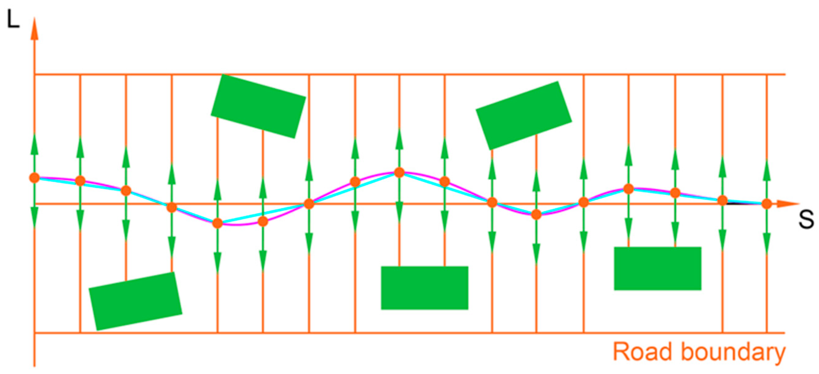
Therefore, the primary focus of this study is to generate safer and more stable lane change trajectories on low−adhesion wet and slippery road surfaces. Firstly, based on the improved minimum safe distance, this paper introduces safety distance constraints for rainy weather scenarios and the boundaries of lane change feasible regions. Secondly, within the framework of a layered trajectory planning approach, a visibility cost function and improved safety distance constraints are incorporated into the dynamic planning process. Finally, a quadratic programming algorithm is employed to introduce a vehicle stability objective function, resulting in optimal lane change trajectories that ensure continuity, stability, and collision−free operation. The specific tasks undertaken in the remainder of this paper are as follows:

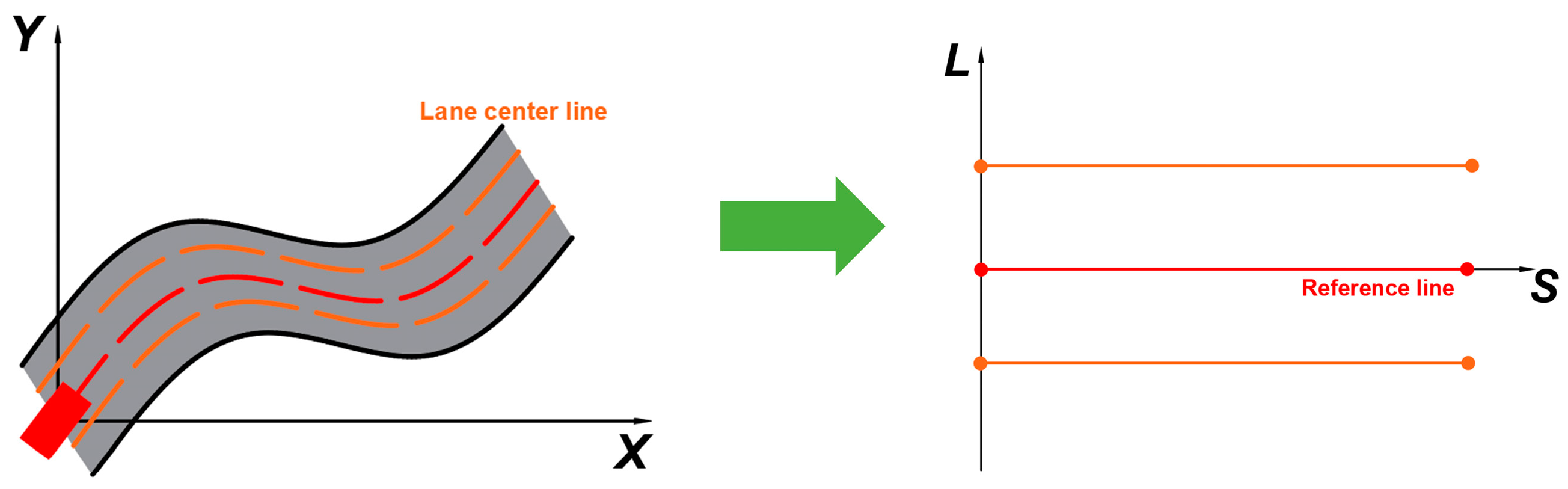
Section 2 quantitatively analyzes the impact of rainfall on lane change behavior, proposing safety distance and lane change feasible region boundaries for rainy weather scenarios. Within the sampling−based, followed by the optimization−based, layered trajectory framework, Section 3 introduces the visibility cost function and the vehicle stability objective function. Section 4 presents the design of the lateral LQR controller and the longitudinal DPID controller to verify the effectiveness of the algorithm. Section 5 presents the simulation results and analysis. Section 6 summarizes the contributions and limitations of this paper, discussing future research directions and challenges.

2. Quantitative Analysis of Rainy Weather Impact on Lane Change Maneuvers

Rainfall has several significant impacts on vehicle operation: firstly, it reduces the coefficient of friction on road surfaces, leading to diminished braking performance and extended emergency braking distances. Secondly, rain also decreases driver visibility, affecting their field of vision for safe driving and increasing reaction times [20]. Therefore, this paper aims to introduce the attachment coefficient and reaction delay time based on the minimum safe distance by analyzing the characteristics of lane change behavior in rainy weather scenarios. At the same time, the concepts of safe distance for lane changing and following distance in rainy weather scenarios are proposed to establish more accurate boundary conditions for the feasible domain of lane changing in rainy weather. In order to consider driving safety and handling stability, this paper introduces the visibility cost function and the handling stability objective function in the process of dynamic and quadratic planning. The overall research architecture is shown in Figure 1.

2.1. Coefficient of Friction

The coefficient of friction is influenced by various factors, including road surface materials, tire pressure, vehicle speed, and others [7]. J. Tian et al. quantitatively analyzed the interrelationship between the coefficient of friction [10], vehicle speed, and water film thickness by exploring the relationship between rainfall intensity and water film thickness. The relationship between rainfall intensity and water film thickness can be expressed as follows:

$$h=0.1258\times l^{0.6715}\times i^{-0.3147}\times d^{0.7786}\times T{D}^{0.7261}(R^2=0.93)$$

(1)

where h represents water film thickness (mm), l denotes slope length (m), i stands for slope gradient (%), d represents rainfall intensity, and TD signifies road construction depth (mm). According to the findings in reference [7], which reveal the interrelationship between the coefficient of friction, vehicle speed, and water film thickness, we can deduce the relationship expression for the coefficient of friction under varying rainfall conditions:

$$\phi =0.6603-0.0037v-0.0057h$$

(2)

where φ represents the coefficient of friction, and v stands for vehicle speed (m/s). Due to tire wear requiring deceleration correction, in conjunction with Equations (1) and (2) [8] the expression for rainy weather braking deceleration [8] is:

$$a_f=a_r=\epsilon \times \phi \times g$$

(3)

where a_f and a_r are the front and rear wheel braking deceleration; ε is the correction factor, generally taking the value of 0.9; g is the acceleration of gravity (9.8 m/s²).

2.2. Delayed Reaction Time

In rainy conditions, an increase in rainfall intensity leads to reduced visibility, subsequently affecting the driver’s ability to react while driving and prolonging reaction times [20]. Therefore, we define driving delayed reaction time as the time interval between the occurrence of a certain unexpected situation or emergency event and the actual initiation of the corresponding driving actions [14]. The rainy weather driving delayed reaction time can be calculated as follows:

$$t_f=\frac{1}{v_0}(2S_d-S_f)-\frac{v_0}{2a_f}-t_r$$

(4)

Here, t_f represents the delayed reaction time, S_d is the critical value of safe visual distance (m), S_f stands for rainy weather visibility (m), and t_r is the normal reaction time, v₀ denotes the initial vehicle speed, with a value of 1 s [19].

According to the research results [28], it is evident that with an increase in rainfall intensity, visibility gradually decreases. For specific details, please refer to Figure 2. By utilizing the critical value of safe visual distance provided in reference [29] and applying Equation (4) for calculation, we can unveil the interrelationship between delayed reaction time and visibility under different rainfall intensities [30]. This relationship is depicted in Figure 3.

2.3. Lane Change Feasible Region in Rainy Conditions

The lane change feasible region is defined as the spatial area where a vehicle can complete a safe and obstacle−free lane change operation under ideal driving conditions [22]. Typically, determining this range is associated with various factors, including vehicle kinematic constraints, traffic flow, and the surrounding vehicle environment [8]. However, performing lane changes under adverse weather conditions requires special attention to factors such as wet road surfaces, reduced adhesion, and decreased visibility. Hence, it is imperative to establish safer and more accurate boundaries for the lane change feasible region. The spatial extent of the lane change feasible region encompasses the host vehicle’s current lane and the target lane, as illustrated in Figure 4.

In this subsection, we introduce the concept of following at a safe distance and lane changing at a safe distance in rainy weather scenarios to establish the boundary conditions for the rainy weather lane change feasible region. By thoroughly considering adverse environmental factors, the aim is to ensure the safety and effectiveness of lane change operations under unfavorable weather conditions.

2.3.1. Boundary Conditions for the Current Lane Feasible Region

When the host vehicle intends to execute a lane change within its current lane under rainy conditions, it maintains a specific following distance from the preceding vehicle. If the host vehicle’s speed is lower than that of the leading vehicle, the gap between them gradually increases with time. Conversely, when the host vehicle’s speed exceeds that of the leading vehicle, the gap diminishes progressively. If this distance becomes smaller than the minimum safe following distance for rainy conditions, any sudden event could lead to an inevitable collision between the two vehicles. The establishment of this safety gap is particularly vital on wet and slippery road surfaces in rainy weather. It ensures ample time and distance between vehicles for drivers to respond to unforeseen situations, thereby mitigating collision risks and ensuring safe driving. Refer to Figure 5 for a visual depiction.

In rainy conditions, when accounting for the effects of both delayed reaction time and the coefficient of friction, the distance covered by the host vehicle during steady−speed travel is formulated as:

$$L_f=v_0(t_r+t_f+t_{dd})$$

(5)

Here, v₀ denotes the initial vehicle speed; t_r is the normal reaction time; and t_dd signifies driving delay time. As delineated in reference [13], the braking process is divided into phases, where during the initial increase in braking, the distance covered is denoted as L_di, and during the continuous braking phase, the distance is L_c. The sum of the distances for each phase constitutes the total braking distance, denoted as L_f [26].

The total brake application time is denoted as t_d, comprising brake delay time t_dd and brake duration t_di (t_d = t_dd + t_di); typically, t_dd is set at 0.15 s and t_di at 0.1 s [15]. Following the lane change, vehicle A maintains a lower trailing speed. Upon the initiation of braking by vehicle A, vehicle B also engages in braking, with L_l as the braking distance, where L represents the distance maintained between the two vehicles when at a stop, which is usually set as L = 2 m [18]. Thus, the following safe distance under rainy conditions is proposed as:

$$\min (S_1)=L_f-L_l+L$$

(6)

As shown in Figure 4, the potential collision point of the host vehicle in the current lane is P1, and the coordinates of the host vehicle are expressed as Formula (7), based on the dimensional parameters of the vehicle and the kinematics [25]:

$$\left\{\begin{array}{c}{x}_{p1}\left(t\right)={\displaystyle \int {}_{t_m}^{t_{p1}}{v}_A\left(t\right)\cos \left[{\theta }_A\left(t\right)\right]}dt=D_1+{\displaystyle \int {}_{t_m}^{t_{p1}}{v}_F\left(t\right)}dt\\ y_{p1}\left(t\right)={\displaystyle \int {}_{t_m}^{t_{p1}}{v}_A\left(t\right)\sin \left[{\theta }_A\left(t\right)\right]}dt=b\end{array}\right.$$

(7)

where x_p1 and y_p1 denote the vehicle coordinate values on the X−axis and Y−axis, t_m is the lane change start time, and t_p1 denotes the time when the vehicle is at the collision point p₁.v_A is the speed of the host vehicle, θ_A is the vehicle yaw angle, D₁ is the longitudinal distance between the host vehicle A and the vehicle F in front of it, and b is the lateral distance driven by the host vehicle. v_F(t) is denoted as the speed of vehicle F. Therefore, the longitudinal distance OP₁ of the host vehicle should satisfy the minimum safe following distance in rainy weather, and the boundary conditions for the current lane in rainy scenarios are proposed as follows:

$$O{P}_1>\min \left(S_1\right)=L_f-L_l+L$$

(8)

2.3.2. Boundary Conditions for the Feasible Region of the Target Lane

Subsequent to the leading vehicle’s entry into the target lane, if the trailing vehicle’s speed surpasses that of the leading vehicle, the distance between the two vehicles will gradually diminish. Failure to maintain an adequate safety interval during this progression will inevitably lead to a collision between the leading vehicle and the following vehicle in the rear of the target lane. Therefore, establishing a secure clearance during a lane change becomes particularly critical in rainy conditions. It is vital to ensure that on wet and low−adhesion road surfaces there exists sufficient temporal and spatial room between vehicles to prevent collisions, as depicted in Figure 6. Assuming that leading vehicle A executes a lane change from time t₀ to time te, with a collision occurring at time t_c, the process analysis is outlined as follows:

$$S_0+L_A+S_A\ge S_B$$

(9)

where S₀ represents the initial vehicle separation distance, while the length of vehicle A is denoted as L_A. The distance covered by vehicle A from t₀ to t_c is represented by S_A, and the corresponding distance for vehicle B within the same time interval is denoted as S_B. If v_A < v_B, a collision between the vehicles will occur within the time t_c. To avoid such a collision, it is necessary to fulfill the condition stated in Equation (9). Conversely, if v_A > v_B, the target vehicle A will move away from vehicle B. In this situation, a certain safe distance for S₀ must be maintained to prevent the trailing vehicle from being unable to avoid a collision through emergency braking.

$$S_0\ge \left\{\begin{array}{c}(v_B-v_A)(t_c+t_f)v_A\le v_B\\ \frac{v_B^2}{2a_f}+v_B{t}_f{v}_A\ge v_B\end{array}\right.$$

(10)

where v_A, v_B are the speeds of vehicle A and vehicle B; t_c is the collision time, and the minimum safe distance for the rainy weather lane change process is proposed [18]:

$$\min (S_0)=\left\{\begin{array}{c}(v_B-v_A)(t_c+t_f)-L_A{v}_A\le v_B\\ \frac{v_B^2}{2a_f}+v_B{t}_f{v}_A\ge v_B\end{array}\right.$$

(11)

Let the collision point of the host vehicle in the target lane be P₂, as shown in Figure 4; similarly, its coordinates (x_p2, y_p2) can be expressed as:

$$\left\{\begin{array}{c}{x}_{p2}\left(t\right)={\displaystyle \int {}_{t_m}^{t_{p2}}{v}_A\left(t\right)\cos \left[{\theta }_A\left(t\right)\right]}dt={\displaystyle \int {}_{t_m}^{t_{p2}}{v}_R\left(t\right)}dt-D_2\\ y_{p2}\left(t\right)={\displaystyle \int {}_{t_m}^{t_{p2}}{v}_A\left(t\right)\sin \left[{\theta }_A\left(t\right)\right]}dt=w\end{array}\right.$$

(12)

where x_p2 and y_p2 denote the vehicle coordinate values on the X-axis and Y-axis, t_m is the lane change start time, t_p2 denotes the time when the vehicle is at the collision point p₂, V_A is the velocity of the host vehicle, θ_A is the vehicle yaw angle, v_R(t) is denoted as the speed of the rear vehicle B, D₂ is the longitudinal distance between the host vehicle A and the rear vehicle B, and W is the lateral distance driven by the host vehicle. Therefore, the longitudinal distance OP₂ from the host vehicle should satisfy the minimum lane change safety distance constraint in rainy weather, and the proposed lane change boundary condition for the target lane in a rainy weather scenario is:

$$O{P}_2>\min \left(S_0\right)=\left\{\begin{array}{c}\left(v_B-v_A\right)\left(t_c+t_f\right)-L_A{v}_A<v_B\\ \frac{v_B^2}{2a_f}+v_B{t}_f{v}_A\ge v_B\end{array}\right.$$

(13)

The coordinates of the potential collision points, P₁ and P₂, can be determined based on Equations (7) and (12). The constraints that P₁ and P₂ need to satisfy can be derived from Equations (8) and (13). Consequently, the feasible region for rainy day lane changing can be ascertained, as illustrated in Figure 4. The trajectories of OP₁ and OP₂ serve as boundary constraints, and the spatial region between OP₁ and OP₂ constitutes the viable rainy day lane change domain.

3. Lane Change Trajectory Planning

3.1. Dynamic Programming

3.1.1. Discrete Space Based on Rainy Day Lane Change Feasible Region

Considering the complexity of the trajectory search and the real−time requirements, we opted for the adoption of the Frenet coordinate system for computational convenience. The Frenet coordinate system employs the lane centerline as its reference, as illustrated in Figure 7. Through coordinate transformations between the Frenet and Cartesian coordinate systems, the trajectory search problem in roads with changing curvatures is simplified. It is transformed into a search for lateral offset L based on the reference axis S in the orthogonal space.

First, the extent of the search space is defined based on the rainy weather permutation feasible domain. Then, the longitudinal lengths and lateral offsets of the sampling points are defined to discretize the search space into a grid, as shown in Figure 8. The sampling points are generated using the following rules:

$$S=i\times \Delta s$$

(14)

$$L=j\times \Delta l$$

(15)

where N_ij denotes the vertices, i and j denote the row and column numbers, Δs denotes the S−direction unit spacing, and offset Δl is the sampling lateral offset.

We define the collection of sampling points, N_ij, with identical longitudinal distances as layer_i, and employ it to construct the search space for generating preliminary lane change trajectories. This search space encompasses a series of contiguous trajectory clusters, serving as potential lane change candidates. Through dynamic programming computations, we identify sampling points that fulfill the minimum cost criterion. Subsequently, accounting for the vehicle’s smooth operation, the first and second derivatives of the trajectory are continuous and smooth. Therefore, we employ quintic polynomials to connect adjacent sampling points, producing rough lane change trajectory candidates. Ultimately, we formulate a cost function to assess the quality of these trajectory candidates.

$$\begin{array}{l}x(t)=a_0{t}^5+a_1{t}^4+a_2{t}^3+a_3{t}^4+a_4{t}^5+a_5\\ y(t)=b_0{t}^5+b_1{t}^4+b_2{t}^3+b_3{t}^4+b_4{t}^5+b_5\end{array}$$

(16)

where lon = [a₀, a₁, a₂, a₃, a₄, a₅] is the longitudinal trajectory function coefficients, and lat = [b₀, b₁, b₂, b₃, b₄, b₅] is the lateral trajectory function coefficients; the rough trajectory of the lane change can be obtained as shown in Figure 9. It is represented in the Frenet coordinate system, as shown in Figure 10.

3.1.2. Cost Function

This subsection focuses primarily on elucidating the process of generating lane change trajectories tailored for environments characterized by reduced visibility and diminished road surface friction. We employ a cost function to systematically evaluate trajectory candidates with the aim of selecting the optimal driving behavior. Drawing from the content of reference [26], the cost function typically encompasses components related to the lane centerline and those associated with avoiding collisions with obstacles.

In this subsection, we account for the impact of rain on the driver’s visual field for safe driving, introducing a visibility−based cost function. Additionally, we enhance the constraint conditions of the collision avoidance cost function based on rainy day safety distances. We aggregate the aforementioned cost function components through weighted summation, thereby defining the cost function f_DP. Herein, w_vis, w_obs, and w_ref, respectively, represent the corresponding weight coefficients for the cost terms.

$$f_{DP}={\omega }_{vis}{J}_{vis}+{\omega }_{obs}{J}_{obs}+{\omega }_{ref}{J}_{ref}$$

(17)

$$J_{vis}=k_1{e}^{-{\left(S_n-S_f\right)}^2}$$

(18)

In this context, S_n represents the sampling points, S_f denotes the visibility (m) during rainy weather conditions, and k₁ stands for the proportional coefficient. Under rainy conditions, due to the decrease in visibility, it becomes necessary to reduce the scope of the trajectory planning to enhance driving safety. Additionally, when the range of sampling points exceeds the current visibility limitations, the visibility cost function J_vis is introduced to impose penalties. Similarly, during favorable visibility conditions, it becomes feasible to expand the trajectory planning scope, thereby enabling the dynamic adjustment of trajectory ranges. The parameter values are detailed in

Table 1. Simulation parameters.

Parameters	Value
Vehicle weight, m	2.02 t
Sampling time, t	0.05 s
Wheelbase, L	2.947 m
wobs, wref, wacc, wjerk, wsmo	300, 100, 20, 80, 60
k1, k2, k3, k4, k5, k6, k7, k8	40, 20, 15, 30, 20, 20, 10, 5
Moment of inertia, Iz	4.095 t/rad
Distance constant dn, dc	4, 2
Sampling lateral distance, Δl	1 m
Longitudinal sampling distance, Δs	10 m
Front wheel cornering stiffness, cf	175.016 kN/rad
Rear wheel cornering stiffness, cr	130.634 kN/rad
Distance from center of mass to rear axis, b	1.682 m
Distance from center of mass to front axle, a	1.265 m

.

$$J_{obs}\left\{\begin{array}{c}0\\ J_{nudge}=k_1\times e^{-\left(d-d_c\right)}\\ J_{collision}=\infty \end{array}\right.\begin{array}{c}d>d_n\\ d_c\le d\le d_n\\ d<d_c\end{array}$$

(19)

$$dc=k_2\min \left(S_0\right)+k_3\min \left(S_1\right)$$

(20)

The collision avoidance cost function, denoted as J_obs, imposes penalties based on the distance between the ego vehicle and the obstacles. With the slippery road conditions and the reduced coefficient of friction due to rainy weather, the braking performance deteriorates, leading to an increase in braking distance. Therefore, we introduce an exponential function, as defined in Equations (6) and (11) to establish a safety distance constraint and to apply penalties to sampling points. Here, d represents the distance between the ego vehicle and the obstacles; k₁, k₂, k₃, and k₄ are proportionality coefficients, and d_n signifies the rainy weather nudge safety distance. When d_c ≤ d ≤ d_n, the exponential function J_nudge is introduced, representing a sharp increase in collision cost as the distance decreases. When d becomes smaller than the minimum collision distance d_c, the cost function J_collision reaches a maximum value. The parameter values are detailed in Table 1.

$$J_{ref}={\displaystyle \int {\left(f_{ref}\left(s\right)-g_l\left(s\right)\right)}^2}ds$$

(21)

The lane reference line cost function, denoted as J_ref, is designed to encourage the vehicle to travel along the centerline of the lane. Here, f_ref represents the lane centerline, g_l signifies a sampling point, and J_ref imposes penalties on sampling points g_l that deviate significantly from the lane centerline. According to the cost function, a traversal of the sampling points is performed to search for the sampling point with the minimum cost. Subsequently, by connecting the sampling points using a fifth−degree polynomial, a preliminary lane change trajectory is obtained, as illustrated in Figure 11.

3.2. Quadratic Programming

In this subsection, the precise trajectory optimization problem undergoes a transformation into an optimal control problem (OCP). This entails the formulation of an objective function that necessitates construction and subsequent solution, while adhering to a spectrum of constraints [22]. To accommodate considerations of passenger comfort, it is customary to construct acceleration and jerk objective functions, coupled with the design of a smoothness objective function, all aimed at ensuring a comfortable driving experience [28]. Nevertheless, within the context of rainy weather scenarios, the demands placed on trajectory maneuverability become notably stringent due to the potential occurrence of sideslip phenomena during lane change maneuvers. Consequently, we introduce a maneuver stability objective function and improve the dynamic constraints to effectively address this challenge.

The solution of the precise trajectory needs to be based on the rough trajectory, and we use the derived rough trajectory as a guideline and also as a guess value of the obstacle nudge distance to provide the initial value for the solution of the precise trajectory, as shown in Figure 12. In this paper, the objective function of the exact trajectory is optimally solved based on the method of quadratic programming. Its standard form is expressed as:

$$\begin{array}{c}\mathrm{minimize}\frac{1}{2}{X}^{T}HX+f^{T}X\\ st.Ax\le b\end{array}$$

(22)

In the equation, x represents the control variables, H denotes the Hessian matrix, and f is the gradient vector. The hard constraints encompass the inequality constraints that must be adhered to during the lane change process. The objective function is intricately tied to the trajectory’s smoothness and acceleration variation. To satisfy the criteria for comfort, stability, and trajectory smoothness during rainy weather lane changes, the objective function is defined as follows:

$$f_{QP}=\underset{i}{\overset{N_m}{\Sigma }}{\omega }_{sta}{J}_{stability}+{\omega }_{acc}{J}_{acc}+{\omega }_{jerk}{J}_{jerk}+{\omega }_{smo}{J}_{smooth}$$

(23)

where N_m signifies the total number of trajectory nodes in the optimization stage, ω_sta represents the weight for the stability cost, ω_acc denotes the weight for the acceleration cost, ω_jerk stands for the weight for the jerk cost, and ω_smo indicates the weight for the smoothness cost.

$$J_{stability}=k_4{e}^{-{(a_l-a_{ldes})}^2}+k_5{e}^{-{(\phi -{\phi }_{des})}^2}$$

(24)

The stability objective function, denoted as J_stability, is defined using parameters representing lateral acceleration and yaw angle, which characterize stability. Here, φ represents the yaw angle; φ_des signifies the desired minimum yaw angle; and a_l and a_ldes, respectively, denote lateral acceleration and desired minimum lateral acceleration along the l direction, while k₄ and k₅ are proportionality coefficients. By imposing penalties on the trajectory points with significant deviations in lateral acceleration and yaw angle, manipulation stability and passenger comfort are improved.

$$a_{s,i}=\frac{s_{i+1}-2s_i+s_{i-1}}{\Delta t^2}$$

(25)

$$a_{l,i}=\frac{l_{i+1}-2l_i+l_{i-1}}{\Delta t^2}$$

(26)

$$J_{acc}=a_{s,i}^2+a_{l,i}^2$$

(27)

where a_s,i and a_l,i denote the acceleration along the s and l directions; this penalty function makes the curvature and longitudinal acceleration of the exact trajectory relatively flat. J_jerk is denoted as the rate of change of the acceleration and is defined as:

$$j_{s,i}=\frac{s_{i+2}-3s_{i+1}+3s_i-s_{i-1}}{\Delta t^3}$$

(28)

$$j_{l,i}=\frac{l_{i+2}-3l_{i+1}+3l_i-l_{i-1}}{\Delta t^3}$$

(29)

$$J_{jerk}=j_{s,i}^2+j_{l,i}^2$$

(30)

To ensure the smoothness of driving, penalties are imposed for abrupt changes in acceleration. Here, j_s,i and j_l,i, respectively, denote the rates of acceleration variation along the s direction and l direction.

$$J_{smooth}=k_6{{\displaystyle \int \left(f^{\prime }\left(s\right)\right)}}^{2}ds+k_7{{\displaystyle \int \left(f^{″}\left(s\right)\right)}}^{2}ds+k_8{{\displaystyle \int \left(f^{‴}\left(s\right)\right)}}^{2}ds$$

(31)

The smoothing objective function is denoted as J_smooth, which introduces penalties for trajectories with higher curvature to reduce the degree of bending. Here, f′(s) represents heading error, f″(s) is related to curvature, and the derivative of curvature, denoted as f‴(s), ensures minimal variation in trajectory curvature. The coefficients k₆, k₇, and k₈ are proportionality factors. The parameter values are detailed in Table 1.

Precise trajectory planning not only drives the minimum convergence point of the objective function but also adheres to vehicle dynamic constraints and environmental limitations. Considering the influence of wet and slippery road conditions and low adherence rates, the vehicle dynamic constraints are modified by incorporating Formula (2). This modification ensures that acceleration remains within the physical limits of the vehicle. Environmental constraints are often formulated using the circular disk model, as detailed in the reference [26].

$$a_{s,i}^2+a_{l,i}^2\le {\left(\phi a_{max}\right)}^2$$

(32)

where a_s,_i is the longitudinal acceleration, a_l,i is the lateral acceleration, and a_max is the maximum acceleration.

4. Trajectory Tracking Control

Driving in rainy weather is frequently affected by factors such as slippery roads and reduced traction; this makes lateral stability and longitudinal speed and position control of the vehicle critical. Therefore, in this paper, the lateral LQR controller and the longitudinal DPID controller are used to implement the trajectory tracking control [12], although the parameter settings of these two controllers are complex and computationally expensive. However, they have better stability and can reduce the risk of sideslip and loss of control. In addition, they are adaptable and robust in unstable environments. For trajectory tracking control, the focus is on the lateral motion of the vehicle. In order to simplify the calculation, a two−degrees−of−freedom vehicle dynamics model is used in this paper [15].

$$\left\{\begin{array}{l}m{a}_y=F_{yf}+F_{yr}\\ I_z\stackrel{·}{\omega }=l_f{F}_{yf}-l_r{F}_{yr}\end{array}\right.$$

(33)

$$\left\{\begin{array}{l}\stackrel{·}{v_y}=-\left(v_x+\frac{c_f{l}_f-c_r{l}_r}{m{v}_x}\right)\omega -\frac{c_f+c_r}{m{v}_x}{v}_y+\frac{c_f}{m}{\delta }_f\\ \stackrel{·}{\omega }=-\left(\frac{c_f{l}_f^2+c_r{l}_r^2}{I_z{v}_x}\right)\omega -\frac{c_f{l}_f-c_r{l}_r}{I_z{v}_x}{v}_y+\frac{c_f{l}_f}{I_z}{\delta }_f\end{array}\right.$$

(34)

where a_y is the acceleration along the body coordinate y direction at the center of mass of the vehicle; m is the mass of the vehicle; F_yf and F_yr are the combined lateral forces on the front and rear axle tires, respectively; I_z is the rotational moment of inertia of the vehicle around the z-axis of the center of mass; ω is the yaw rate of the vehicle; l_r and l_f are the distances from the vehicle’s center of mass to the front and rear axles of the vehicle; c_f and c_r are the lateral deflection stiffnesses of the tires on the front and rear axles of the vehicle, respectively; and δ_f is the front wheel angle.

Lateral and heading errors are mainly considered when the vehicle performs tracking to control the reference trajectory [21]. The error state space equation is expressed as:

$$\stackrel{·}{X}=AX+BU$$

(35)

$$A=\left[\begin{array}{cccc}0& 1& 0& 0\\ 0& -\frac{c_f+c_r}{m{v}_x}& \frac{c_f+c_r}{m{v}_x}& -\frac{c_f{l}_f-c_r{l}_r}{m{v}_x}\\ 0& 0& 0& 1\\ 0& -\frac{c_f{l}_f-c_r{l}_r}{I_z{v}_x}& \frac{c_f{l}_f-c_r{l}_r}{I_z}& -\frac{c_f{l}_f^2+c_r{l}_r^2}{I_z{v}_x}\end{array}\right]$$

(36)

$$X=\left[\begin{array}{l}{e}_y\\ \stackrel{·}{e_y}\\ e_{\phi }\\ \stackrel{·}{e_{\phi }}\end{array}\right]B=\left[\begin{array}{l}0\\ \frac{c_f}{m}\\ 0\\ \frac{c_f{l}_f}{I_z}\end{array}\right]U=\left[{\delta }_f\right]$$

(37)

where e_y is the lateral error; ${\stackrel{·}{e}}_y$ is the lateral velocity error; e_φ is the heading angular error; and ${\stackrel{·}{e}}_{\phi }$ is the heading angular rate error. By designing a control step of T and utilizing a discrete LQR controller, the system is controlled based on its state−space equations [12]:

$$x\left(k+1\right)=A_{d}x\left(k\right)+B_{d}u\left(k\right)$$

(38)

where A_d = (I − TA/2)⁻¹(I + TA/2); B_d = TB; x(k) represents the system state at time k; and u(k) denotes the control input at time k [17]. When performing tracking control, the controller’s objective is not only to reduce trajectory tracking errors but also to minimize the control effort, thus ensuring stable vehicle operation. Therefore, the objective function of the LQR controller is defined as follows:

$$u=-Kx$$

(39)

$$J\left(x\right)={\displaystyle \sum _{t=0}^{\infty }{x}^T}Qx+u^{T}Ru$$

(40)

$$J\left(x\right)={\displaystyle \sum _{t=0}^{\infty }{x}^T\left(Q+K^{T}RK\right)}x$$

(41)

where x represents the state variables, u represents the control variables, Q is the weight matrix for the state variables, and R is the weight matrix for the control variables. Assuming K is the control gain matrix of the discrete LQR controller, there exists a matrix p that stabilizes the system’s state space. This can be derived as follows:

$$K={\left(R+B^{T}PB\right)}^{-1}{B}^{T}PA$$

(42)

P = −A^TPB(R + B^TPB)⁻¹B^TPA + A^TPA + Q is the positive definite solution of the Riccati equation; the longitudinal trajectory tracking control is mainly based on the literature [20] on the design of the longitudinal dual PID controller, the position PID controller, and the velocity PID controller for the transverse and longitudinal synergistic tracking control of the change in track trajectory.

5. Discussion

This subsection primarily delves into the simulation conclusions. In order to validate the effectiveness of the algorithm proposed in this paper, simulations were conducted on the joint simulation platform of MATLAB R2020, Carsim, and PreScan. These simulations were executed on a 12th Gen Intel Core i7−12700H CPU, which possesses 16.0 GB RAM, running at 2.30 GHz under Microsoft Windows 11. In this simulation, MATLAB R2020 provides the algorithmic model, Carsim contributes the dynamics model, and PreScan constructs the environmental scenarios. The trajectory−tracking controller tracks the entire trajectory. The simulation key parameters are set as shown in Table 1.

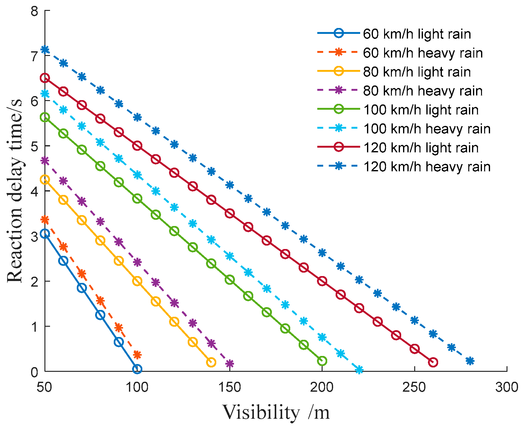
In the simulation environment configuration, we chose a heavy rain scenario with a traffic accident occurrence rate accounting for 60% [1]. Within this scenario, rainfall intensity ranges from 25 to 49.9 mm over a 24 h period. According to information from reference [7], the road surface friction coefficient for this scenario is established as φ = 0.3. Employing Formula (4), the delay response time is calculated to be t_f = 1.221 s. For the simulation setup, the ego vehicle is represented by a red rectangular block, designated with a velocity of v_ego = 10 m/s. The surrounding obstacle vehicles are depicted as blue rectangular blocks, with a set velocity of v_obs = 5 m/s.

We present two randomly generated simulation scenarios, as illustrated in Figure 13 and Figure 14. From these scenarios, it can be observed that considering visibility cost and neglecting visibility cost can lead to the generation of entirely distinct trajectories. Through thorough comparative analysis, we can discern that the incorporation of more accurate rainy day lane change boundary conditions, the establishment of feasible rainy day lane change regions, and the introduction of visibility cost functions during the dynamic programming phase collectively contribute to the observed differences.

In the lane change process spanning 0 m to 20 m, trajectories accounting for visibility cost exhibit a more conservative and secure nature when compared to trajectories disregarding visibility cost. On the other hand, during the lane change and collision avoidance phase spanning 20 m to 40 m, the integration of an enhanced safety distance constraint within the collision avoidance cost function often leads the ego vehicle to exhibit a tendency to distance itself from surrounding vehicles. This outcome aligns more closely with the experiential and behavioral habits of human drivers.

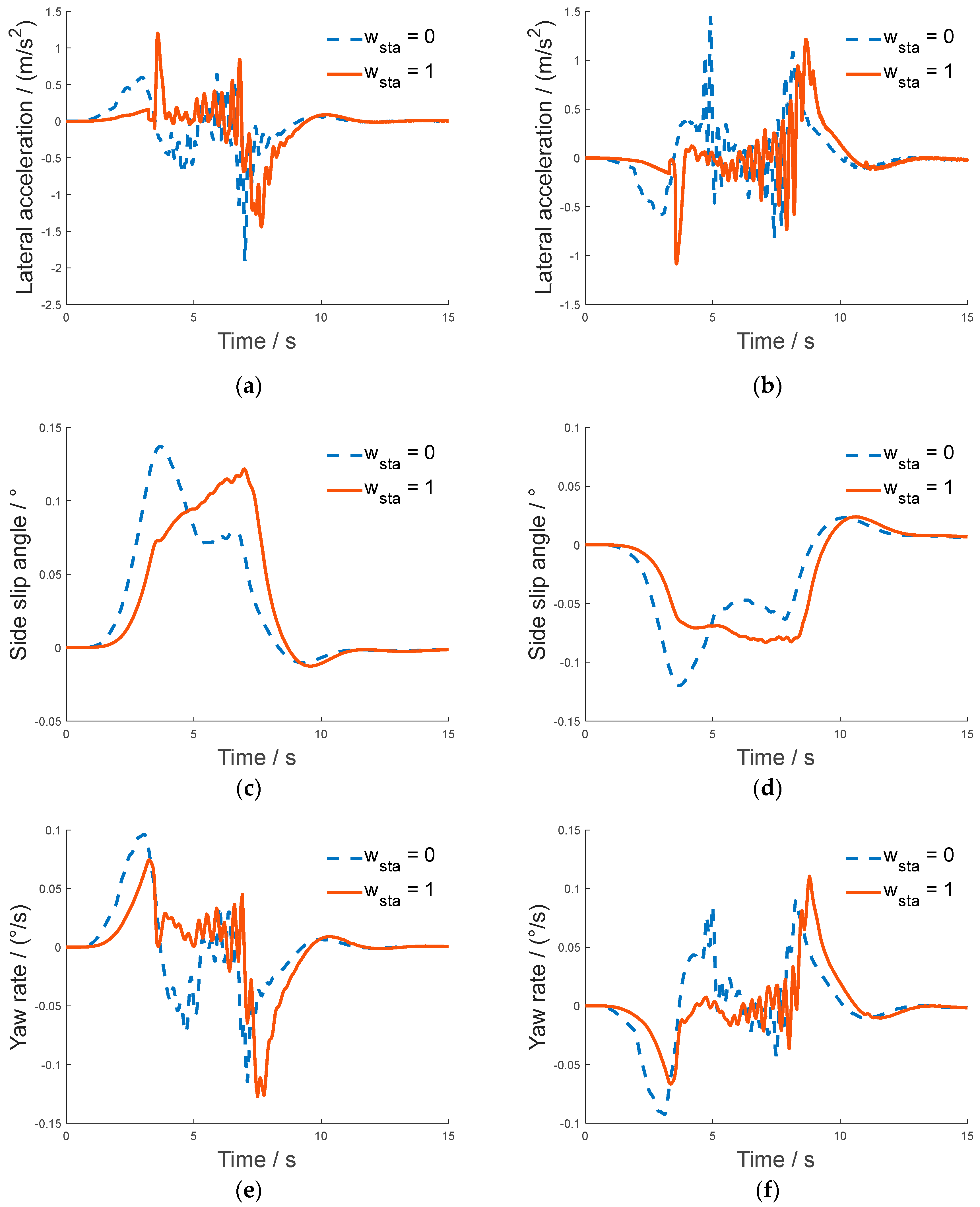
While focusing on the safety of lane changing under rainy conditions, comfort and maneuverability are of equal importance in vehicle lane change maneuvers. Therefore, in order to verify whether the algorithm generates trajectories with higher maneuverability and stability, this study shows the profiles of the vehicle states with or without considering the maneuverability objective function for both the left and right lane change scenarios under rainy conditions, as shown in Figure 15.

When assessing stability, lateral acceleration emerges as a pivotal evaluation metric, as manifested in Figure 15a,b. Throughout the lane change process, lateral acceleration consistently oscillates within the range of ±1.5 m/s². Thorough comparative analysis reveals that, with the introduction of a stability objective function during the quadratic programming phase, which is notably evident in the left/right lane change scenarios, the vehicle’s lateral acceleration curve exhibits a more pronounced reduction trend. Specifically, the peak lateral acceleration experiences a decrease of approximately 1 m/s² compared to the scenario where the stability objective function is not considered.

Furthermore, we investigated the sideslip angle in different scenarios, as depicted in Figure 15c,d. The variation in the sideslip angle reflects the extent of deviation between the vehicle’s travel direction and the road direction. In both lane change scenarios, the sideslip angle consistently oscillates within the range of ±0.15°. Notably, when considering the stability objective function, the sideslip angle curve exhibits smaller peaks in comparison to the scenario where stability considerations were absent, oscillating within the range of approximately ±0.1°. This indicates that the incorporation of the stability objective function during rainy day lane changing results in smoother fluctuations of the sideslip angle, contributing to an overall smoother lane change process.

In addition, the yaw rate serves as a vital parameter for assessing stability and comfort during the lane change process. As depicted in Figure 15e,f, the yaw rate curve remains within the range of ±0.1°/s throughout the entire process. In particular, at around 5 s, the yaw rate curve, influenced by the introduction of the stability objective function, exhibits a noticeable reduction in peak values. This implies that the incorporation of the stability objective function leads to a more stable yaw rate throughout the lane change process, thereby enhancing passenger comfort and overall stability.

6. Conclusions

In this paper, we introduce a trajectory planning algorithm for the lane changing of autonomous vehicles in rainy day scenarios for the safety and stability of the lane change operation of autonomous vehicles under adverse weather conditions.

(1) Introduction of friction coefficient and delayed reaction time. In this study, we first consider the slippery condition of the road on rainy days and introduce the friction coefficient and delayed reaction time as the key factors, to accurately calculate the safe distance for following and the safe distance for changing lanes and thereby to establish the boundaries of the feasible domain of lane changing on rainy days.

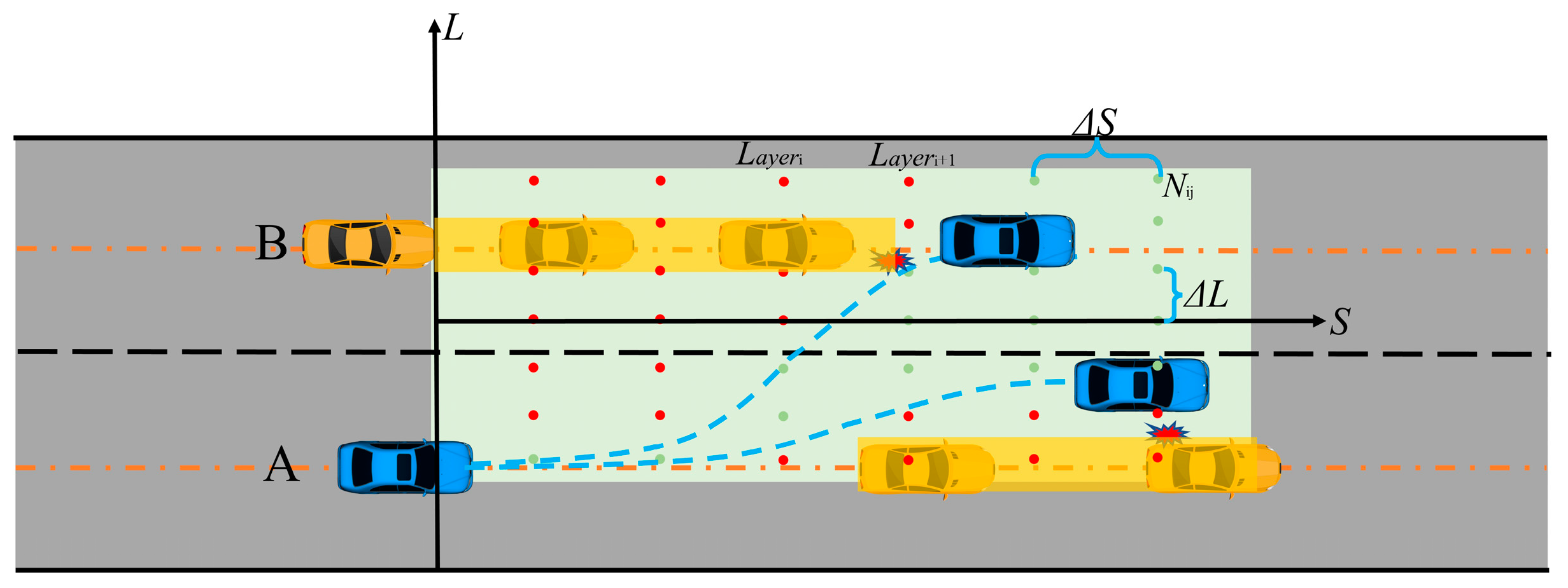
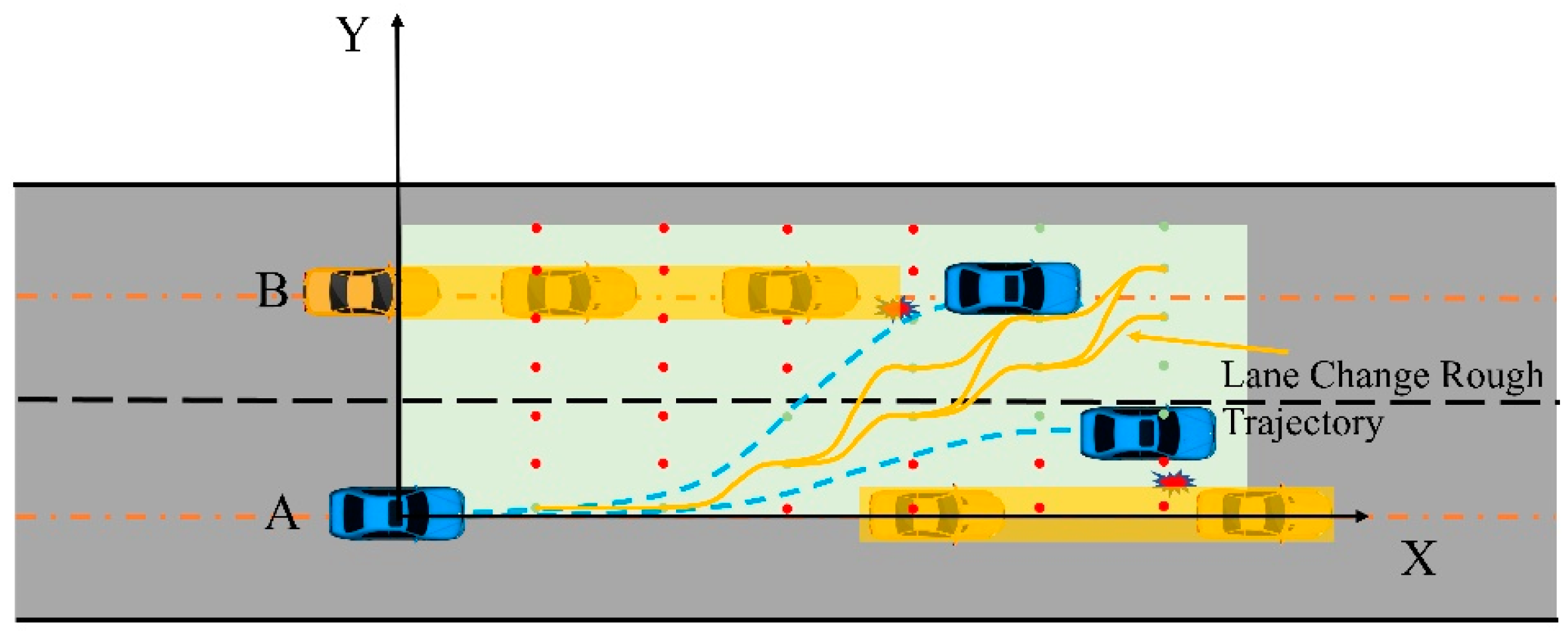
(2) Introduction of visibility cost function and improvement of safety distance constraints. A hierarchical trajectory planning strategy is adopted and dynamic programming is used to search for rough trajectories to obtain robust and safe initial solutions.

(3) The operation stability objective function is introduced. For the sideslip problem on a wet and slippery road, the quadratic programming algorithm is improved with the introduction of the stability objective function, which improves the smoothness of vehicle traveling and effectively reduces the potential risk of sideslip.

The simulation results show that the algorithm makes the host vehicle generate more conservative and safe trajectories in bad weather. It is more inclined to move away from the surrounding vehicles during the lane change obstacle avoidance phase. Meanwhile, the lateral acceleration varies within the range of ±1.5 m/s², the sideslip angle fluctuates within the range of ±0.15°, and the yaw rate is kept within the range of ±0.1°/s, fulfilling the requirements of comfort and stability. In this paper, although the environment and other influencing factors are considered, there is no real vehicle test under severe weather, and there are still complex weather environment situations that have not been considered. In the future, the lane change problem under different severe weather conditions can be investigated and more parameters and strategies can be explored to maintain the adaptability of the algorithm in diverse weather conditions. Additionally, in this paper, we only consider the host vehicle and the surrounding obstacle vehicles at a constant speed; in the next stage of research, we will consider the surrounding obstacle vehicles as having a variable speed in the speed planning stage of the host vehicle in order to adapt to more complex driving scenarios.

References

1. Yannis, G.; Theofilatos, A. A review of the effect of traffic and weather characteristics on road safety. Accid. Anal. Prev. 2014, 72, 244–256. [Google Scholar]
2. Pang, B.; Ren, N. CA model simulation of possible traffic accidents in rainy weather on highway curves. Chin. J. Saf. Sci. 2017, 7, 24–29. [Google Scholar]
3. Zhang, L.; Li, B.; Hao, Y.; Hu, H.; Hu, Y.; Huang, Y.; Chen, H. A Novel Simultaneous Planning and Control Scheme of Automated Lane Change on Slippery Roads. IEEE Trans. Intell. Transp. Syst. 2022, 23, 20696–20706. [Google Scholar] [CrossRef]
4. Kamgarpour, M.; Dadok, V.; Tomlin, C. Trajectory Generation for Aircraft Subject to Dynamic Weather Uncertainty. In Proceedings of the 2010 49th IEEE Conference on Decision and Control (CDC), Atlanta, GA, USA, 15–17 December 2010. [Google Scholar]
5. Peng, T.; Su, L.-L.; Guan, Z.W.; Hou, H.J.; Li, J.-K.; Liu, X.-L.; Tong, Y.-K.; Yu, B. Lane-Change Model and Tracking Control for Autonomous Vehicles on Curved Highway Sections in Rainy Weather. J. Adv. Transp. 2020, 2020, 8838878. [Google Scholar] [CrossRef]
6. Guo, L.; Ge, P.S.; Yue, M.; Zhao, Y.B. Lane Changing Trajectory Planning and Tracking Controller Design for Intelligent Vehicle Running on Curved Road. Math. Probl. Eng. 2014, 2014, 478573. [Google Scholar] [CrossRef]
7. Aung, M.Z.; Umeda, N. Investigation into control strategies for maneuvering in adverse weather conditions. Ocean. Eng. 2020, 218, 108170. [Google Scholar] [CrossRef]
8. Liu, Z.; Yu, C.; Wang, C.; Li, Q. Influence of fogy environment on expressway car-following safety. J. Chongqing Jiao Tong Univ. 2019, 38, 88–94. [Google Scholar]
9. Zhang, Z.; Zheng, L.; Li, Y.; Zeng, P.; Liang, Y. Structured road-oriented motion planning and tracking framework for active collision avoidance of autonomous vehicles. Chin. Sci. 2021, 64, 2427–2440. [Google Scholar] [CrossRef]
10. Tian, J.; Bei, S.; Li, B.; Hu, H.; Quan, Z.; Zhou, D.; Zhou, X.; Tang, H. Research on Active Obstacle Avoidance of Intelligent Vehicles Based on Improved Artificial Potential Field Method. World Electr. Veh. J. 2022, 13, 97. [Google Scholar] [CrossRef]
11. Yang, W.; Li, C.; Zhou, Y. A Path Planning Method for Autonomous Vehicles Based on Risk Assessment. World Electr. Veh. J. 2022, 13, 234. [Google Scholar] [CrossRef]
12. Liu, Y.; Sun, Y.; Cui, D.; Mophou, G. Optimum Path Tracking Control for the Inverse Problem of Vehicle Handling Dynamics Based on the hp-Adaptive Gaussian Pseudospectral Method. Math. Probl. Eng. 2021, 2021, 6631049. [Google Scholar] [CrossRef]
13. Yu, C.; Wang, Y.; Gao, F. Interval analysis method for safety distance of car-following. Trans. Chin. Soc. Agric. Mach. 2009, 40, 31–35. [Google Scholar]
14. Jiang, R.; Guo, Z.; Li, Z. Lane-changing safety model for deteriorative weather. J. Tongi Univ. 2011, 39, 529–533. [Google Scholar]
15. Konstantinos, M.; Markos, P. Motorway Path Planning for Automated Road Vehicles Based on Optimal Control Methods. Transp. Res. Rec. J. Transp. Res. Board 2018, 2672, 036119811878071. [Google Scholar]
16. Hegedus, F.; Becsi, T.; Aradi, S.; Gaspar, P. Motion Planning for Highly Automated Road Vehicles with a Hybrid Approach Using Nonlinear Optimization and Artificial Neural Networks. J. Mech. Eng. 2019, 65, 148–160. [Google Scholar] [CrossRef]
17. Svensson, L.; Bujarbaruah, M.; Kapania, N.; Törngren, M. Adaptive Trajectory Planning and Optimization at Limits of Handling. In Proceedings of the 2019 IEEE/RSJ International Conference on Intelligent Robots and Systems (IROS), Macau, China, 3–8 November 2019. [Google Scholar]
18. Chae, H.; Yi, K. Virtual target-based overtaking decision motion planning and control of autonomous vehicles. IEEE Access 2020, 99, 51363–51376. [Google Scholar] [CrossRef]
19. Pan, J.; Wang, J.; Xing, S. Dynamic Trajectory Planning and Optimization for Automated Driving on Ice and Snow Covered Road. IEEE Access 2023, 11, 36365–36378. [Google Scholar] [CrossRef]
20. Pang, M.B.; Ren, B.N. Effects of rainy weather on traffic accidents of a freeway using cellular automata model. Chin. Phys. B 2017, 26, 515–526. [Google Scholar] [CrossRef]
21. Chen, G.; Zhao, X.; Gao, Z.; Hua, M. Dynamic Drifting Control for General Path Tracking of Autonomous Vehicles. IEEE Trans. Intell. Veh. 2023, 8, 2527–2537. [Google Scholar] [CrossRef]
22. Chen, G.; Hua, M.; Zong, C.; Zhang, B.; Huang, Y. Comprehensive chassis control strategy of FWIC-EV based on sliding mode control. IET Intell. Transp. Syst. 2019, 13, 703–713. [Google Scholar] [CrossRef]
23. Yu, M.; Luo, Q.; Wang, H.; Lai, Y. Electric Logistics Vehicle Path Planning Based on the Fusion of the Improved A-Star Algorithm and Dynamic Window Approach. World Electr. Veh. J. 2023, 14, 213. [Google Scholar] [CrossRef]
24. Li, B.; Zhang, Y. Fast Trajectory Planning in Cartesian rather than Frenet Frame: A Precise Solution for Autonomous Driving in Complex Urban Scenarios. IFAC-Pap. OnLine 2020, 53, 17065–17070. [Google Scholar] [CrossRef]
25. Lim, W.; Lee, S.; Sunwoo, M.; Jo, K. Hierarchical Trajectory Planning of an Autonomous Car Based on the Integration of a Sampling and an Optimization Method. IEEE Trans. Intell. Transp. Syst. 2018, 19, 613–626. [Google Scholar] [CrossRef]
26. Barreiro, J.; Do, M.B.; Smith, D.E. In Intelligent UAS Sense-and-Avoid Utilizing Global Constraints. In Proceedings of the International Conference on Automated Planning and Scheduling, Portsmouth, NH, USA, 21–26 June 2014. [Google Scholar]
27. Elbanhawi, M.; Simic, M. Sampling-Based Robot Motion Planning: A Review. IEEE Access 2014, 2, 56–77. [Google Scholar] [CrossRef]
28. Li, L.; Liu, T.; Wang, F. Study on the impact of rainy day visibility on highway driving safety. Highway 2013, 5, 136–140. [Google Scholar]
29. Li, B.; Zhang, Y.; Feng, Y.; Zhang, Y.; Ge, Y.; Shao, Z. Balancing computation speed and quality: A decentralized motion planning method for cooperative lane changes of connected and automated vehicles. IEEE Trans. Intell. Veh. 2018, 3, 340–350. [Google Scholar] [CrossRef]
30. Federal Highway Administration. Flexibility in Highway Design; Federal Highway Administration: Washington, DC, USA, 1997.
Figure 1. Overall framework of this study.
Wevj 14 00252 g001
Figure 2. Profile of visibility versus rainfall intensity.
Wevj 14 00252 g002
Figure 3. Reaction delay time under different visibility conditions.
Wevj 14 00252 g003
Figure 4. Rainy weather lane change safety feasible region.
Wevj 14 00252 g004
Figure 5. Region schematic diagram of the follow−through process.
Wevj 14 00252 g005
Figure 6. Diagram of lane change process.
Wevj 14 00252 g006
Figure 7. Transformation to Frenet coordinate system, Where the red line indicates the reference line and the orange line indicates the lane center line.
Wevj 14 00252 g007
Figure 8. Sampling points within rainy weather lane change feasible region.
Wevj 14 00252 g008
Figure 9. The rough trajectory of lane change in Cartesian coordinates.
Wevj 14 00252 g009
Figure 10. Lane change trajectory clusters in Frenet coordinates, where the red lines are lane change rough trajectory candidates and the blue points are sampling points.
Wevj 14 00252 g010
Figure 11. Coarse lane change trajectory obtained via dynamic programming. In the illustration, the red lines depict the cluster of lane change trajectories, the green lines represent the coarse lane change trajectory, the blue points are sampling points, while the grey rectangles represent obstacle vehicles driving at a constant speed.
Wevj 14 00252 g011
Figure 12. Trajectory optimization process based on quadratic programming. (The process begins with a coarse trajectory as the initial solution and utilizes the lane centerline S as a reference line. The spatial coordinates are discretized into a coordinate system with a resolution of Δs. The upper and lower bounds of L are determined based on road boundaries and obstacle information. By solving for each Li, the precise trajectory is obtained. Where the orange line forms the discretised sampling space, the indigo curve is the rough trajectory, the magenta curve is the precise trajectory, and the green rectangle is the obstacle vehicle).
Wevj 14 00252 g012
Figure 13. Ego vehicle left lane change scenario.
Wevj 14 00252 g013
Figure 14. Ego vehicle right lane change scenario.
Wevj 14 00252 g014
Figure 15. State profiles of vehicle maneuverability ((a,c,e) are the vehicle state profiles for the left lane change scenario with or without considering the maneuverability objective function, and (b,d,f) are the vehicle state profiles for the right lane change scenario with or without considering the maneuverability objective function).
Wevj 14 00252 g015