Testing Scenario Identification for Automated Vehicles Based on Deep Unsupervised Learning

Abstract

Naturalistic driving data (NDD) are valuable for testing autonomous driving systems under various driving conditions. Automatically identifying scenes from high-dimensional and unlabeled NDD remains a challenging task. This paper presents a novel approach for automatically identifying test scenarios for autonomous driving through deep unsupervised learning. Firstly, US DAS2 NDD are leveraged, and the selection of data variables representing the vehicle state and surrounding environment is conducted to formulate the segmentation criterion. The isolation forest (IF) algorithm is then employed to segment the data, yielding two distinct types of datasets: typical scenarios and extreme scenarios. Secondly, a one-dimensional residual convolutional autoencoder (1D-RCAE) is developed to extract scenario features from the two datasets. Compared to four other autoencoders, the 1D-RCAE can effectively extract crucial information from high-dimensional data with optimal feature extraction capability. Next, considering the varying importance of different features, an information entropy (IE)-optimized K-means algorithm is employed to cluster the features extracted using 1D-RCAE. Finally, statistical analysis is performed on the parameters of each cluster of scenarios to explore their distribution characteristics within each class, and four typical scenarios are identified along with five extreme scenarios. The proposed unsupervised framework, combining IF, 1D-RCAE, and IE-improved K-means algorithms, can automatically identify typical and extreme scenarios from NDD. These identified scenarios can then be applied to test the performance of autonomous driving systems, enriching the library of automated driving test scenarios.

1. Introduction

The development of autonomous driving technology has increased the demand for diverse and realistic test scenarios. Naturalistic driving data (NDD) provide valuable information for testing autonomous driving systems under various driving conditions. Scene-based testing for autonomous driving is an effective approach used to reduce testing costs and improve testing efficiency. Well-known open-source datasets such as NGSIM [1], KITTI [2], and High-D [3] have been widely applied to scenario identification and validation for autonomous driving algorithms. By collecting and analyzing the NDD, a better understanding of the patterns in real driving environments can be achieved, providing valuable support for testing scenario construction. Additionally, the extracted test scenarios can be utilized to evaluate and compare the performance and limitations of autonomous driving systems, thereby guiding system optimization.

Numerous scholars have conducted related research on the identification of testing scenarios based on NDD. Some have placed significant emphasis on mining features from NDD, such as road types, road conditions, and traffic situations, in order to support the generation of test scenarios for automated driving. Gu et al. [4] employed NDD for scene graph generation, integrating external knowledge and image reconstruction techniques to enhance the accuracy and reliability of scene generation. Ries et al. [5] proposed a network structure that combines convolutional neural network (CNN) and long short-term memory network (LSTM) methods to identify scenes from videos. The positions of traffic participant and ego vehicle are encoded in a grid-based format. Z. Du et al. [6] extracted scenario features from NDD using LGBM decision trees and combined them with CIDAS accident data to restructure scenarios. Ding et al. [7] proposed the conditional multiple-trajectory synthesizer (CMTS), which combines normal and collision trajectories to generate safety-critical scenarios by interpolating them in the latent space. The method of extracting test scenarios from NDD has shown promising progress, but it still faces numerous challenges. These challenges primarily include accurately identifying scenes from massive datasets, automating the annotation process for efficient data labeling, and handling diverse data sources and formats. Consequently, the development of ways to effectively utilize NDD to improve the accuracy and efficiency of scenario identification has become a critical concern for researchers. Therefore, there is a pressing need in both industry and academia for an automated data labeling approach in order to reduce labeling costs.

The existing unsupervised and semi-supervised methods [8,9] can reduce labeling efforts but are not suitable for handling large amounts of high-dimensional time-series data. Additionally, existing research mostly focuses on specific scenarios based on NDD, such as lane changing [10,11] and car following [12,13]. This approach cannot fully utilize the scenario information contained in NDD. Thus, the challenge is to identify different types of scenes on a large scale from massive NDD. This problem can be addressed using rule-based [14] and machine learning-based approaches [15,16,17,18]. Rule-based approaches rely on expert experience. Zhao et al. [19] modeled driving scenarios based on ontology and integrated data from multiple sensors. They constructed a rule library for driving scenarios by incorporating expert knowledge and legal regulations. This was leveraged to assist in the development and testing of various functions in intelligent connected vehicles. Sun et al. [20] identified dangerous scenarios from NDD by setting thresholds for parameters such as speed and acceleration. Wachenfeld et al. [21] introduced a dangerous scenario extraction method based on the worst-case collision time. The fundamental principle of identifying test scenarios through machine learning lies in mining the intrinsic features and patterns within the data for scene classification. Tan et al. [22] inputted the current state of the autonomous vehicle and the high-definition map into an LSTM network and trained the model using NDD to generate natural driving scenarios. Rocklage et al. [23] presented a retrospective-based approach for automatic scene extraction and generation that was capable of randomly generating static or dynamic scenes. Fellner et al. [24] proposed a heuristic-guided branch search algorithm for scene generation. Spooner et al. [25] introduced a novel method called ped-cross generative adversarial network (Ped-Cross GAN) to generate pedestrian crosswalk scenes. Additionally, importance sampling [26] and Monte Carlo search [27] methods have also been widely applied in efforts to generate critical scenarios.

Despite the efficiency and simplicity of the rule-based approach, subjective rules and threshold settings are often introduced during rule formulation. However, these are not generalizable approaches for different NDD, and their use can result in subjective errors. In contrast, machine learning-based methods can automatically learn and discover features and identify scenarios from data with better adaptiveness. Therefore, applying machine learning theory in scene identification is becoming one of the mainstream methodologies in the present and will be important into the future.

To obtain different scenarios under extreme and typical driving conditions, it is necessary to divide original NDD into extreme and typical data subsets. Isolation forest (IF) [28] is a fast, efficient, and unsupervised data segmentation method. Its fundamental principle involves randomly partitioning the dataset and applying the depth of trees to determine the typical and extreme data. Due to the high dimensionality of the raw data, the use of direct training would result in inefficiency. Therefore, autoencoders [29] have been widely employed in the field of feature extraction. The conventional autoencoder (AE) employs fully connected layers, which results in a large number of parameters. When dealing with high-dimensional data, this method is prone to overfitting and lacks local perception. In contrast, convolutional neural networks consist of convolutional layers and pooling layers. By introducing convolutional kernels, parameter sharing can be achieved, reducing the number of model parameters and accelerating the training process. Additionally, increasing the number of network layers can cause training difficulties and higher training costs, as well as issues like gradient vanishing or exploding. The application of residual learning [30] can help to propagate gradients more effectively within the network, thereby improving its training performance.

Identifying test scenarios is crucial in the research for and development of autonomous driving systems. The identified test scenarios can be adopted to objectively evaluate the performance of autonomous driving algorithm. By testing the behavior and performance of autonomous vehicles in various scenarios, a better understanding of the algorithm’s strengths and limitations can be gained, guiding its improvement and optimization. Different test scenarios may involve varying risks and challenges. Accurately identifying and categorizing these scenarios can assist autonomous vehicles to proactively responding to potential hazards, thereby ensuring safety. Identifying test scenarios based on the available data resources is a critical issue that requires urgent attention in the development of autonomous driving technology.

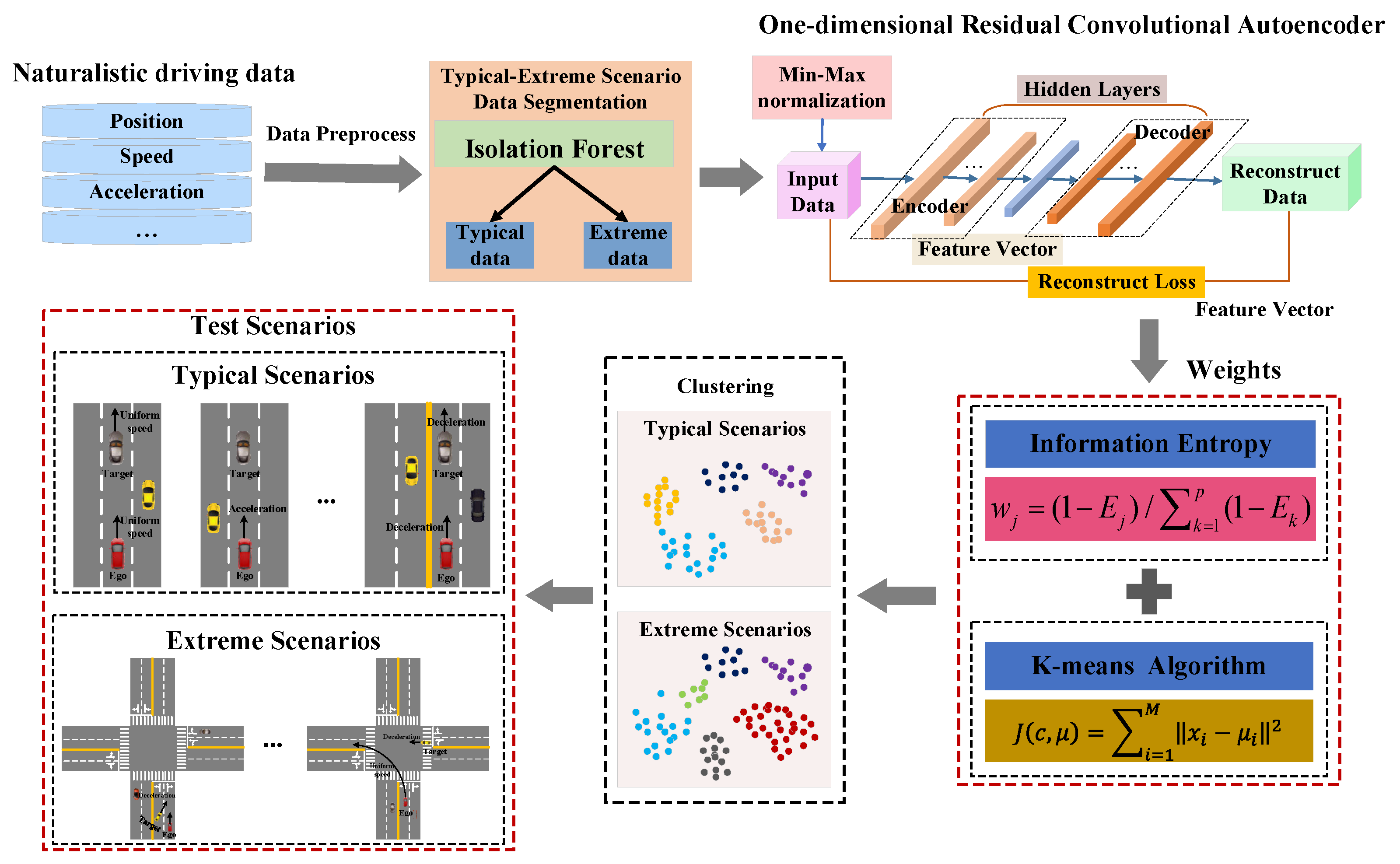
This paper addresses the challenges of large-scale and complex unlabeled NDD by proposing a deep unsupervised learning framework that combines IF, one-dimensional residual convolutional autoencoders (1D-RCAE), and information entropy (IE)-optimized K-means algorithms for autonomous driving testing scenario identification. Additionally, this method exhibits robustness to the complex noise and high-dimensional features present in NDD. The main contributions of this study are as follows: (1) Utilizing IF to achieve the segmentation of typical and extreme driving scenarios, resulting in separate datasets for the extraction of typical and extreme scenes. (2) Designing a novel neural network, the 1D-RCAE, which can learn and extract features from data without the need for labels, in contrast to traditional machine learning methods. (3) The residual learning mechanism is introduced to optimize the training process and enhances the feature extraction capability of the network. (4) The application of IE optimizes the K-means algorithm, enhancing the accuracy and robustness of the clustering process. The framework of the proposed method is shown in Figure 1.

2. Methodology

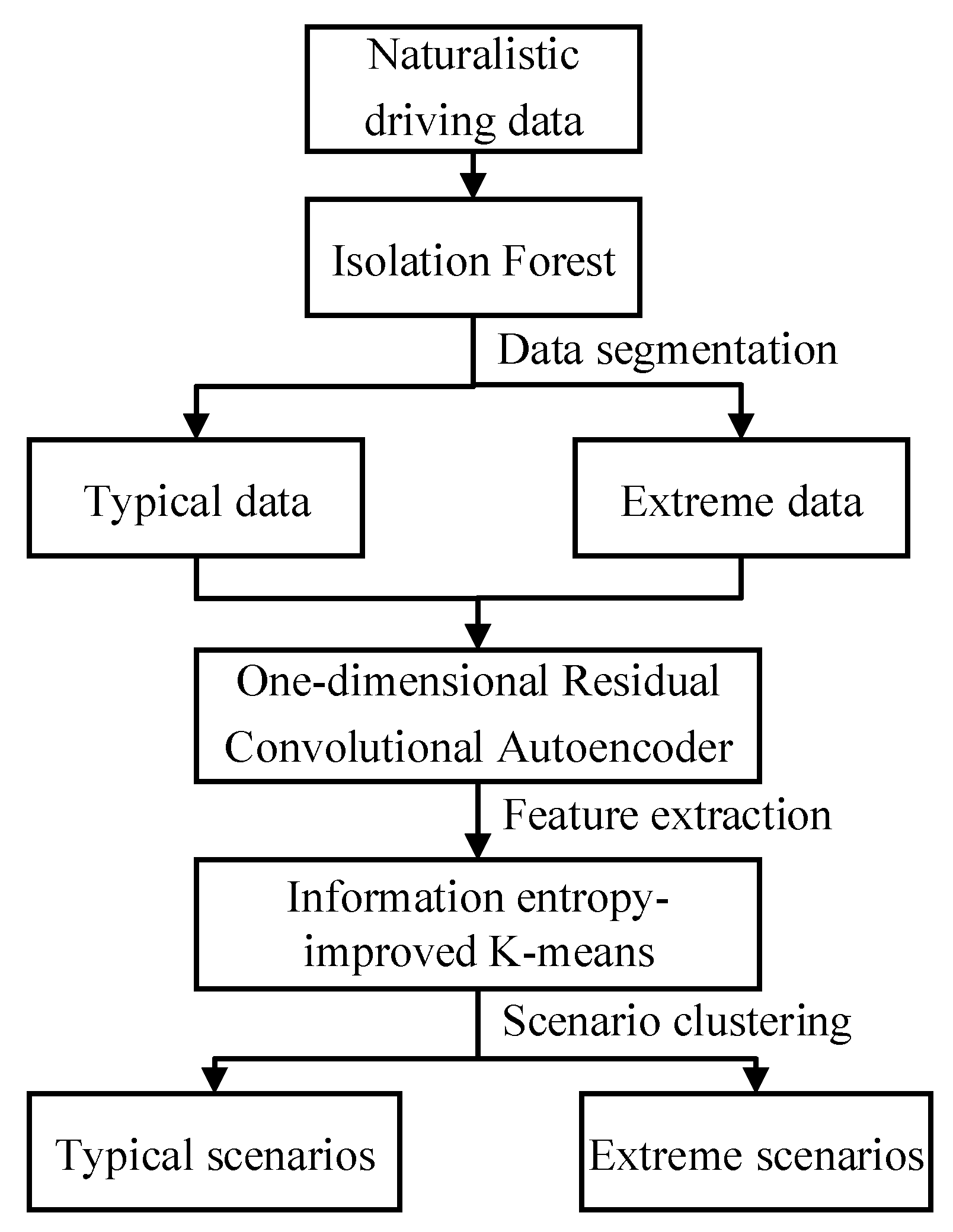
In this section, a novel scene recognition method is proposed for accurately classifying different traffic scenes, and the flow chart of the proposed methodology is shown in Figure 2.

2.1. Typical–Extreme Scenario Data Segmentation Based on Isolation Forest

The IF algorithm is applied to divide the original dataset into two parts: extreme data and typical data. The specific process of the IF algorithm is as follows.

(1)

Building isolation forest: an isolation forest is composed of multiple randomly partitioned binary trees.

(2)

Calculate the path length h of a binary tree $h(x)$: the path length $h(x)$ can be calculated as,

$$h(x)=e+C(T.size)$$

(1)

where $e$ denotes the number of edges traversed from the root node to a leaf node during the process of obtaining the sample $x$ in a tree. $C(T.size)$ represents the average path length of a binary tree constructed, with $T.size$ indicating the number of sample data.

(3)

Deviation measurement of extreme points: calculate the expected value $E(h(x))$ and variance $S(h(x))$ of the outlying degree of all samples, and then obtain the extreme data that deviate from the expected value and variance.

After computing the binary tree forest, normalize $E(h(x))$ by $C(n)$, with the $C(n)$ expressed as,

$$C(n)=2H(n-1)-(2(n-1)/n)$$

(2)

where $n$ is the number of data samples and $H(\ast )$ is the harmonic number, which can be represented as,

$$H(\ast )=\ln (n-1)+\xi$$

(3)

where $\xi$ is the Euler’s constant, with a value of 0.5772156649. It is important to note that the given Euler’s constant is an approximate value.

The degree of extreme in data can be represented as,

$$S(x,n)=2^{-\frac{E(h(x))}{C(n)}}$$

(4)

2.2. Scene Feature Extraction Based on One-Dimensional Residual Convolutional Autoencoder

The typical scenario data and extreme scenario data, obtained after the segmentation-based application of the IF algorithm, have high dimensions. Therefore, a convolutional autoencoder (CAE) is designed based on AE for feature extraction. Meanwhile, by incorporating residual learning into the CAE, a 1D-RCAE network is constructed. This can mitigate problems that arise with increasing network depth, such as vanishing or exploding gradients. The residual block can be defined as follows.

$$y=F(x,\{W_i\})+x$$

(5)

where $x$ and $y$, respectively, represent the input and output of the module. $F(•)$ represents the residual mapping to be learned, and $W_i$ denotes the parameters of the module.

As shown in Figure 3, residual learning employs a residual mapping function $F(X)=H(X)-X$ instead of learning the potential mapping $H(X)$ of the input at that layer. By introducing skip connections, which connect the input $X$ to the output of the module through identity mapping, gradients can be better propagated, thereby addressing the training issues of deep convolutional networks and improving network performance. This enables better capture of high-level features in the input data. Several existing network models, such as Inception-V4 [31] and Res-Next [32], have incorporated residual learning to enhance their performance.

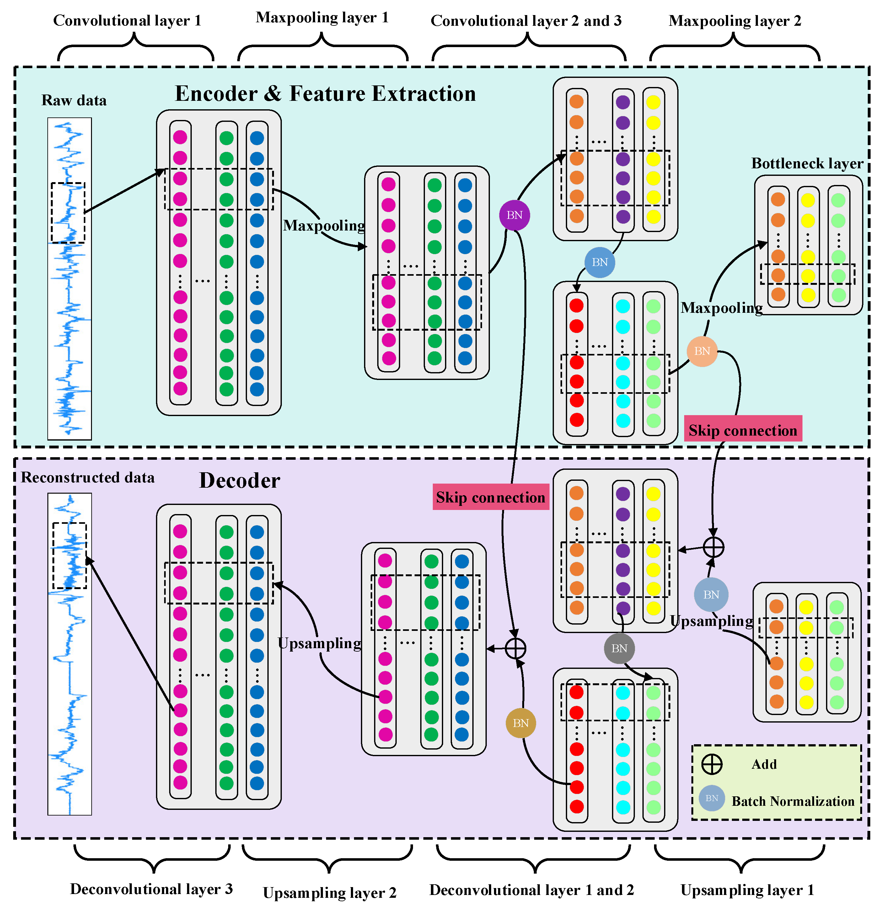
The feature extraction model based on the 1D-RCAE is shown in Figure 4. The encoder consists of convolutional layers and max pooling layers, while the decoder consists of deconvolutional layers and upsampling layers. The bottleneck layer denotes feature representation.

In order to reduce the number of learning parameters of the network and effectively reduce the dimensionality of the input data, convolutional kernels of size 1 × 4 and 1 × 6 with a stride of 1 are deployed in the one-dimensional convolutional layer. The sizes of the two max pooling layers are 2 and 4, respectively. Moreover, a convolutional kernel of size 1 × 1 with a stride of 1 makes up the bottleneck layer. The specific parameter values of the 1D-RCAE network are shown in

Table 1. The network parameters of 1D-RCAE.

	Parameters	Value
Encoder	convolutional layer 1	kernel_size: 1 × 4, strides: 1
	max pooling layer 1	size = 2
	convolutional layer 2	kernel_size: 1 × 1, strides: 1
	convolutional layer 3	kernel_size: 1 × 6, strides: 1
	max pooling layer 2	size = 4
	bottleneck layer 1	kernel_size: 1 × 1, strides: 1
Decoder	bottleneck layer 2	kernel_size: 1 × 1, strides: 1
	upsampling layer 1	size = 4
	deconvolution layer 1	kernel_size: 1 × 1, strides: 1
	deconvolution layer 2	kernel_size: 1 × 6, strides: 1
	upsampling layer 2	size = 2
	deconvolution layer 3	kernel_size: 1 × 4, strides: 1

.

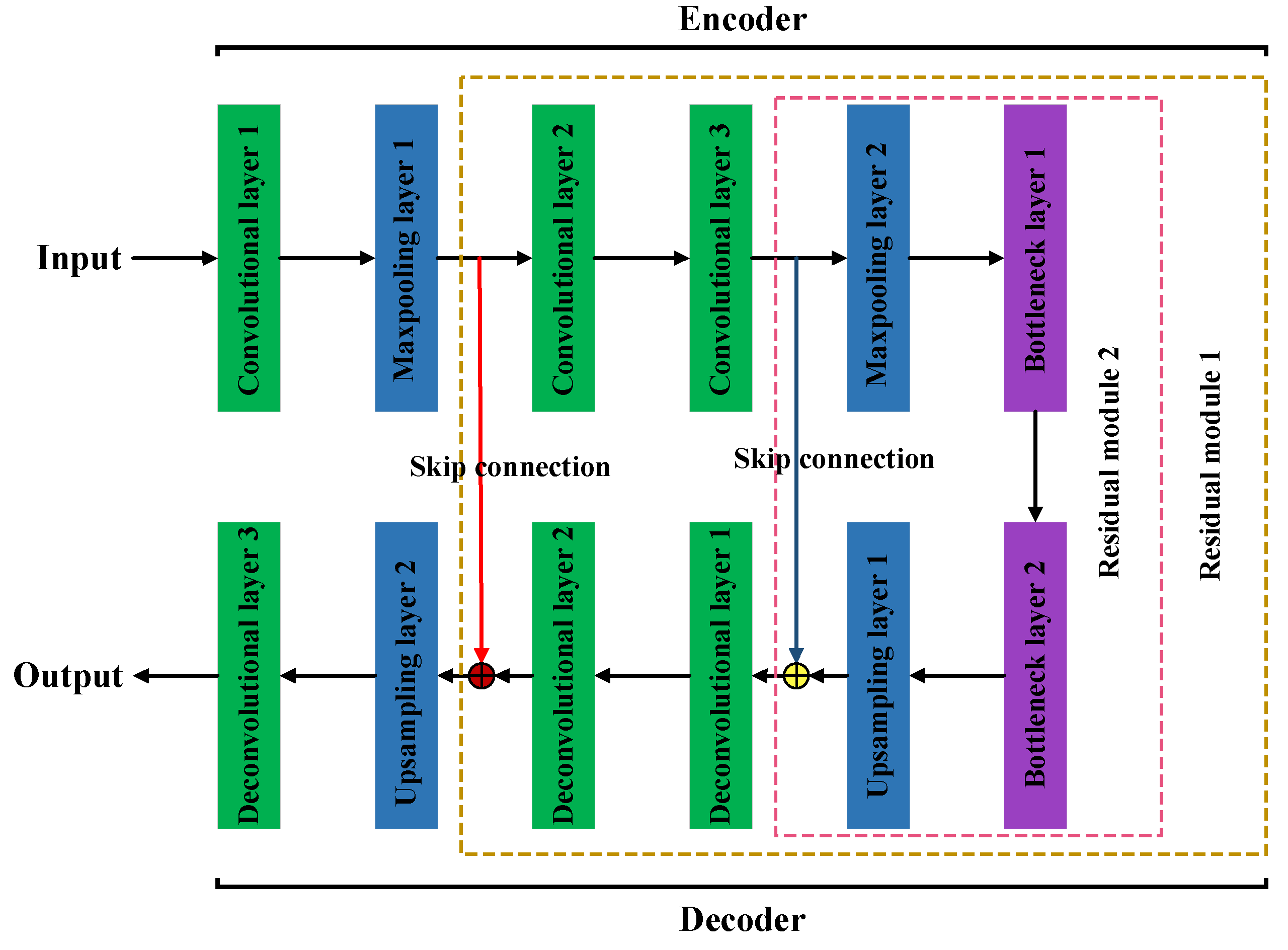
As shown in Figure 5, the 1D-RCAE consists of two residual modules. In the first residual module, the output of the first max pooling layer in the encoder is added to the output of the deconvolutional layer 2 in the decoder via a skip connection. This results in the development of new features that serve as the input to upsampling layer 2. The input of upsampling layer 2 can be expressed as

$$x_{u2}=P_1(C_1(x_{in}))+D_2(y_{D_1})$$

(6)

where $x_{u2}$ represents the input of upsampling layer 2, $P_1$ stands for max pooling layer 1, $C_1$ stands for convolutional layer 1, $D_2$ denotes deconvolutional layer 2, $x_{in}$ represents the original input data and $y_{D1}$ denotes the output of deconvolutional layer 1.

In the second residual module, the output of convolution layer 3 is added to the output of upsampling layer 1 through a skip connection to obtain a new feature, which serves as the input to deconvolution layer 1. The input of deconvolution layer 1 can be expressed as,

$$x_{D1}=C_3(y_{C2})+U_1(y_{B2})$$

(7)

where $x_{D1}$ represents the input of deconvolution layer 1, $C_3$ stands for convolutional layer 3, $U_1$ stands for upsampling layer 1, $y_{C2}$ represents the output of convolutional layer 2 and $y_{B2}$ denotes the output of bottleneck layer 2.

During training, the one-dimensional convolution process can be represented as,

$$x_i^l=\delta ({\displaystyle \sum _{i=1}^N{x}_i^{l-1}\times w_i^l+b_i^l})$$

(8)

where $\delta (•)$ represents the activation function, $x_i^l$ and $x_i^{l-1}$, respectively, represent the i-th feature vector of the l-th and (l − 1)-th convolutional layers, and $w_i^l$ denotes the weights between the convolutional kernel and the input data. $b_i^l$ stands for the bias term and $N$ represents the dimension of the input data in the convolutional layer.

To prevent lower training efficiency due to the gradual dispersion of data distribution resulting from shifts in internal variables after multiple convolutions, a batch normalization (BN) layer [33] is introduced after each convolutional layer. If the batch input data value $x$ is set to $B=\{x_1,x_2,\dots ,x_m\}$, the calculation process of the BN layer is as follows.

$${\mu }_{\beta }=\frac{1}{m}{\displaystyle \sum _{i=1}^m{x}_i}$$

(9)

$${\sigma }_{\beta }^2=\frac{1}{m}{{\displaystyle \sum _{i=1}^m(x_i-{\mu }_{\beta })}}^2$$

(10)

$${\widehat{x}}_i=\frac{x_i-{\mu }_{\beta }}{\sqrt{{\sigma }_{\beta }^2+\epsilon }}$$

(11)

$$y_i=\gamma {\widehat{x}}_i+\beta \equiv B{N}_{\gamma ,\beta }(x_i)$$

(12)

where ${\mu }_{\beta }$ represents the mean of batch processed data, ${\sigma }_{\beta }^2$ represents the variance of batch processed data, ${\widehat{x}}_i$ denotes the normalized data, and $y_i$ stands for the normalized network response. $\gamma$ and $\beta$ are the scale factor and shift factor, respectively, which are learned during the training of the network.

The activation function of the 1D-RCAE adopts the $ReLU$ activation function, and it can be expressed as,

$$ReLU(x)=\max (0,x)$$

(13)

The 1D-RCAE learns features by reconstructing the input data, and its loss function is defined as follows.

$$Loss=\frac{1}{N}{{\displaystyle \sum _{i=1}^N‖y_i-x_i‖}}^2$$

(14)

where $x_i$ stands for the inputs of the encoder and $y_i$ represents the outputs of the decoder.

2.3. K-Means Algorithm Based on Information Entropy Optimization

K-means is a commonly imposed unsupervised machine learning classification algorithm. In the clustering process, it utilizes the Euclidean distance as a measure of similarity between data points. A smaller value of the Euclidean distance indicates a higher degree of similarity. The calculation of Euclidean distance can be represented as,

$$d(x,C_i)=\sqrt{{\displaystyle \sum _{j=1}^n{(x_j-C_{ij})}^2}}$$

(15)

where $x$ represents the input data, $C_i$ denotes the i-th cluster center, $n$ represents the data dimension, $x_j$ and $C_{ij}$, respectively, stand for the j-th attribute value of the input data $x$ and the cluster center $C_i$.

The traditional K-means algorithm does not consider the weights of different features, assuming that all features are equally important. This can lead to poor clustering performances in certain situations. Therefore, IE is introduced to assign different weights to different features [34], thereby improving the accuracy and robustness of clustering. The calculation process of IE is as follows.

(1)

Standardize $x_{ij}$ with attribute $j$ for sample $i$, usually applying the min–max method for data standardization. The min–max method can be described as,

$$x_{ij}^{\prime }=\frac{x_{ij}-{\min }_i(x_{ij})}{{\max }_i(x_{ij})-{\min }_i(x_{ij})}$$

(16)

(2)

Calculate the proportion of the i-th sample in feature $j$.

$$p_{ij}=x_{ij}^{\prime }/{\displaystyle {\sum }_{i=1}^n{x}_{ij}^{\prime }}$$

(17)

(3)

Calculate the IE of $n$ samples in the feature $j$.

$$E_j=-\frac{1}{\ln n}{\displaystyle {\sum }_{i=1}^n{p}_{ij}\ln p_{ij}}$$

(18)

(4)

Calculate the weight of the j-th feature.

$$w_j=(1-E_j)/{\displaystyle {\sum }_{k=1}^p(1-E_k)}$$

(19)

where $p$ denotes the number of features.

By introducing IE to calculate weights, the dispersion and uncertainty of data within clustering clusters can be better measured. A smaller IE corresponds to a higher weight, indicating that the feature is more important for distinguishing different samples. A larger IE corresponds to a lower weight, indicating that the feature is less important for distinguishing different samples.

3. Data Collection and Experiments

3.1. Datasets and Data Processing

NDD from DAS2, collected using the safety pilot model deployment (SPMD) [35] data collection system of the US Department of Transportation, are used in our research. Compared to datasets such as NGSIM and High-D, the DAS2 dataset offers a wide range of road conditions, including urban, rural, and highway settings, providing a comprehensive representation of real-world driving scenarios. These data are collected with a sampling frequency of 10 Hz and cover a geographic range of longitude (−83.91°, −83.54°) and latitude (42.17°, 42.43°).

Considering that different variables in the data have different dimensions and value ranges, their direct implementation would affect the training effectiveness of the model. Therefore, to improve the training effectiveness and stability of the model, it is necessary to normalize the data. This paper applies the min–max normalization method, which linearly transforms the data for the purpose of mapping it into the range [0, 1]. The formula for min–max normalization is expressed as follows,

$$x^{\prime }=\frac{x-x_{\min }}{x_{\max }-x_{\min }}$$

(20)

where $x^{\prime }$ is the normalized data, $x$ is the original data, and $x_{\min }$ and $x_{\max }$ are the minimum and maximum values of that variable in the data, respectively.

3.2. Typical—Extreme Scenario Data Segmentation

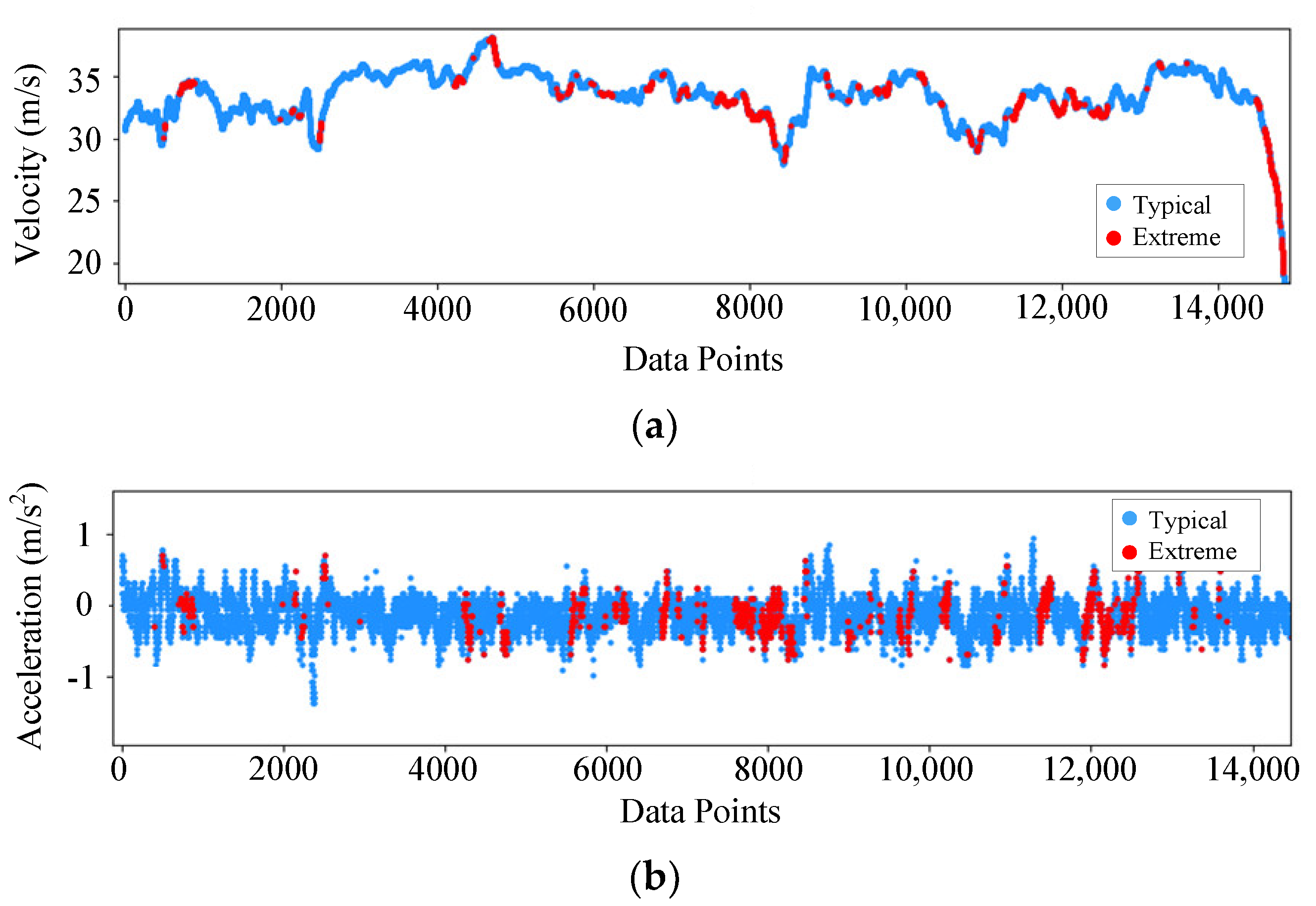
When leveraging IF to partition data, eight variables related to vehicle kinematics and the surrounding driving environment are selected as input data for partitioning. The eight variables are as follows: velocity, acceleration, steering wheel angle, yaw rate, relative lateral position, relative longitudinal position, relative lateral velocity, and relative longitudinal velocity. IF assigns a label of −1 or 1 to each data point based on the calculated results. A label of −1 indicates extreme scenario data, while 1 indicates typical scenario data. Taking the segmentation results of velocity and acceleration as examples, the segmentation results are visualized in Figure 6. It can be observed that the red points are located near the peaks of each acceleration and velocity change interval. This suggests that when the vehicle experiences large changes in acceleration and velocity, IF classifies it as extreme data.

Typical scenario data account for approximately 90% of the total data in the segmented dataset, while extreme scenario data comprise approximately 10% of the total. The segmentation results effectively reflect the driving behavior of vehicles to a certain extent, and the results align with the proportion of normal driving behavior and abnormal driving behavior in NDD. In this study, a scenario is defined as an overall description of the interaction between a vehicle and its surrounding environment during a certain period of time. When the continuous driving data of a vehicle exceed 0.5 s [36], they constitute a driving event, and the driving event, together with the surrounding environment, constitutes a scenario. Therefore, after completing data segmentation, driving events are extracted separately from the typical dataset and the extreme dataset. This resulting in 5584 driving events being obtained from the typical dataset, with a further 1274 driving events extracted from the extreme dataset.

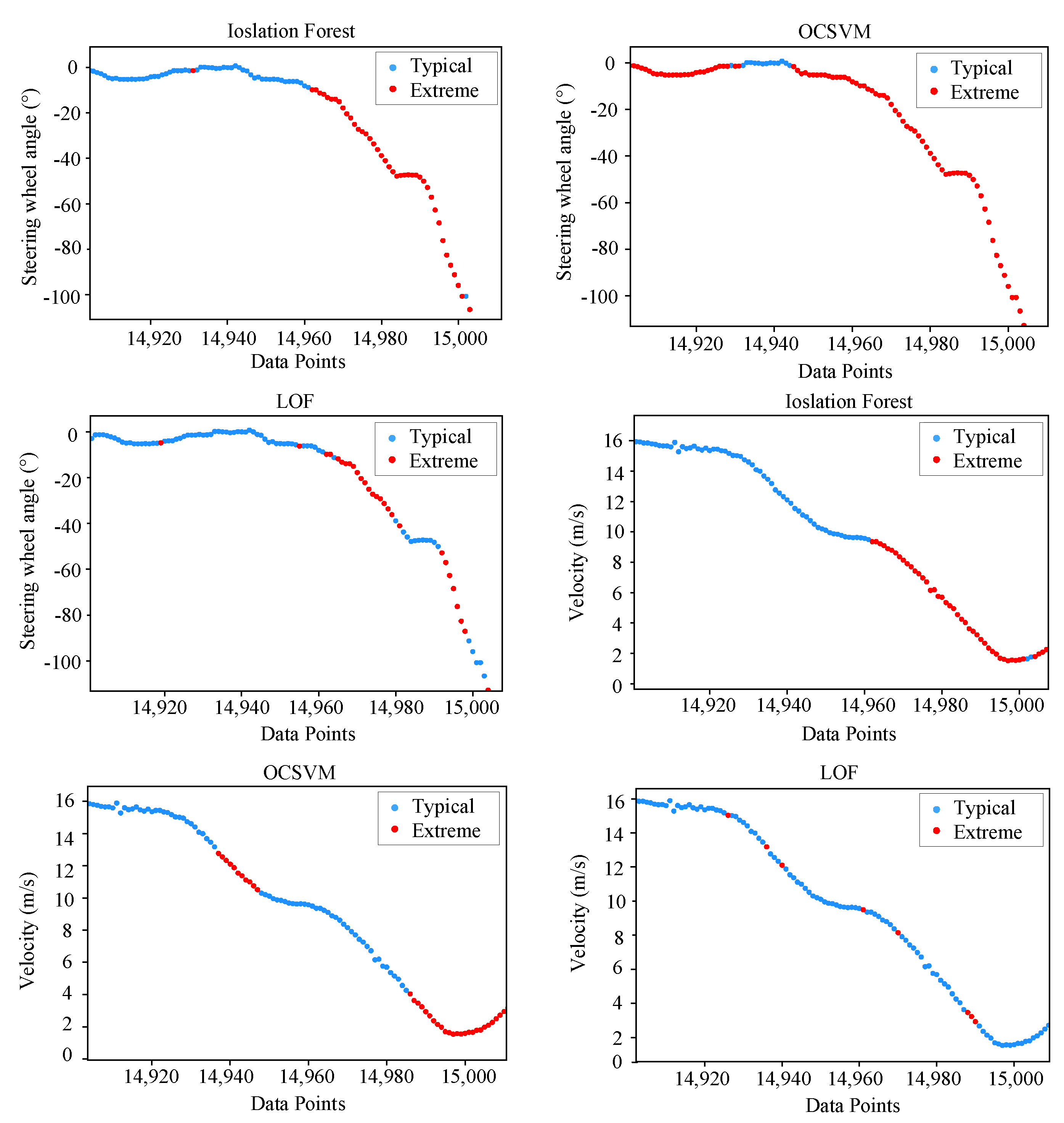
Despite obtaining good results by conducting IF for data segmentation, in order to further demonstrate the superior performance of the IF, a comparison is made between IF, local outlier factor (LOF) [37], and one-class support vector machine (OCSVM) [38] methods in terms of steering wheel angle and velocity, as shown in Figure 7. From the segmentation results, it can be observed that IF designates the data with large variations in steering wheel angle and velocity as extreme data, while the segmentation results of LOF and OCSVM lack interpretability.

3.3. Scenario Feature Extraction

To verify the proposed 1D-RCAE network feature extraction model, an experimental environment is constructed to combine Tensorflow 2.2.0 and Keras 2.3.1 (Google LLC, Mountain View, CA, USA) on a Windows 11 operating system (Microsoft Corporation, Redmond, WA, USA). The network model is built using Python 3.7 (Anaconda Inc, Austin, TX, USA). The hardware environment for the experiments consists of a processor of 12th Gen Intel(R) Core(TM) i7-12700H with 2.30 GHz (Intel Corporation, Santa Clara, CA, USA) and a GPU of NVIDIA GeForce RTX3050 (NVIDIA Corporation, Santa Clara, CA, USA).

The Adam optimizer based on backpropagation is adopted for optimization in the training process. The mean-squared error (MSE) method is applied as the loss function to evaluate the model. In addition, a weight decay term is added to the loss function to control the degree of weight decay and prevent the network from overfitting. The network training parameters are ultimately determined through multiple experiments using different parameter settings. The initial learning rate, regularization factor, momentum parameter and training epochs are set to 0.001, 0.1, 0.9 and 400, respectively. The specific network training parameters are shown in

Table 2. Training parameters of 1D-RCAE.

Parameters	Values
Network structure of encode layer	conv-pooling-conv-conv-pooling-conv
Initial learning rate	0.001
Optimizer	Adam
Activation function	ReLu
Loss function	MSE
$\lambda$	0.05
Momentum	0.9
Epochs	400
Batch size	32

.

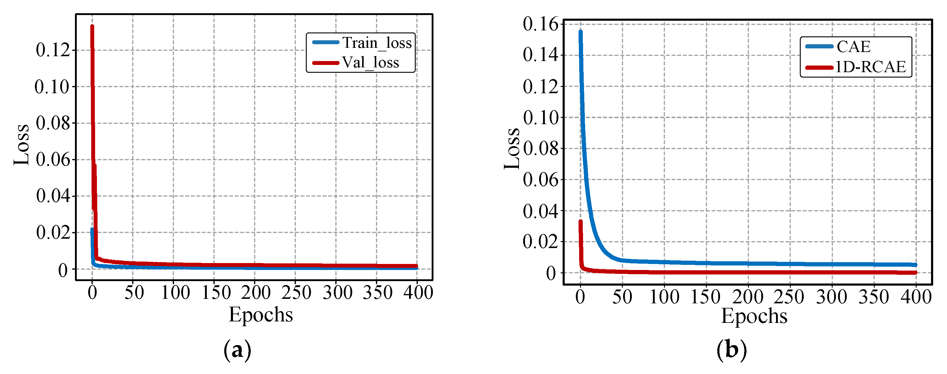
The input of 1D-RCAE comprises original data, encompassing velocity, acceleration, steering wheel angle, vehicle position, turn signal, relative distance, relative velocity, target motion state, and other relevant features. The output is the reconstructed data of the original input, which maintain the same dimensions as the input data. In this paper, the required features are the output data of the encoder, specifically the data from the bottleneck layer 1, as illustrated in Figure 5. Figure 8a shows the loss variation during the training and validation processes of 1D-RCAE. Analysis reveals that the training loss for the 1D-RCAE is 0.0009, while the validation loss converges to 0.0011. This indicates that the model is capable of effectively extracting data features and reconstructing the original data. Finally, the original data are represented as three-dimensional features by 1D-RCAE, as shown in

Table 3. The three-dimensional features extracted by 1D-RCAE.

	Feature 1	Feature 2	Feature 3
0	0.19868	1.28456	2.54810
1	0.19664	1.29419	2.53582
2	0.19499	1.02378	2.44288
3	0.19685	0.98529	2.46010
4	0.19582	1.03302	2.47379
…	…	…	…

. These features to some extent can represent the original high-dimensional data.

To illustrate the performance of the 1D-RCAE compared to the original CAE, the changes in their loss values during training are compared, as shown in Figure 8b. From the comparison, it can be observed that the use of 1D-RCAE delivered enhanced performances compared to the original version. The network converges faster and achieves lower convergence loss.

3.4. Scenario Clustering

The features extracted using 1D-RCAE are applied to cluster and the different feature weights of typical scenarios and extreme scenarios obtained through the calculation of IE are shown in

Table 4. Feature weights of typical scenarios and extreme scenarios.

Scenarios	Features	Weights
Typical scenarios	Feature 1	0.1371
	Feature 2	0.1665
	Feature 3	0.6964
Extreme scenarios	Feature 1	0.2155
	Feature 2	0.2251
	Feature 3	0.5594

.

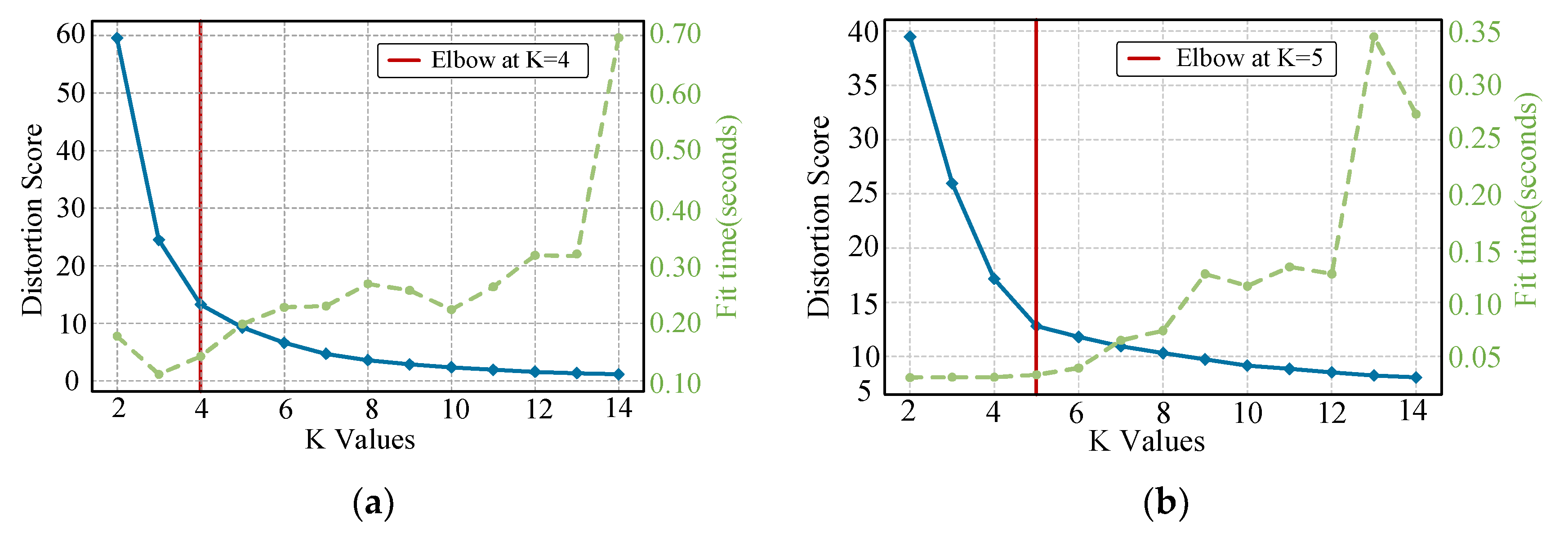
The number of clusters K has a significant impact on clustering performance. Setting K value to be too small or too large will result in poor clustering results. In this study, the “Elbow method” is applied to determine the value of K. The IE-optimized K-means algorithm is applied to the features, and elbow plots are generated for different K values. As illustrated in Figure 9, the optimal number of clusters for typical scenarios is 4, whereas it is 5 for extreme scenarios.

4. Results and Analysis

4.1. Performance Comparison of Different Feature Extraction Networks

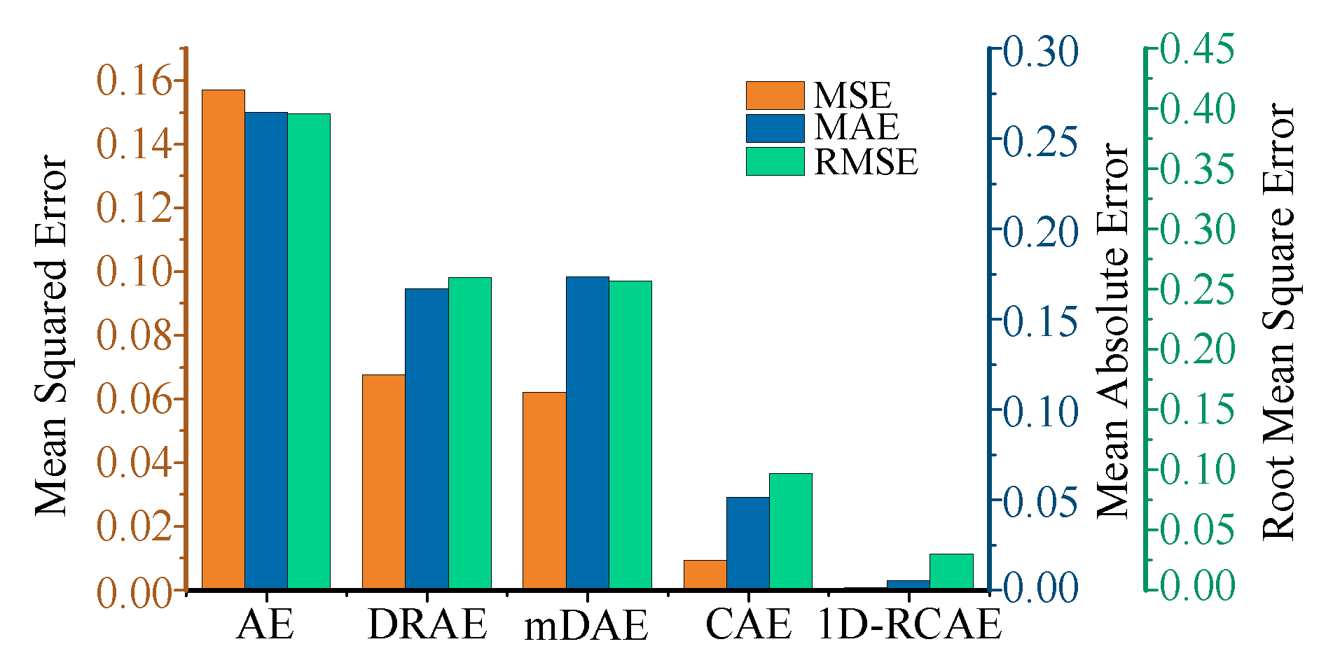
To compare the performance of 1D-RCAE with other types of autoencoders under the same data and experimental conditions, the performances of AE, deep regularized autoencoder (DRAE), marginalized denoising autoencoder (mDAE), CAE, and 1D-RCAE are compared. Figure 10 illustrates the comparative results of these five networks in terms of MSE, mean absolute error (MAE), and root-mean-squared error (RMSE), which are three evaluation metrics.

From the Figure 10, it can be concluded that the 1D-RCAE has lower MSE, MAE, and RMSE values compared to other networks. This indicates that the 1D-RCAE designed in this paper possesses superior feature extraction capability. It is capable of uncovering deep-level features from high-dimensional data.

4.2. Performance Comparison of Different Clustering Algorithms

To verify the performance of the IE-improved K-means algorithm, the silhouette coefficient (SC) [39], Calinski–Harabaz (CH) score [40], and Davies–Bouldin (DB) index [41] are chosen as evaluation metrics. These metrics provide objective and quantitative methods of evaluating the performance of different clustering algorithms when used on specific datasets. Through these evaluation metrics, a better understanding of the clustering algorithm’s performance can be obtained, enabling the selection of the optimal clustering results. Applying the same experimental data and operating procedures, the IE-improved K-means algorithm is compared with commonly employed algorithms such as DBSCAN, mini-batch K-means, hierarchical clustering, and traditional K-means. The results are shown in

Table 5. Comparison of different clustering algorithms.

Scenarios	Algorithms	SC	CH	DB
Typical scenarios	DBSCAN	0.314	3266.536	1.282
	Mini-batch K-means	0.583	17,829.595	0.538
	Hierarchical clustering	0.417	10,321.479	0.719
	K-means	0.429	4930.992	0.902
	Ours	0.585	17,849.535	0.536
Extreme scenarios	DBSCAN	0.474	2672.742	1.352
	Mini-batch K-means	0.340	721.814	1.072
	Hierarchical clustering	0.206	359.014	0.902
	K-means	0.347	732.298	0.898
	Ours	0.435	1547.784	0.832

. A higher value for the SC and CH indicates better clustering performance, while a smaller value for the DB indicates better clustering performance. It should be noted that when conducting other methods for clustering, the number of clusters is determined using the K value obtained from IE-improved K-means. The analysis of results obtained from various evaluation metrics indicates that the IE-improved K-means clustering method proposed in this paper achieves the best overall performance.

4.3. Analysis of Scene Identification Results

Different parameters are selected to analyze the characteristics of each category of scenario data. Speed and acceleration are critical factors for identifying hazardous driving behaviors and effectively distinguishing between various road scenes, including highways and urban roads. The steering wheel angle serves as a valuable indicator of the vehicle’s directional changes during scene identification, enabling the recognition of diverse road scenarios, such as turns and intersections. Additionally, the behavior of the ego vehicle directly reflects its intentions and driving actions, making its analysis instrumental in identifying different traffic scenarios, such as lane changes and turns. Understanding the motion state of the target vehicle is essential for comprehending the surrounding traffic conditions and effectively differentiating between various traffic scenarios. Moreover, different types of traffic participants exhibit distinct behaviors and actions on the road, underscoring the importance of recognizing the types of surrounding traffic participants to enhancing the precision of traffic scenario classification. By comprehensively analyzing these parameters, a better understanding of the distinct characteristics of various traffic scenarios can be achieved, leading to accurate scene classification.

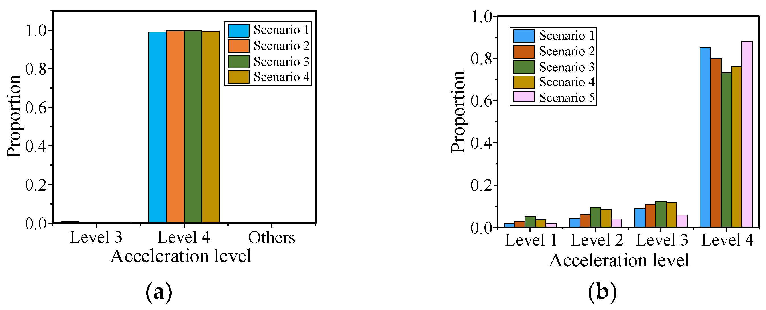
The analysis results for typical scenarios are shown in

Table 6. Statistical analysis of typical scenario clustering results.

Parameters	Classification	Scenario 1	Scenario 2	Scenario 3	Scenario 4
Speed (m/s)	Low speed	18.7%	30.4%	54.9%	16.8%
	Medium speed	24.8%	45.9%	35.3%	24.5%
	High speed	56.5%	19.7%	9.8%	58.7%
Acceleration (m/s2)	Level three	0.7%	0.3%	0.4%	0.4%
	Level four	99.1%	99.7%	99.6%	99.5%
	Others	0.2%	0	0	0.1%
	Average	−0.0597	−0.33	−0.3682	0.1243
	Standard deviation	0.3812	0.4521	0.3456	0.3449
Steering wheel angle (°)	Minimum average steering wheel angle	−0.7614	−5.1246	−17.9846	−2.8176
	Maximum average steering wheel angle	3.916	6.8848	27.9020	3.7130
The behavior of ego vehicle	Left lane changing (Turn left)	87.03%	73.55%	78.57%	88.25%
	Right lane changing (Turn right)	6.87%	15.79%	16.52%	5.25%
	Straight ahead	6.10%	10.66%	4.91%	6.50%
Target motion state	Uniform speed	35.5%	7.29%	4.83%	4.32%
	Deceleration	32.2%	81.51%	53.23%	48.87%
	Acceleration	32.75%	11.2%	41.94%	46.77%
Target position	Straight ahead	71.81%	82.05%	87.5%	76.67%
	Left cut in	16.70%	7.42%	4.46%	10.90%
	Right cut in	11.48%	10.53%	8.04%	12.43%
Types of surrounding traffic participants	Pedestrian	0.1%	0.5%	0.1%	1.6%
	Bicycle	0	0	0	0
	Light vehicle	95.7%	90.2%	95.4%	94.8%
	Heavy vehicle	2.7%	1.2%	0.5%	1.7%
	Tractor	0.1%	0.1%	0.1%	0.2%
Total	Numbers	1820	741	224	2799
	Proportion	32.6%	13.3%	4.0%	50.1%

. In this study, speeds below 11 m/s are considered as low, speeds between 11 m/s and 22 m/s as medium, and speeds above 22 m/s as high. According to the driver’s dangerous driving standard, the danger level can be divided into four categories. Level one is defined as an absolute acceleration value greater than or equal to 2.78 m/s², level two falls between 2.22 m/s² and 2.78 m/s², level three is between 1.67 m/s² and 2.22 m/s², while level four is less than 1.67 m/s². Level one and level two represent dangerous driving with sudden braking and acceleration, which may lead to safety accidents. Level three represents normal driving and braking with large amplitudes, and poses some risk. Level four represents normal driving with higher safety. It should be noted that both the first-level and second-level standards for acceleration are rarely presented in typical scenarios. Therefore, the first-level and second-level standards are denoted as ‘Others’.

From Table 6, each scenario includes two or more parameter variables for each element. For instance, the velocity element in the first category has three parameter variables: low speed, medium speed, and high speed. To address this issue, the scenario selection will be based on the element with the highest proportion of scenario element variables.

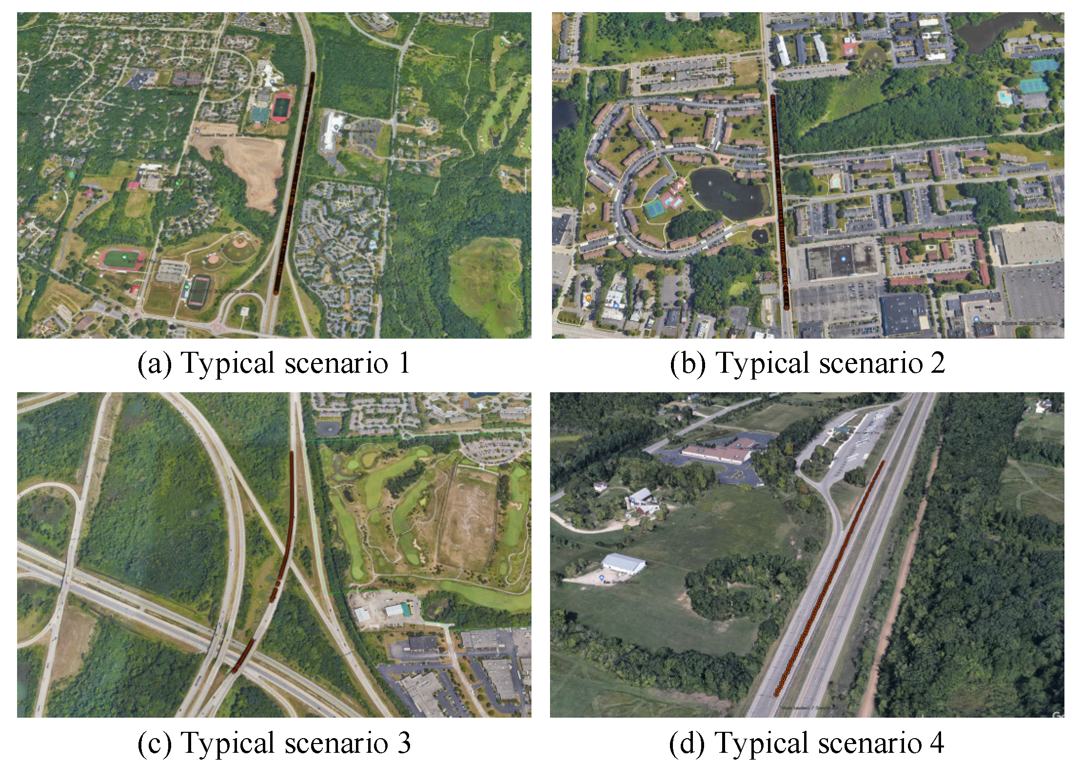
By applying Google Earth, the GPS data for each type of scene are projected in order to observe the road types and surrounding environmental conditions of the traveling vehicle. The driving environments of four typical scenes are identified as expressway, urban roads, suburbs, and expressway. Furthermore, multiple consecutive times from different scene categories are projected, as shown in Figure 11, where the red dot represents the vehicle’s position at each sampling moment. Upon observation, the road conditions for the four scenes are found to be as follows: straight road, straight road, curve road, and straight road.

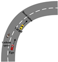
A summary of the four typical scene characteristic parameters is drawn up according to the analysis results mentioned above, and the results of this are shown in

Table 7. The results of typical scenario identification.

Parameters	Scenario 1	Scenario 2	Scenario 3	Scenario 4
Regional distribution	Expressway	City	Suburb	Expressway
Ego vehicle behavior	Straight ahead	Straight ahead	Driving around a curve	Straight ahead
Ego vehicle state	Uniform speed	Deceleration	Deceleration	Acceleration
Target type	Light vehicle	Light vehicle	Light vehicle	Light vehicle
Target state	Uniform speed	Deceleration	Deceleration	Acceleration
Target position	Straight ahead	Straight ahead	Driving around a curve	Straight ahead
Traffic flow	Vehicles on the right	Vehicles on both sides	Vehicles on the left	Vehicles on the left
Number of surrounding traffic participants	1–4	1–10	1–5	1–5
Intersection shape	Non-intersection	Non-intersection	Non-intersection	Non-intersection
Straight road/curved road	Straight road	Straight road	Curve road	Straight road
Diagram

. The four types of scenes are as follows: (1) scenario 1 depicts a high-speed, constant speed straight driving scenario, where the road environment consists of a high-speed section with fewer surrounding vehicles, and the target vehicle maintains a constant speed. (2) Scenario 2 represents medium-speed driving with vehicle deceleration, where the road environment is a straight urban road segment with a higher density of surrounding vehicles, and the target vehicle decelerates. (3) Scenario 3 involves low-speed driving with deceleration. In this example, the road environment is a suburban road with noticeable changes in steering angles, representing a typical scenario of deceleration in a curved road. The target vehicle slows down. (4) Scenario 4 features high-speed driving with slight acceleration and fewer surrounding vehicles. The target vehicle accelerates while driving on a straight high-speed road. Therefore, Scenario 4 is a typical high-speed acceleration scenario.

Analyzing extreme scenarios using the same method yields the results shown in

Table 8. Statistical analysis of extreme scenario clustering results.

Parameters	Classification	Scenario 1	Scenario 2	Scenario 3	Scenario 4	Scenario 5
Speed (m/s)	Low speed	22.4%	62.6%	53.6%	30.9%	66.7%
	Medium speed	25.2%	23.0%	19.9%	33.3%	29.4%
	High speed	52.4%	11.4%	27.5%	35.8%	3.9%
Acceleration (m/s2)	Level one	1.8%	2.9%	5.0%	3.6%	2.0%
	Level two	4.2%	6.3%	9.5%	8.5%	3.9%
	Level three	8.9%	10.9%	12.3%	11.7%	5.9%
	Level four	85.1%	79.9%	73.2%	76.2%	88.2%
	Average	−0.026	−0.046	0.065	−0.0223	−0.146
	Standard deviation	0.5836	0.8203	0.7697	0.7015	0.8583
Steering wheel angle	Minimum average steering wheel angle	−13.179	−47.258	−42.187	−16.275	−66.347
	Maximum average steering wheel angle	21.133	53.7619	39.187	21.405	34.264
The behavior of ego vehicle	Left lane changing (Turn left)	11.90%	25.29%	20.67%	9.02%	64.71%
	Right lane changing (Turn right)	16.87%	41.95%	16.20%	18.03%	29.41%
	Straight ahead	71.23%	32.76%	63.13%	72.95%	5.88%
Target motion state	Uniform speed	35.91%	10.92%	62.01%	31.97%	41.18%
	Deceleration	62.30%	61.49%	19.55%	63.93%	54.90%
	Acceleration	1.79%	27.59%	18.44%	4.10%	3.92%
Target position	Straight ahead	69.64%	38.51%	54.19%	52.73%	100%
	Left cut in	15.48%	49.43%	30.73%	18.58%	0
	Right cut in	14.88%	12.06%	15.08%	28.69%	0
Types of surrounding traffic participants	Pedestrian	0.1%	0.04%	0.4%	0.2%	0.7%
	Bicycle	0	0	0	0	0
	Light vehicle	84.9%	72.1%	81.6%	83.6%	72.8%
	Heavy vehicle	2.5%	0.8%	2.4%	2.4%	1.1%
	Tractor	0.4%	0	0.5%	0.9%	0
Total	Numbers	504	174	179	366	51
	Proportion	39.5%	13.7%	14.1%	28.7%	4%

.

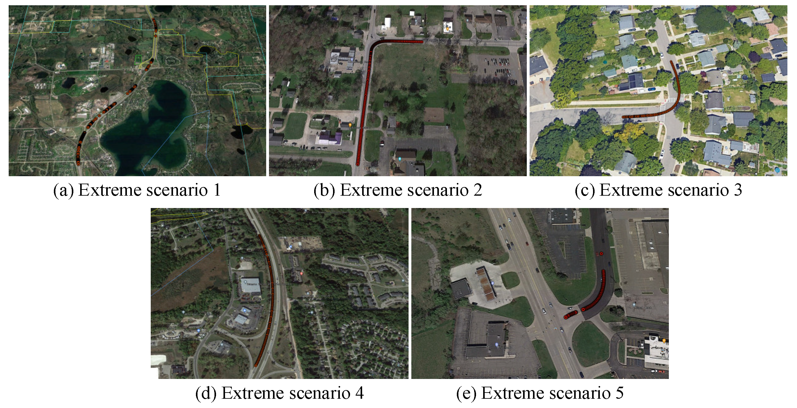
Applying Google Earth to project GPS data of each type of extreme scenario, as shown in Figure 12, the driving environments for the five typical scenarios are identified as expressway, urban road, urban road, expressway, and urban road. The road conditions for the five scenarios are continuous curves, intersection, intersection, curves, and intersection.

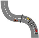
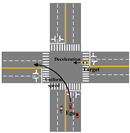
The five types of extreme testing scenarios are extracted, and the characteristics and parameter features of extreme scenarios are summarized, based on the analysis results of the extreme scenarios mentioned above, as shown in

Table 9. The results of extreme scenario identification.

Parameters	Scenario 1	Scenario 2	Scenario 3	Scenario 4	Scenario 5
Regional distribution	Expressway	City	City	Expressway	City
Ego vehicle behavior	Driving around a curve	Turn right	Turn left	Driving around a curve	Turn left
Ego vehicle state	Uniform speed	Uniform speed	Uniform speed	Uniform speed	Deceleration
Target type	Light vehicle	Light vehicle	Light vehicle	Light vehicle	Light vehicle
Target state	Deceleration	Deceleration	Deceleration	Deceleration	Deceleration
Target position	Driving around a curve	Left cut in	Straight ahead	Driving around a curve	Straight ahead
Traffic flow	Vehicles on the left	Vehicles on both sides	Vehicles on both sides	Vehicles on the left	Vehicles on both sides
Number of surrounding traffic participants	1–9	1–12	1–11	1–10	1–8
Intersection shape	Non-intersection	Intersection	Intersection	Non-intersection	Intersection
Straight road/curved road	Curve road	Straight road	Straight road	Curve road	Straight road
Diagram

.

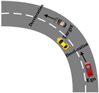
In extreme scenario 1, the vehicle is continuously turning while traveling at a high speed, and there is another vehicle ahead with a decreasing relative velocity, posing a safety hazard. In extreme scenario 2, the vehicle is approaching an intersection with complex road conditions and heavy traffic. The vehicle tends to make a right turn, and there is a risk of conflict and collision with other vehicles merging into the main lane. In extreme scenario 3, the vehicle is approaching an intersection with complex road conditions and heavy traffic. The vehicle tends to make a left turn, and there is a risk of conflict and collision with other vehicles on intersecting paths. In extreme scenario 4, the main vehicle is traveling at high speed on a curved road with other vehicles ahead, increasing the risk of driving. In extreme scenario 5, the vehicle is approaching an intersection with complex road conditions and heavy traffic. The vehicle tends to make a left turn, and there is a risk of conflict and collision with other vehicles on intersecting paths.

4.4. Comparative Analysis of Typical-Extreme Scenarios

As shown in Figure 13, the proportions of acceleration levels one, two, and three in extreme scenarios are significantly higher compared to typical scenarios. This indicates that in these five scenarios, the incidence of dangerous driving conditions such as sudden deceleration and rapid acceleration is noticeably increased. Additionally, in extreme scenarios, vehicles operate in complex environments such as intersections and curves with a higher number of surrounding vehicles. These factors collectively increase the driving risk.

5. Conclusions

This paper proposes an automatic driving test scenario identification method based on deep unsupervised learning that combines IF, 1D-RCAE, and IE-improved K-means algorithms. Firstly, data variables that can represent the ego vehicle state and surrounding environment information are selected as the segmentation criteria. IF is employed for typical–extreme scenario segmentation, and the results demonstrate that IF can obtain more interpretable segmentation results compared to LOF and OCSVM. Secondly, a novel network called 1D-RCAE is designed to extract scene features. The results illustrate that the 1D-RCAE outperforms other networks, highlighting its superior feature extraction capability. Finally, considering the different importance of different features, the K-means algorithm is optimized using IE, and the extracted scene features are clustered. By analyzing the characteristics of each scene parameter in different categories, four typical scenes and five extreme scenes are obtained. The IE-optimized K-means algorithm is compared with other commonly applied clustering algorithms, and the results demonstrate that the performance of the IE-improved K-means algorithm outperforms those of other algorithms. The identified scenes can provide strong support for the construction of an automatic driving test scenario library.

In the future, virtual test scenarios will be constructed based on the identified scenes to test the autonomous driving systems, and an assessment system will be built to evaluate the test results quantitatively and provide suggestions of how to optimize the autonomous driving systems. Additionally, based on this foundation, research will be also conducted on scene generalization to generate various types of scenarios, enriching the automated driving test scenario library. These scenarios will be applied for automated driving algorithm verification, identifying deficiencies through scenario testing and making improvements in order to enhance the safety of autonomous vehicles.

References

1. Li, Z.; Huang, X.; Wang, J.; Mu, T. Lane Change Behavior Research Based on NGSIM Vehicle Trajectory Data. In Proceedings of the 2020 Chinese Control And Decision Conference (CCDC), Hefei, China, 22–24 August 2020; pp. 1865–1870. [Google Scholar]
2. Zhai, M.; Xiang, X.; Lv, N.; Saddik, A.E. Multi-Task Learning in Autonomous Driving Scenarios Via Adaptive Feature Refinement Networks. In Proceedings of the ICASSP 2020—2020 IEEE International Conference on Acoustics, Speech and Signal Processing (ICASSP), Barcelona, Spain, 4–8 May 2020; pp. 2323–2327. [Google Scholar]
3. Krajewski, R.; Bock, J.; Kloeker, L.; Eckstein, L. The highD Dataset: A Drone Dataset of Naturalistic Vehicle Trajectories on German Highways for Validation of Highly Automated Driving Systems. In Proceedings of the 2018 21st International Conference on Intelligent Transportation Systems (ITSC), Maui, HI, USA, 4–7 November 2018; pp. 2118–2125. [Google Scholar]
4. Gu, J.; Zhao, H.; Lin, Z.; Li, S.; Cai, J.; Ling, M. Scene Graph Generation With External Knowledge and Image Reconstruction. In Proceedings of the 2019 IEEE/CVF Conference on Computer Vision and Pattern Recognition (CVPR), Long Beach, CA, USA, 15–20 June 2019; pp. 1969–1978. [Google Scholar]
5. Ries, L.; Langner, J.; Otten, S.; Bach, J.; Sax, E. A Driving Scenario Representation for Scalable Real-Data Analytics with Neural Networks. In Proceedings of the 2019 IEEE Intelligent Vehicles Symposium (IV), Paris, France, 9–12 June 2019; pp. 2215–2222. [Google Scholar]
6. Du, Z.; Zhang, L.; Zhao, S.; Hou, Q.; Zhai, Y. Research on Test and Evaluation Method of L3 Intelligent Vehicle Based on Chinese Characteristics Scene. In Proceedings of the 2020 IEEE 4th Information Technology, Networking, Electronic and Automation Control Conference (ITNEC), Chongqing, China, 12–14 June 2020; pp. 26–32. [Google Scholar]
7. Ding, W.; Xu, M.; Zhao, D. CMTS: A Conditional Multiple Trajectory Synthesizer for Generating Safety-Critical Driving Scenarios. In Proceedings of the 2020 IEEE International Conference on Robotics and Automation (ICRA), Paris, France, 31 May–31 August 2020; pp. 4314–4321. [Google Scholar]
8. Hou, L.; Xin, L.; Li, S.E.; Cheng, B.; Wang, W. Interactive Trajectory Prediction of Surrounding Road Users for Autonomous Driving Using Structural-LSTM Network. IEEE Trans. Intell. Transp. Syst. 2020, 21, 4615–4625. [Google Scholar] [CrossRef]
9. Li, X.S.; Cui, X.T.; Ren, Y.Y.; Zheng, X.L. Unsupervised Driving Style Analysis Based on Driving Maneuver Intensity. IEEE Access 2022, 10, 48160–48178. [Google Scholar] [CrossRef]
10. Pang, M.Y. Trajectory Data Based Clustering and Feature Analysis of Vehicle Lane-Changing Behavior. In Proceedings of the 2019 4th International Conference on Electromechanical Control Technology and Transportation (ICECTT), Guilin, China, 26–28 April 2019; pp. 229–233. [Google Scholar]
11. Ren, Y.Y.; Zhao, L.; Zheng, X.L.; Li, X.S. A Method for Predicting Diverse Lane-Changing Trajectories of Surrounding Vehicles Based on Early Detection of Lane Change. IEEE Access 2022, 10, 17451–17472. [Google Scholar] [CrossRef]
12. Wang, Z.; Ma, X.; Liu, J.; Chigan, D.; Liu, G.; Zhao, C. Car-Following Behavior of Coach Bus Based on Naturalistic Driving Experiments in Urban Roads. In Proceedings of the 2019 IEEE International Symposium on Circuits and Systems (ISCAS), Sapporo, Japan, 26–29 May 2019; pp. 1–4. [Google Scholar]
13. Masmoudi, M.; Friji, H.; Ghazzai, H.; Massoud, Y. A Reinforcement Learning Framework for Video Frame-Based Autonomous Car-Following. IEEE Open J. Intell. Transp. Syst. 2021, 2, 111–127. [Google Scholar] [CrossRef]
14. Zhao, D.; Guo, Y.; Jia, Y.J. TrafficNet: An open naturalistic driving scenario library. In Proceedings of the 2017 IEEE 20th International Conference on Intelligent Transportation Systems (ITSC), Yokohama, Japan, 16–19 October 2017; pp. 1–8. [Google Scholar]
15. Martinsson, J.; Mohammadiha, N.; Schliep, A. Clustering Vehicle Maneuver Trajectories Using Mixtures of Hidden Markov Models. In Proceedings of the 2018 21st International Conference on Intelligent Transportation Systems (ITSC), Maui, HI, USA, 4–7 November 2018; pp. 3698–3705. [Google Scholar]
16. Wang, W.; Ramesh, A.; Zhu, J.; Li, J.; Zhao, D. Clustering of Driving Encounter Scenarios Using Connected Vehicle Trajectories. IEEE Trans. Intell. Veh. 2020, 5, 485–496. [Google Scholar] [CrossRef] [Green Version]
17. Wang, W.; Zhao, D. Extracting Traffic Primitives Directly From Naturalistically Logged Data for Self-Driving Applications. IEEE Rob. Autom. Lett. 2018, 3, 1223–1229. [Google Scholar] [CrossRef] [Green Version]
18. Zhao, J.; Fang, J.; Ye, Z.; Zhang, L. Large Scale Autonomous Driving Scenarios Clustering with Self-supervised Feature Extraction. In Proceedings of the 2021 IEEE Intelligent Vehicles Symposium (IV), Nagoya, Japan, 11–17 July 2021; pp. 473–480. [Google Scholar]
19. Zhao, S.; Wu, Y.; Zhu, X.; Zhou, B.; Bao, H.; Zhang, L. Research on Automatic Classification for Driving Scenarios Based on Big Data and Ontology. In Proceedings of the 2018 IEEE 4th International Conference on Computer and Communications (ICCC), Chengdu, China, 7–10 December 2018; pp. 1857–1862. [Google Scholar]
20. Xiaoyu, S.; Xichan, Z.; Kaiyuan, Z.; Lin, L.; Zhixiong, M.; Dazhi, W. Automatic detection method research of incidents in China-FOT database. In Proceedings of the 2016 IEEE 19th International Conference on Intelligent Transportation Systems (ITSC), Rio de Janeiro, Brazil, 1–4 November 2016; pp. 754–759. [Google Scholar]
21. Wachenfeld, W.; Junietz, P.; Wenzel, R.; Winner, H. The worst-time-to-collision metric for situation identification. In Proceedings of the 2016 IEEE Intelligent Vehicles Symposium (IV), Gothenburg, Sweden, 19–22 June 2016; pp. 729–734. [Google Scholar]
22. Tan, S.; Wong, K.; Wang, S.; Manivasagam, S.; Ren, M.; Urtasun, R. SceneGen: Learning to Generate Realistic Traffic Scenes. In Proceedings of the 2021 IEEE/CVF Conference on Computer Vision and Pattern Recognition (CVPR), Nashville, TN, USA, 20–25 June 2021; pp. 892–901. [Google Scholar]
23. Rocklage, E.; Kraft, H.; Karatas, A.; Seewig, J. Automated scenario generation for regression testing of autonomous vehicles. In Proceedings of the 2017 IEEE 20th International Conference on Intelligent Transportation Systems (ITSC), Yokohama, Japan, 16–19 October 2017; pp. 476–483. [Google Scholar]
24. Fellner, A.; Krenn, W.; Schlick, R.; Tarrach, T.; Weissenbacher, G. Model-based, Mutation-driven Test-case Generation Via Heuristic-guided Branching Search. ACM Trans. Embedded Comput. Syst. 2019, 18, 1–28. [Google Scholar] [CrossRef] [Green Version]
25. Spooner, J.; Palade, V.; Cheah, M.; Kanarachos, S.; Daneshkhah, A. Generation of Pedestrian Crossing Scenarios Using Ped-Cross Generative Adversarial Network. Appl. Sci. 2021, 11, 471. [Google Scholar] [CrossRef]
26. Feng, S.; Feng, Y.; Yu, C.; Zhang, Y.; Liu, H.X. Testing Scenario Library Generation for Connected and Automated Vehicles, Part I: Methodology. IEEE Trans. Intell. Transp. Syst. 2021, 22, 1573–1582. [Google Scholar] [CrossRef] [Green Version]
27. Koren, M.; Alsaif, S.; Lee, R.; Kochenderfer, M.J. Adaptive Stress Testing for Autonomous Vehicles. In Proceedings of the 2018 IEEE Intelligent Vehicles Symposium (IV), Changshu, China, 26–30 June 2018; pp. 1–7. [Google Scholar]
28. Zhang, L.; Liu, L. Data Anomaly Detection Based on Isolation Forest Algorithm. In Proceedings of the 2022 International Conference on Computation, Big-Data and Engineering (ICCBE), Yunlin, Taiwan, 27–29 May 2022; pp. 87–89. [Google Scholar]
29. Liu, H.; Taniguchi, T.; Tanaka, Y.; Takenaka, K.; Bando, T. Visualization of Driving Behavior Based on Hidden Feature Extraction by Using Deep Learning. IEEE Trans. Intell. Transp. Syst. 2017, 18, 2477–2489. [Google Scholar] [CrossRef]
30. He, K.; Zhang, X.; Ren, S.; Sun, J. Deep Residual Learning for Image Recognition. In Proceedings of the 2016 IEEE Conference on Computer Vision and Pattern Recognition (CVPR), Las Vegas, NV, USA, 27–30 June 2016; pp. 770–778. [Google Scholar]
31. Szegedy, C.; Ioffe, S.; Vanhoucke, V.; Alemi, A. Inception-v4, Inception-ResNet and the Impact of Residual Connections on Learning. AAAI Conf. Artif. Intell. 2016, 31, 1. [Google Scholar] [CrossRef]
32. Xie, S.; Girshick, R.; Dollár, P.; Tu, Z.; He, K. Aggregated Residual Transformations for Deep Neural Networks. In Proceedings of the 2017 IEEE Conference on Computer Vision and Pattern Recognition (CVPR), Honolulu, HI, USA, 21–26 July 2017; pp. 5987–5995. [Google Scholar]
33. Ioffe, S.; Szegedy, C. Batch Normalization: Accelerating Deep Network Training by Reducing Internal Covariate Shift. arXiv 2015, arXiv:1502.03167. [Google Scholar]
34. Xingxing, L.; Changjun, F.; Baoxin, X.; Chao, C. Evaluation algorithm for clustering quality based on information entropy. In Proceedings of the 2016 IEEE International Conference on Big Data Analysis (ICBDA), Hangzhou, China, 12–14 March 2016; pp. 1–5. [Google Scholar]
35. Wang, W.; Liu, C.; Zhao, D. How Much Data Are Enough? A Statistical Approach With Case Study on Longitudinal Driving Behavior. IEEE Trans. Intell. Veh. 2017, 2, 85–98. [Google Scholar] [CrossRef] [Green Version]
36. Liu, J.; Khattak, A. Delivering improved alerts, warnings, and control assistance using basic safety messages transmitted between connected vehicles. Transp. Res. Part C Emerg. Technol. 2016, 68, 83–100. [Google Scholar] [CrossRef]
37. Zhang, C.; Zhang, H.; Sun, G.; Ma, X. Transformer Anomaly Detection Method Based on MDS and LOF Algorithm. In Proceedings of the 2022 7th Asia Conference on Power and Electrical Engineering (ACPEE), Hangzhou, China, 15–17 April 2022; pp. 987–991. [Google Scholar]
38. Minjie, Z.; Yilian, Z. Abnormal Traffic Detection Technology of Power IOT Terminal Based on PCA and OCSVM. In Proceedings of the 2023 IEEE 6th Information Technology, Networking, Electronic and Automation Control Conference (ITNEC), Chongqing, China, 24–26 February 2023; pp. 549–553. [Google Scholar]
39. Gupta, T.; Panda, S.P. Clustering Validation of CLARA and K-Means Using Silhouette & DUNN Measures on Iris Dataset. In Proceedings of the 2019 International Conference on Machine Learning, Big Data, Cloud and Parallel Computing (COMITCon), Faridabad, India, 14–16 February 2019; pp. 10–13. [Google Scholar]
40. Aguilar, J.; Gull, C.Q.; Moreno, M.D.R.; Viera, J. Analysis of Customer Energy Consumption Patterns using an Online Fuzzy Clustering Technique. In Proceedings of the 2022 IEEE International Conference on Fuzzy Systems (FUZZ-IEEE), Padua, Italy, 18–23 July 2022; pp. 1–6. [Google Scholar]
41. Gonzales, M.E.M.; Uy, L.C.; Sy, J.A.L.; Cordel, M.O. Distance Metric Recommendation for k-Means Clustering: A Meta-Learning Approach. In Proceedings of the TENCON 2022—2022 IEEE Region 10 Conference (TENCON), Hong Kong, China, 1–4 November 2022; pp. 1–6. [Google Scholar]
Figure 1. The research framework overview of this paper.
Wevj 14 00208 g001
Figure 2. The flow chart of the proposed methodology.
Wevj 14 00208 g002
Figure 3. Residual module diagram.
Wevj 14 00208 g003
Figure 4. 1D-RCAE feature extraction model.
Wevj 14 00208 g004
Figure 5. The network structure of 1D-RCAE.
Wevj 14 00208 g005
Figure 6. Segmentation results of velocity and acceleration. (a) Velocity segmentation result; (b) acceleration segmentation result.
Wevj 14 00208 g006
Figure 7. Comparison of segmentation results from different algorithms.
Wevj 14 00208 g007
Figure 8. Loss values. (a) Training loss and validation loss of the 1D-RCAE; (b) comparison of training losses between CAE and 1D-RCAE.
Wevj 14 00208 g008
Figure 9. Elbow plots of typical scenario and extreme scenario. (a) Typical scenarios; (b) extreme scenario.
Wevj 14 00208 g009
Figure 10. Comparison of different networks.
Wevj 14 00208 g010
Figure 11. Typical scenario projection.
Wevj 14 00208 g011
Figure 12. Extreme scenario projection.
Wevj 14 00208 g012
Figure 13. Distribution of acceleration levels in typical scenarios and extreme scenarios. (a) Typical scenarios; (b) extreme scenarios.
Wevj 14 00208 g013