Abstract
Aiming at the problem that, under certain extreme conditions, relying on tire force or tire angular velocity to represent the longitudinal velocity of the unmanned vehicle will fail, this paper proposes a longitudinal velocity estimation method that fuses LiDAR and inertial measurement unit (IMU). First, in order to improve the accuracy of LiDAR odometry, IMU information is introduced in the process of eliminating point cloud motion distortion. Then, the statistical characteristic of the system noise is tracked by an adaptive noise estimator, which reduces the model error and suppresses the filtering divergence, thereby improving the robustness and filtering accuracy of the algorithm. Next, in order to further improve the estimation accuracy of longitudinal velocity, time-series analysis is used to predict longitudinal acceleration, which improves the accuracy of the prediction step in the unscented Kalman filter (UKF). Finally, the feasibility of the estimation method is verified by simulation experiments and real-vehicle experiments. In the simulation experiments, medium- and high-velocity conditions are tested. In high-velocity conditions (0–30 m/s), the average error is 1.573 m/s; in the experiment, the average error is 0.113 m/s.
1. Introduction
Longitudinal velocity is the velocity component along the forward direction of the vehicle body during driving, and its estimation accuracy directly affects the safety control of the vehicle by active and passive safety systems such as the anti-lock braking system and acceleration slip regulation [1,2]. Low-precision longitudinal velocity estimation not only increases unnecessary energy consumption, but may even affect the safety of passengers. Therefore, in order to achieve high-precision control of driverless vehicles, reduce energy consumption, and ensure the safety of passengers, it is of great significance to carry out in-depth research on vehicle longitudinal velocity estimation methods in the field of driverless vehicles [3].
Research on vehicle longitudinal velocity estimation methods can be divided into two directions: dynamics-based methods and kinematics-based methods [4], as well as some intelligent estimation methods [5,6,7]. The dynamics-based method mainly relies on the dynamics model of the vehicle, and it estimates the longitudinal velocity of the vehicle by analyzing the force of the vehicle model. In [8], a nonlinear dynamic model including the longitudinal velocity, lateral velocity and yaw rate of the vehicle was established based on the linear tire model, and the real-time estimation of the vehicle velocity was realized. In [9], a nonlinear dynamic model including longitudinal velocity, lateral velocity, yaw angular velocity and four-wheel angular velocities was established based on the tire model of magic formula, and the vehicle velocity was estimated by using the unscented Kalman filter (UKF). In [10], a hybrid Kalman filter was proposed. When the system noise statistical characteristic error is small, the square root cubature Kalman filter is used to estimate the vehicle velocity; when the system noise statistical characteristic error is large, the square root cubature Kalman finite impulse filter is used for real-time estimation of the vehicle velocity. In [11], a state estimation method based on IMU is proposed, which uses two estimators based on the vehicle dynamics model to estimate longitudinal speed, pitch angle, lateral speed, and roll angle.
However, the dynamics-based method is less affected by external environmental factors, and it is limited by the dynamics model; the accuracy of the estimation algorithm cannot be guaranteed in some extreme conditions. Therefore, this paper mainly studies the kinematics-based estimation method. In [12], improvements have been made to the system noise of the UKF to prevent filtering divergence. In [13], the sideslip angle of the vehicle’s center of mass was described by using the vehicle yaw rate, longitudinal velocity, and lateral acceleration, and then the vehicle’s lateral velocity was deduced by using the definition formula of the vehicle’s center of mass sideslip angle. In [14], the vehicle yaw rate was taken as the scheduling parameter, a linear time-varying parameter vehicle kinematics model was established, and the real-time estimation of the vehicle velocity was realized by using the robust filter. In [15,16], a kinematics model was established including the longitudinal and lateral velocities of the vehicle using the tire longitudinal and lateral forces measured by the sensor, and real-time estimation of the longitudinal and lateral velocities of the vehicle was realized by using the Kalman filter. In [17], the tire lateral force measured by the sensor in a hybrid nominal model was established including the kinematics and dynamics of the vehicle, and the real-time estimation of the vehicle velocity was realized by using the extended Kalman filter. In [15,16,17], the tire force was considered measurable state information, but in view of the assembly position of the tire force sensor and the constraints of the use condition, it is difficult to meet the control requirements of driverless vehicles.
This problem can be solved by combining positioning technology and IMU to estimate the velocity of the vehicle. Usually, the combination of GPS and IMU can be used to obtain accurate estimation results [18]. In [19], the accuracy of estimated heading and position was improved by using carrier-phase differential GPS. In [20], the lateral velocity is estimated by using two low-cost GPS, and the problem of low frequency of traditional GPS signals is compensated by combining with IMU. In [21], an extended square-root cubic Kalman filter was proposed to combine GPS and IMU. In [22], motion and constraint models were combined with IMU data to overcome interference from gyroscope drift and disturbances in external acceleration. In [23], a novel Kalman filter is proposed to solve the problem of sensor jitter noise, which further improves the estimation accuracy. However, GPS may lose signal in some areas, resulting in serious estimation errors [24]. Meanwhile, with the development of autonomous driving technology, high-precision and highly robust autonomous vehicle positioning technology is one of the fundamental technologies in the field of autonomous driving. However, the above research results have not fully utilized the positioning information of driverless vehicles for velocity estimation.
Therefore, this paper proposes a method that integrates LiDAR and IMU information to achieve accurate estimation of longitudinal velocity, which addresses the issues of relying on tires to indicate the failure of vehicle longitudinal velocity under certain extreme operating conditions and the possibility of GPS losing signal in certain areas. At the same time, in order to reduce model error and suppress filtering divergence, a noise adaptive module (AUKF) is added to the UKF, and time-series analysis is introduced into the adaptive unscented Kalman filter (TSA-AUKF) to further improve estimation accuracy. The structure of the proposed method is shown in Figure 1. Based on this, the novelties of this paper are summarized as follows:
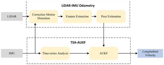
Figure 1.
The structure of the longitudinal velocity estimation method.
- To address the issue of point cloud distortion during the motion of LiDAR, IMU is used to predict the pose changes of LiDAR to reduce the impact of motion distortion on odometry accuracy.
- Time-series analysis is introduced into the motion equation to predict the trend of longitudinal acceleration changes through multiple sets of IMU historical data, thereby improving the estimation accuracy of the filtering algorithm.
The rest of this paper is structured as follows. In the second section, the LiDAR-IMU odometry is introduced. In the third section, the proposed longitudinal velocity estimation method is introduced. In the fourth section, simulation experiments and real vehicle experiments are conducted, and the results are analyzed. In the fifth section, the full text is summarized.
2. LiDAR-IMU Odometry
2.1. Correction of Point Cloud Motion Distortion
This paper uses a mechanical rotating LiDAR to output a point cloud collected within a cycle as one frame. When the system is in motion and the position of the LiDAR changes, the point cloud within a frame corresponds to different coordinate origins, resulting in motion distortion of the obtained point cloud data, as shown in Figure 2.
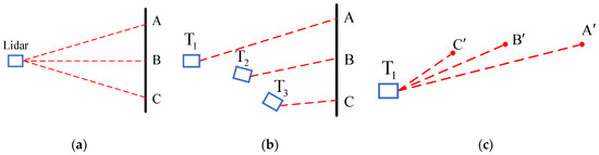
Figure 2.
The principle of motion distortion generation: (a) LiDAR scanning starting point; (b) LiDAR motion process; (c) Point cloud distortion caused by motion.
In order to correct the motion distortion of LiDAR, it is necessary to obtain the pose changes of LiDAR within one frame. However, due to the fact that LiDAR is often in variable velocity motion and the low update frequency of LiDAR odometry, the actual application effect is poor. The IMU sampling frequency can reach 100 Hz, which can accurately reflect the movement and high-precision local pose estimation. By integrating the data collected by IMU and using linear interpolation, the pose increment of the laser point at any time relative to time can be obtained. The calculation formula is
The laser point coordinates at time are converted to the first laser point coordinate system through pose increment. The calculation formula is
where is the position of the laser point at time , and is the position of in the coordinate system of the first laser point. The use of IMU to eliminate motion distortion in LiDAR can effectively avoid problems such as map ghosting caused by distortion. The effect of motion distortion removal is shown in Figure 3.
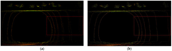
Figure 3.
The comparison of motion distortion removal: (a) The point cloud of the same laser beam in the red box cannot be aligned before removing motion distortion; (b) Aligning point cloud of the same laser beam after distortion removal.
2.2. LiDAR Point Cloud Clustering
During the information collection process of LiDAR, small objects may not repeatedly appear in adjacent frames, causing errors in inter-frame matching. Therefore, this paper calculates the angle between adjacent laser beam scanning points and point cloud clusters based on the size of the angle. If the clustering results are less than 30 points, they are removed as noise points to improve feature extraction accuracy and inter-frame matching efficiency. As shown in Figure 4, traverse from the red point as the center to adjacent points (green points) around, calculate the angle between the center point and adjacent points , until the clustering conditions are not met.
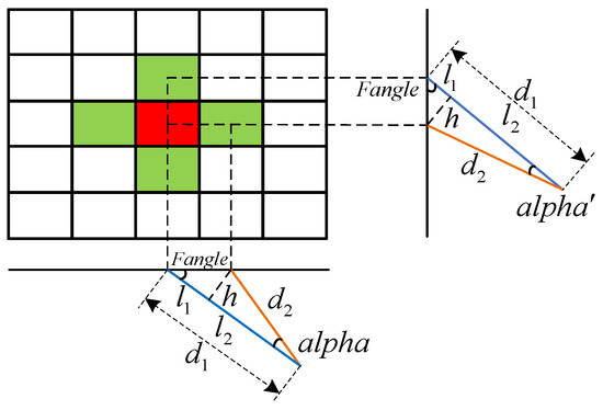
Figure 4.
Flatness-based clustering analysis.
The calculation process is
Flatness is
where and are the lengths of blue and orange laser beams, and and are the angular resolutions in the horizontal and vertical directions, respectively. When adjacent laser beam scanning points are on the same horizontal line, is equal to the horizontal angular resolution . When adjacent laser beam scanning points are on the same vertical line, is equal to the vertical angular resolution . During the iteration process, points with flatness greater than the threshold are placed in set . When the number of points in set is less than 30 at the end of the iteration, points in set are removed as noise points.
2.3. Feature Extraction of Point Cloud
After clustering the original point cloud of the LiDAR, the distance image is horizontally divided into several sub-images, and each sub-image is traversed and processed sequentially. Any point is selected in the point cloud, multiple continuous points in the vertical direction of point are selected to construct a point set , and the smoothness of each point in the point set is calculated as
By setting threshold to distinguish the features of points, those with smoothness greater than the threshold are edge points, while those with smoothness greater than the threshold are planar points. To evenly extract features from all directions, the LiDAR scanning data are divided into two subsets horizontally. The smoothness of the points in the subset is sorted, and the edge feature point with the highest roughness is selected from each row of the subset. Then, the planar feature point with the lowest roughness is selected in the same way.
2.4. Feature Matching of Point Cloud
By extracting the feature points of the LiDAR keyframe and matching the feature points of adjacent keyframes, the pose transformation relationship of the LiDAR can be solved. The point clouds scanned by the LiDAR at time and time are set as and , the edge feature point sets extracted from the feature extraction as and , and the planar feature point sets as and . The purpose of inter-frame matching is to obtain the transformation relationship between and , as well as the transformation relationship between and and the transformation relationship between and . Due to the distortion generated during the LiDAR motion process, the edge feature point set and planar feature point set extracted at time are projected to time , denoted as and . Edge points are points in sharp positions in a 3D environment, and edge feature points use a point-to-line matching method. Planar points are points located in a smooth region in a 3D environment, and planar feature points use point-to-face matching.
2.4.1. Edge Point Matching
A point in the set of edge feature points is selected at time , and the closest point to and the closest point in the scan line adjacent to point at time are selected, with coordinates , , and , as shown in Figure 5. The distance from point to line is
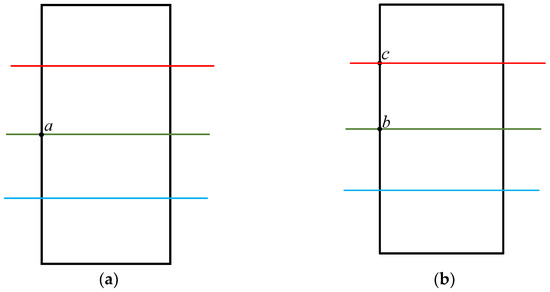
Figure 5.
Edge point feature matching: (a) Edge feature point set at time ; (b) Edge feature point set at time .
2.4.2. Planar Point Matching
A point in the set of planar feature points at time is selected, the closest point to at time is selected, and the closest point to in the same vertical resolution point set is found, as well as the closest point in the adjacent scanning laser line with point , with coordinates , , , and , as shown in Figure 6.
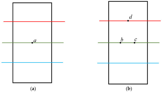
Figure 6.
Planar point feature matching; (a) Planar feature point set at time ; (b) Planar feature point set at time .
The distance from point to plane is
2.5. Pose Estimation
After matching the features of edge points and planar points, the point-to-line distance and point-to-planar distance are obtained. To obtain the optimal pose, the following cost function can be established by combining (8) and (9):
The error function is established by using the Lewinberg-Marquardt (L-M) method to optimize the solution:
where is the trust radius, and is the coefficient matrix. Constructing Lagrangian function:
where Is the coefficient. Simplify and derive (12) to obtain
Substituting (13) into equation (10) yields
where the coefficient matrix can be approximated as , so under the premise that the initial Jacobian matrix is known, the residual can be solved. Substitute the gradient descent formula as
Using two L-M optimization iterations to solve until convergence, obtain the pose transformation matrix . Finally, take the differential value of as a rough estimation of longitudinal velocity .
3. Fusion Method of LiDAR and IMU
3.1. AUKF
The nonlinear system of vehicle motion is
where and represent the motion state variables at time and , respectively, represents the motion model transfer matrix, represents process noise, represents the observation at time , represents the observation model transfer matrix, and represents the observation noise.
Set the initial estimation value and error covariance for the motion state:
At the same time, calculate the Sigma sampling points for the motion state:
where represents the dimension of , and represents the scaling factor, taken as .
Sigma sampling points are mapped through the motion model transfer matrix :
Then, perform weighted calculations to obtain the prediction and error covariance matrix of the motion state variables at time :
where represents the weight
Calculate the Sigma sampling points for the observed value as
where . Sigma sampling points are mapped through the motion model transfer matrix :
Then, perform weighted calculations to obtain the prediction and error covariance matrix of the observed value at time , as well as the cross-covariance matrix of the observation prediction error:
The Kalman gain can be calculated as
Finally, the motion state at time can be obtained as
Modeling error is an important component of process noise. By adaptively adjusting the covariance matrix of process noise based on the difference between observed and predicted values, estimation error can be reduced and filtering divergence can be suppressed. So, the difference between the observed and predicted values is defined as
where is affected by modeling errors and initial conditions, and the noise covariance matrix can be estimated based on . So, the theoretical covariance matrix of is
Due to the influence of modeling errors and observation noise, the actual value of the covariance matrix of often deviates from the theoretical value. So, the actual covariance matrix calculation method for is
where is the length of the sliding window.
is adjusted by comparing the actual covariance matrix of with the theoretical covariance matrix . is reduced when ; when is used, theoretically should be added, but to avoid filter divergence, can be kept constant. Define the adjustment factor as
In order to improve the estimation accuracy of the Kalman filter, the observation noise covariance matrix and the process noise covariance matrix are generally adjusted in the opposite direction [25]. Therefore, the adaptive adjustment method for the covariance matrix of state estimation error is
3.2. Longitudinal Acceleration Prediction
Due to the existence of (20), it is necessary to predict acceleration, but the acceleration of the vehicle is related to driver habits and current road conditions, making it difficult to describe it in mathematical language. Therefore, the ARIMA model in time-series analysis was used to predict the longitudinal acceleration of vehicles.
The essence of the ARIMA model is to achieve short-term prediction through historical observation data with sampling intervals and historical random interference with sampling intervals. Its mathematical expression is
where represents the order of the AR model; represents the order of the MA model; represents predicted data; , , and represent historical observation data; , , , and represent the AR model coefficients; , , and represent historical noise interference; ; , , and represent the coefficients of the MA model.
We used ten longitudinal acceleration datasets as a set of historical data and predicted the acceleration value at the next moment using ARIMA. The predicted and true values of longitudinal acceleration are shown in Figure 7, indicating that ARIMA has a certain predictive ability for longitudinal acceleration.
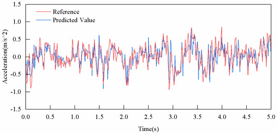
Figure 7.
Comparison between predicted and true values of longitudinal acceleration.
From (38), the predicted longitudinal acceleration at time can be obtained. However, observing (20), it is found that a mapping relationship from time to time k is required. Therefore, we used a simple processing method
where represents the transfer matrix. So, (20) can be changed to
4. Simulation and Experimental Results
To verify the effectiveness of the proposed longitudinal velocity estimation method, we conducted medium- to high-velocity tests (0–30 m/s) in Carla simulation software and low-velocity tests (0–5 m/s) on campus.
4.1. Carla Simulation Experiment
The experimental equipment used is shown in Table 1. Under the conditions of this device, Carla simulation software data may occasionally drift, as we will explain in the experimental results.

Table 1.
Information about experimental equipment.
The driving trajectory in simulation experiment 1 is shown in Figure 8, and the vehicle velocity varies between 0–15 m/s. The longitudinal velocities obtained through LiDAR-IMU odometry, AUKF, and TSA-AUKF are shown in Figure 9, and the errors with respect to the longitudinal velocity reference value in Carla are shown in Figure 10. It can be seen that TSA-AUKF has higher estimation accuracy. During 19–22 s, due to the drift phenomenon in IMU data, only the LiDAR-IMU odometry could obtain a reasonable longitudinal velocity estimation, resulting in complete failure of AUKF. TSA-AUKF, based on the prediction of IMU historical data, could undergo significant correction.
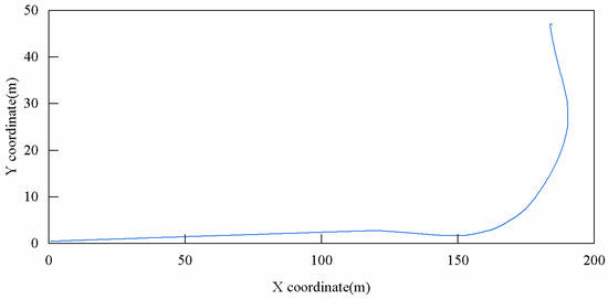
Figure 8.
Simulation Experiment 1 Trajectory.
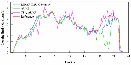
Figure 9.
Longitudinal velocity curve obtained by different methods in simulation experiment 1.
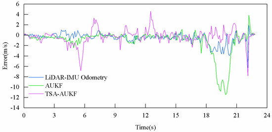
Figure 10.
Error curve in simulation experiment 1.
The driving trajectory in simulation experiment 2 is shown in Figure 11, and the vehicle velocity varies between 0–30 m/s. Figure 12 shows the longitudinal velocity of the vehicle obtained by different methods, and the error with respect to the longitudinal velocity reference value in Carla is shown in Figure 13. It can be clearly seen that TSA-AUKF still has better accuracy. A tunnel was passed between 28–37 s, resulting in a decrease in the performance of the LiDAR-IMU odometry. Predictions based on time-series analysis can be used to correct longitudinal velocity estimates. However, due to the lag of time-series analysis, there was a certain deviation in TSA-AUKF between 31–37 s.
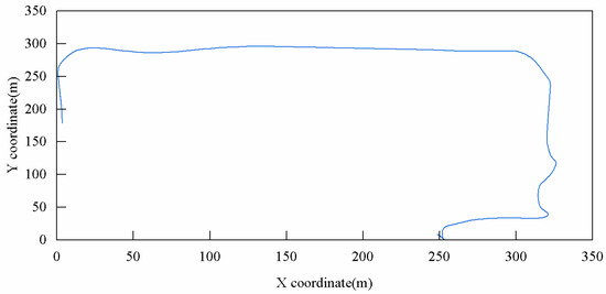
Figure 11.
Simulation Experiment 2 Trajectory.
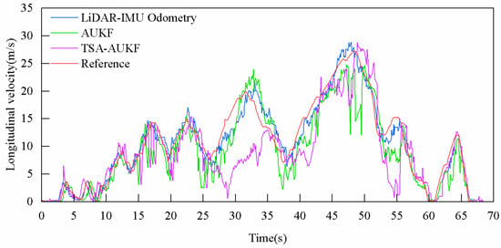
Figure 12.
Longitudinal velocity curve obtained by different methods in simulation experiment 2.
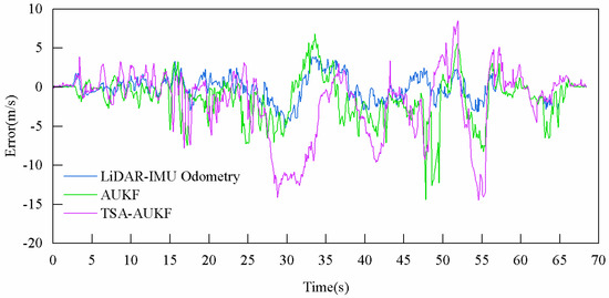
Figure 13.
Error curve in simulation experiment 2.
The root mean square errors (RMSEs) of LiDAR-IMU odometry, AUKF, and TSA-AUKF estimation results are shown in Table 2. In simulation experiment 1, compared with laser odometer and AUKF, TSA-AUKF can achieve approximately 37% and 55% performance improvements; in simulation experiment 2, compared with LiDAR-IMU odometry and AUKF, TSA-AUKF can achieve approximately 62% and 51% performance improvements.
Table 2.
RMSE of estimation error.
4.2. Real-Vehicle Experiment
Figure 14 shows the experimental platform. The platform’s sensors provide longitudinal reference velocity information of 10 Hz, LiDAR provides point cloud information of 10 Hz, IMU provides acceleration and angular velocity information of 100 Hz, and GPS provides positioning information of 5 Hz. Lidar, IMU, and GPS are installed in the red box position in Figure 14. Velodyne VLP-16 is used as a LiDAR sensor. The specifications of IMU are shown in Table 3.
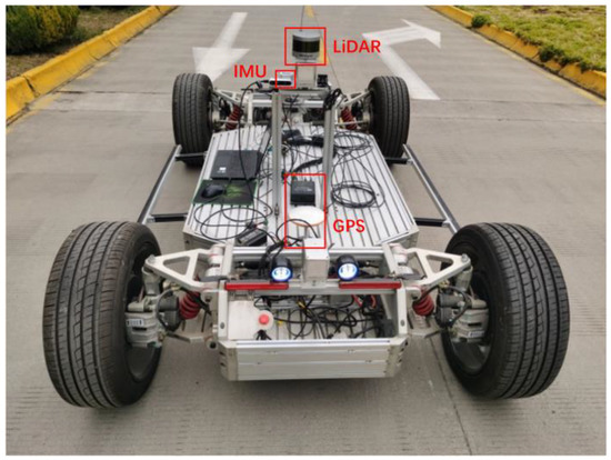
Figure 14.
Experimental platform.
Table 3.
Datasheet of LPMS-IG1.
The driving trajectory is shown in Figure 15, and the vehicle’s velocity varies between 0–5 m/s. In this experiment, we compared TSA-AUKA with the traditional GPS-IMU method. Figure 16 shows the longitudinal velocity of vehicles obtained using different methods, and the error with respect to the reference longitudinal velocity is shown in Figure 17. It can be clearly seen that TSA-AUKA can provide stable longitudinal velocity estimates.
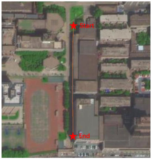
Figure 15.
Real-vehicle experimental trajectory.
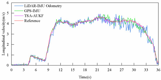
Figure 16.
Longitudinal velocity curve obtained by different methods in real-vehicle experiment.

Figure 17.
Error curve in real-vehicle experiment.
The RMSEs of LiDAR-IMU odometry, GPS-IMU, and TSA-AUKF estimation results are shown in Table 4. Compared with LiDAR-IMU and GPS-IMU, TSA-AUKF can achieve approximately 59% and 28% performance improvements.
Table 4.
RMSE of estimation error.
5. Conclusions and Future Work
This paper proposes a longitudinal velocity estimation method for driverless vehicles. By integrating LiDAR and IMU information, the goal of not relying on tires to represent longitudinal velocity is achieved, and the problem of GPS losing signal in certain areas can also be avoided. By using an adaptive noise estimator to track the statistical characteristics of system noise, model errors are reduced and filtering divergence is suppressed, thereby improving the robustness and filtering accuracy of the algorithm; introducing time-series analysis into the motion equation improves the estimation accuracy. The feasibility of the estimation method under medium- to high-velocity conditions was verified in simulation experiments. Under a velocity variation of 0–15 m/s, the RMSE of TSA-AUKF is 1.149 m/s; at a velocity variation of 0–30 m/s, the RMSE of TSA-AUKF is 1.573 m/s. In addition, the data drift generated by the simulation software can also verify the high robustness of the proposed algorithm. In real-vehicle experiments, TSA-AUKF achieved a 28% performance improvement compared to existing GPS-IMU longitudinal velocity estimation methods. The results show that the method proposed in this paper can provide stable longitudinal velocity estimates for driverless vehicles. In future work, more realistic vehicles will be used for experiments on standard roads to improve the performance of the algorithm.
Author Contributions
Conceptualization, C.Z. and Z.G.; investigation, Z.G.; methodology, C.Z. and Z.G.; project administration, M.D.; resources, M.D.; software, Z.G.; supervision, M.D.; validation, C.Z.; writing—original draft, Z.G.; writing—review and editing, Z.G. All authors have read and agreed to the published version of the manuscript.
Funding
This research was funded by the National Natural Science Foundation of China: Research on the Integrated Control Method of the Lateral Stability of Distributed Drive Mining Electric Vehicles (51974229), Shaanxi Innovative Talents Promotion Plan—Science and Technology Innovation Team (2021TD-27).
Institutional Review Board Statement
Not applicable.
Informed Consent Statement
Not applicable.
Data Availability Statement
Not applicable.
Conflicts of Interest
The authors declare no conflict of interest.
References
- He, H.W.; Peng, J.K.; Xiong, R.; Fan, H. An acceleration slip regulation strategy for four-wheel drive electric vehicles based on sliding mode control. Energies 2014, 7, 3748–3763. [Google Scholar] [CrossRef]
- Zhao, B.; Xu, N.; Chen, H.; Guo, K.; Huang, Y. Stability control of electric vehicles with in-wheel motors by considering tire slip energy. Mech. Syst. Sig. Process. 2019, 118, 340–359. [Google Scholar] [CrossRef]
- Arnold, E.; Al-Jarrah, O.; Dianati, M.; Fallah, S.; Oxtoby, D.; Mouzakitis, A. A survey on 3D object detection methods for autonomous driving applications. IEEE Trans. Intell. Transp. Syst. 2019, 20, 3782–3795. [Google Scholar] [CrossRef]
- Chen, W.; Tan, D.; Zhao, L. Vehicle sideslip angle and road friction estimation using online gradient descent algorithm. IEEE Trans. Veh. Technol. 2018, 67, 11475–11485. [Google Scholar] [CrossRef]
- Napolitano Dell’Annunziata, G.; Arricale, V.M.; Farroni, F.; Genovese, A.; Pasquino, N.; Tranquillo, G. Estimation of Vehicle Longitudinal Velocity with Artificial Neural Network. Sensors 2022, 22, 9516. [Google Scholar] [CrossRef] [PubMed]
- Karlsson, R.; Hendeby, G. Speed Estimation From Vibrations Using a Deep Learning CNN Approach. IEEE Sens. Lett. 2021, 5, 1–4. [Google Scholar] [CrossRef]
- Zhang, D.; Song, Q.; Wang, G.; Liu, C. A Novel Longitudinal Speed Estimator for Four-Wheel Slip in Snowy Conditions. Appl. Sci. 2021, 11, 2809. [Google Scholar] [CrossRef]
- Xin, X.S.; Chen, J.X.; Zou, J.X. Vehicle state estimation using cubature Kalman filter. In Proceedings of the 2014 IEEE the 17th International Conference on Computational Science and Engineering, Chengdu, China, 19–21 December 2014; pp. 44–48. [Google Scholar]
- Antonov, S.; Fehn, A.; Kugi, A. Unscented Kalman filter for vehicle state estimation. Veh. Syst. Dyn. 2011, 49, 1497–1520. [Google Scholar] [CrossRef]
- Li, J.; Zhang, J.X. Vehicle sideslip angle estimation based on hybrid Kalman filter. Math. Probl. Eng. 2016, 3269142, 1–10. [Google Scholar] [CrossRef]
- Xiong, L.; Xia, X.; Lu, Y.; Liu, W.; Gao, L.; Song, S.; Han, Y.; Yu, Z. IMU-Based Automated Vehicle Slip Angle and Attitude Estimation Aided by Vehicle Dynamics. Sensors 2019, 19, 1930. [Google Scholar] [CrossRef]
- Wang, Y.; Li, Y.; Zhao, Z. State Parameter Estimation of Intelligent Vehicles Based on an Adaptive Unscented Kalman Filter. Electronics 2023, 12, 1500. [Google Scholar] [CrossRef]
- van Zanten, A.T. Bosch ESP system: 5 years of experience. SAE Trans. 2000, 109, 428–436. [Google Scholar]
- Du, H.P.; Li, W.H. Kinematics-based parameter-varying observer design for sideslip angle estimation. In Proceedings of the 2014 International Conference on Mechatronics and Control, Jinzhou, China, 3–5 July 2014; pp. 2042–2047. [Google Scholar]
- Madhusudhanan, A.K.; Corno, M.; Holweg, E. Vehicle sideslip estimation using tyre force measurements. In Proceedings of the 2015 the 23rd Mediterranean Conference on Control and Automation, Torremolinos, Spain, 16–19 June 2015; pp. 88–93. [Google Scholar]
- Rezaeian, A.; Khajepour, A.; Melek, W.; Chen, S.K.; Moshchuk, N. Simultaneous Vehicle Real-Time Longitudinal and Lateral Velocity Estimation. IEEE Trans. Veh. Technol. 2017, 66, 1950–1962. [Google Scholar] [CrossRef]
- Pi, D.W.; Chen, N.; Wang, J.X.; Zhang, B.J. Design and evaluation of sideslip angle observer for vehicle stability control. Int. J. Automot. Technol. 2011, 12, 391–399. [Google Scholar] [CrossRef]
- Li, X.; Chan, C.Y.; Wang, Y. A reliable fusion methodology for simultaneous estimation of vehicle sideslip and yaw angles. IEEE Trans. Veh. Technol. 2016, 65, 4440–4458. [Google Scholar] [CrossRef]
- Farrell, J.A.; Tan, H.S.; Yang, Y. Carrier phase gps-aided ins-based vehicle lateral control. J. Dyn. Syst. Meas. Control 2003, 125, 339–353. [Google Scholar] [CrossRef]
- Yoon, J.H.; Peng, H. A cost-effective sideslip estimation method using velocity measurements from two gps receivers. IEEE Trans. Veh. Technol. 2014, 63, 2589–2599. [Google Scholar] [CrossRef]
- Song, R.; Fang, Y. Vehicle state estimation for INS/GPS aided by sensors fusion and SCKF-based algorithm. Mech. Syst. Signal Process. 2021, 107315, 0888–3270. [Google Scholar] [CrossRef]
- Gao, L.; Ma, F.; Jin, C. A Model-Based Method for Estimating the Attitude of Underground Articulated Vehicles. Sensors 2019, 19, 5245. [Google Scholar] [CrossRef]
- Talebi, S.P.; Godsill, S.J.; Mandic, D.P. Filtering Structures for α-Stable Systems. IEEE Control Syst. Lett. 2023, 7, 553–558. [Google Scholar] [CrossRef]
- Lv, J.; He, H.; Liu, W.; Chen, Y.; Sun, F. Vehicle Velocity Estimation Fusion with Kinematic Integral and Empirical Correction on Multi-Timescales. Energies 2019, 12, 1242. [Google Scholar] [CrossRef]
- Wang, X.; You, Z.; Zhao, K. Inertial/celestial-based fuzzy adaptive unscented Kalman filter with Covariance Intersection algorithm for satellite attitude determination. Aerosp. Sci. Technol. 2016, 48, 214–222. [Google Scholar] [CrossRef]


Disclaimer/Publisher’s Note: The statements, opinions and data contained in all publications are solely those of the individual author(s) and contributor(s) and not of MDPI and/or the editor(s). MDPI and/or the editor(s) disclaim responsibility for any injury to people or property resulting from any ideas, methods, instructions or products referred to in the content. |
© 2023 by the authors. Licensee MDPI, Basel, Switzerland. This article is an open access article distributed under the terms and conditions of the Creative Commons Attribution (CC BY) license (https://creativecommons.org/licenses/by/4.0/).