Supervised Learning Technique for First Order Multipaths Identification of V2V Scenario

Abstract

In geometrical localization techniques, the propagated signal’s first-order multipath (FOMP) characteristics are used to calculate the location based on geometrical relationships. Utilizing the characteristics of higher order multipath (HOMP) results in a significant localization error. Therefore, distinguishing between FOMPs and HOMPs is an important task. The previous works used traditional methods based on a deterministic threshold to accomplish this task. Unfortunately, these methods are complicated and insufficiently accurate. This paper proposes an efficient method based on supervised learning to distinguish more accurately between the propagated FOMP and HOMP of millimeter-Wave Vehicle-to-Vehicle communication in an urban scenario. Ray tracing technique based on Shoot and Bounce Ray (SBR) is used to generate the dataset’s features including received power, propagation time, the azimuth angle of arrival (AAOA), and elevation angle of arrival (EAOA). A statistical analysis based on the probability distribution function (PDF) is presented first to study the selected features’ impact on the classification process. Then, six supervised classifiers, namely Decision Tree, Naive Bayes, Support Vector Machine, K-Nearest Neighbors, Random Forest, and artificial neural network, are trained and tested, and their performance is compared in terms of HOMP misclassification. The effect of the considered features on the classifiers’ performance is further investigated. Our results showed that all the proposed classifiers provided an acceptable classification performance. The proposed ANN showed the best performance, whereas the NB was the worst. In fact, the HOMP misclassification error varied between 2.3% and 16.7%. The EAOA exhibited the most significant influence on classification performance, while the AAOA was the least.

1. Introduction

The most effective localization methods in a challenging environment, such as urban environments, are vehicle-to-vehicle (V2V) and vehicle-to-infrastructure (V2I) [1]. In such techniques, the localization process can be established using either a communication technique based on sharing information or a transmission technique based on utilizing the multipath components (MPCs) [2,3]. However, the communication technique still faces latency and reliability challenges, especially in urban environments, although the 5G and millimeter-Wave (mm-wave) communication technologies have been widely used to meet the massive data transmission demand [4]. The transmission techniques (also called geometric-based) are proposed to handle this challenge in several research. The localization concept of the geometric-based techniques involves exploiting the characteristics of FOMP, such as path length, angle of arrival, and angle of departure, to localize the vehicle based on geometrical relationships [5,6,7]. For example, in [7], the propagation time and angular characteristics of the FOMPs are utilized to allow a sensing vehicle (SV) to localize the hidden vehicle (HV). Unfortunately, in multipath environments (i.e., urban areas), the propagation phenomenon of the signal between two blocked transceivers is a combination of FOMPs and HOMPs [8,9,10,11]. 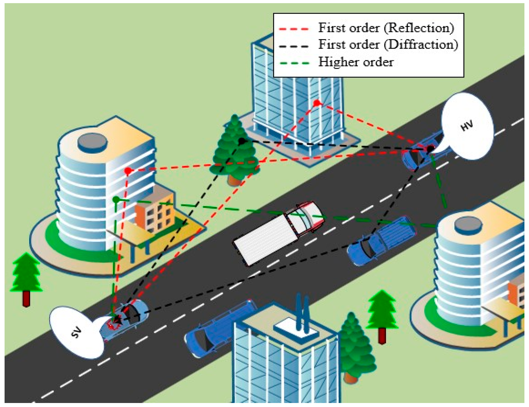Figure 1 shows the types of propagation paths that can be established between HV and SV. However, mistakenly using HOMP’s characteristics rather than FOMP’s characteristics is considered a major challenge in geometric-based techniques. It has a negative impact on localization accuracy. Therefore, detecting the FOMPs among the HOMPs is important for achieving precise localization.

So far, various techniques have been proposed for distinguishing between the FOMPs and HOMPs. These techniques, in brief, are mainly relied on a statistical condition of the characteristics of the received signal. For instance, the authors in [12] assumed a determined level of the received signal as a threshold to identify the FOMP. In the same manner, the time of arrival (TOA) based on a proximity detection method is utilized in [11]. The authors in [13,14] presented an analytical model to characterize the path loss as a threshold to identify the FOMPs. Unfortunately, methods that rely on a deterministic threshold exhibit complexity, owing to the necessity of the complex analyses, and the inaccuracy particularly in high-frequency bands (mm-wave bands), due to the challenge of identifying the exact threshold. The inherent sparsity of the mm-wave channel causes disordering of the propagation path characteristics of the transmitted signal. This leads to the absence of a precise threshold and in turn introduces misjudgment in the distinguishing process. Therefore, to break through the drawbacks of this method, a classification technique based on machine learning (ML) is proposed to distinguish the FOMPs.

In ML tools, such as supervised learning classification models, the classification decision is created based on a previous training process. Such methods have a good classification performance provided that the features of the training data are carefully prepared. In general, the classification performance of ML models is affected by two main factors: the features of the training dataset, and the hyperparameters of the model. More details about the classifiers will be presented in Section 3.1. However, in wireless communications aspects, the MPCs, such as received power, propagation time, and angle of arrival and departure, have been utilized as features of the training data for various purposes in the literature. Generally, these characteristics can be extracted either from experiments, based on measurement, or from simulation tools [15,16]. The experimental methods have difficulties and high costs especially when a large amount of data is required. Therefore, the researchers resort to simulation tools instead of experimental methods.

Typically, the simulation tools that have been utilized for this purpose, are built on either empirical (stochastic) or deterministic models. The empirical models rely on observation and measurement based on theoretical analysis to predict propagation characteristics. Meanwhile, the deterministic models leverage geometric optics. Ray tracing is one of the deterministic modeling methods. It provides high accuracy and more reliable predictions for the propagation path characteristics of high-frequency communication networks, i.e., mm-wave bands. Therefore, it has been considered to predict the propagation characteristics of 5G networks and beyond in several research [17,18,19]. Since this work is basically concerned about mm-wave bands; thus, the ray tracing technique will be considered a predation model of the propagation characteristics. Readers can refer to the reference [16] for more details about the channel modeling techniques.

However, the major contributions of this work are as follows:

• We presented a statistical analysis of the characteristics of the propagation paths and investigated how these characteristics impact the FOMPs identification.
• We proposed an efficient solution based on supervised classifiers to distinguish between the FOMP and the HOMP in blocked V2V communication by applying six supervised classifiers. The training dataset was generated by using a ray tracing technique.
• We tested the proposed classifiers using different strategies. Then their performance is compared in terms of several well-known metrics such as accuracy and precision. Furthermore, since this work is interested in the FOMPs, we presented a particular metric based on the estimation error of the HOMP as FOMP.

The rest of this paper is organized as follows, after this protracted introduction, a review of the related works is presented in Section 2. Then, a brief explanation of ML is provided in Section 3. The methodology of this research is described in Section 4. In Section 5, an analysis of the obtained results is presented including validation of the ray tracing predictions, statistically analyzing the propagation characteristics, and discussing the performance of the proposed classifiers. Finally, the conclusion is drawn in Section 6.

2. Related Works

Typically, in the localization aspect, the classification methods have been used either for identifying the FOMPs or for identifying the Line of Sight (LOS) and Non-Line of Sight (NLOS). Therefore, the related works in this paper are presented in two parts. The first part highlights the works that utilized the conventional techniques based on the deterministic threshold for FOMPs identification, while the second part highlights ML for LOS and NLOS identification. The proposals that used conventional techniques to identify LOS and NLOS are ignored.

Earlier, the FOMPs and HOMPs identification methods have been presented in [11] based on proximity detection technique. They used TOA to normalize the weighting factor of the path; thus, the HOMPs are identified as outliers. In a similar vein, an iterative strategy based on the generalized likelihood ratio test is proposed in [20] to detect the FOMPs and HOMPs of the downlink. In these methods, a complex analysis is required. However, since the power of the transmitted signal is strongly attenuated by the reflection; therefore, the received power had been utilized to distinguish between the FOMPs and HOMPs in several works, [8,21,22] are among them. However, the obtained results in [2] illustrated that, the received power alone could not be used to accurately distinguish between the FOMPs and HOMPs. However, in summary, the traditional methods are complex and insufficiently accurate.

However, motivated by the efficient performance of ML classifiers, it has been widely used to solve classification problems in the literature for several aspects. In the localization field, the supervised classification models became popular for LOS and NLOS identification. The researchers utilized different direct or indirect characteristics of the paths as an input vector. For instance, the authors in [23] discriminated LOS paths and NLOS according to the Rician k factor. In [24], the authors combined the angular information of the mm-wave channel with the features, such as RMS delay spread, kurtosis, and Rician K factor, to train the SVM in order to identify the LOS and NLOS. They showed that the features in the angular domain significantly improved the accuracy of the SVM model. The non-temporal configurations (frequency characteristics) of the channel impulse response of Ultra-wideband signal are exploited as an input vector for training the Convolutional Neural Network (CNN) model to extract the features, the CNN output is then used to feed the Long Short Term Memory Network (LSTM) model [25]. High accuracy of LOS/NLOS classification has been achieved in that work, but there are also highlighted limitations such as the authors didn’t investigate the influence of the obtained classification on the position estimation; furthermore, the diffraction effects were limited in the training data. The angular parameters of the mm-wave channel have been utilized in [26] to identify LOS and NLOS environments. The author proposed a neural network model named angle information learning neural network. The angular parameters have been used to learn the proposed model. That work achieved identification accuracy of up to 99.41%.

Based on the above review, we have observed that, the deterministic threshold is adopted for identifying the FOMPs. Meanwhile, ML is still not used for this purpose. ML has been widely used for identifying the LOS and NLOS. We also observed that the traditional methods are complicated and not accurate enough. This has motivated us to propose an identification method by employing ML to distinguish between the FOMPs and HOMPs. The features of the training dataset are considered based on some of the characteristics that have been used to identify the LOS and NLOS. In particular, five well-known classifiers namely Decision Tree (DT), Naive Bayes (NB), Support Vector Machine (SVM), K-Nearest Neighbors (KNN), and Random Forest (RF), are considered. Furthermore, an artificial neural network (ANN) model is proposed, as it has become very popular nowadays.

3. Background on ML Classifiers

Basically, this work aims to apply supervised ML techniques for distinguishing the FOMPs and HOMPs. Therefore, this section is dedicated to presenting a brief explanation of the supervised classifiers, the features of the training dataset, and performance evaluation criteria.

3.1. Supervised Classisfication Algorithms

Supervised classifiers are one of the most popular techniques in data mining aspect. Its working principle is creating a decision based on analysis of the data that have been entered previously. Typically, the classification process of the supervised classifiers consists of two phases. The first phase is learning based on the training. In this phase the labeled data is used to train the model to generate the prediction algorithm. The second phase is classification, where the trained model is used to predict the label classes. However, there are several supervised classification models have been proposed for different purposes in the literature. In this part, a brief discussion about the five most popular classifiers, is presented. Additionally, a brief discussion of the ANN learning model, which is widely utilized in the same context of our study. However, more information about the supervised classifiers can be found in the reference [27].

DT classification algorithm is the most well-known. The fundamental principle of its classification algorithm is by utilizing a top-down technique through the tree to search for a proper decision. The tree is built based on the training data. The decision is established based on a series of sequence processes. The DT algorithm can be used with both linear and nonlinear numerical data. It has fast learning and is easy to understand and interpret. On the other hand, overfitting data is more likely to occur. The algorithm of the NB classifier basically relies on Bayes’ formula. In NB, the features are grouped independently, and the features are assumed not related to each other. Similar to DT, the NB classification has fast learning. In addition, there is not a too large amount of data required for training.

SVM can be used for regression and classification problems. It is most popular for binary classification. SVM’s algorithm consists of two stages. First, the data is mapped into n-dimensions. Then, the hyperplane is used to classify the data into two classes. However, the SVM’s performance is affected by the noisy data. The KNN algorithm is also considered one of the simplest classifiers. The classification decision of the KNN algorithm is taken based on the number of neighborhoods, i.e., the value of K. Therefore, different values of K may obtain a different classification. The value of K is usually set to an odd number. It is also determined by the trial-and-error method. This is considered the main disadvantage of the KNN algorithm. Nonetheless, on the other hand, the KNN algorithm is more robust even with noisy data. RF algorithm is basically a combination of multiple DT. The trees are randomly created. Therefore, it is called a random forest. It is presented to overcome the DT overfitting problem, where the decision is made based on the subset of the training data in parallel and the final output is generated by combining the output of the individual trees.

In terms of the training time, usually, the RF model requires a higher compared to the DT model, but the prediction results of RF models outperform the DT models in most cases. However, NN and deep learning algorithms have become popular in the last few years. It has been widely used to solve linear and non-linear problems whether it is classification or regression. Its learning concept is adjusting the weights of the neurons to reduce the error of the prediction. Several models of NN have been presented in the literature, such as ANN (single layer), DNN (multiple layers: input layer, hidden layers, output layer), CNN, and LSTM. However, the prediction accuracy of these models is higher and more robust, i.e., is not affected by the noisy data. On the other hand, compared to the previous models, these models have deprived interpretation.

3.2. Features Selection

Consider the V2V scenario as shown in Figure 1. The established transmission system between the vehicles is used for localization, where the sensing vehicle desires to localize the hidden vehicle by utilizing the characteristics of the transmitted signal. According to [28] the characteristics of the transmission channel of the multipath components (MPCs) at the receiver (sensing vehicle) can be expressed as follows

$$H\left(t\right)=\sum _{n=1}^N{{\rho }_{n}e}^{-j\mathrm{\varnothing }k}\delta \left({\gamma }_n\right)\delta \left({\mathrm{\varnothing }}_n\right)\delta \left({\theta }_n\right)$$

(1)

where, N is the number of received MPCs. ${\rho }_n$ and ${\gamma }_n$ are respectively the complex amplitude and the delay of the Nth received path. ${\theta }_n$ and ${\mathrm{\varnothing }}_n$ are the angle of departure and arrival of the received path, respectively. They also represent the horizontal and vertical angles of each path. However, from Equation (1), we can directly obtain several characteristics of the MPC, such as the received power, delay, and horizontal and vertical angles. In the following, a brief explanation of the impact of these characteristics for distinguishing the type of propagation path.

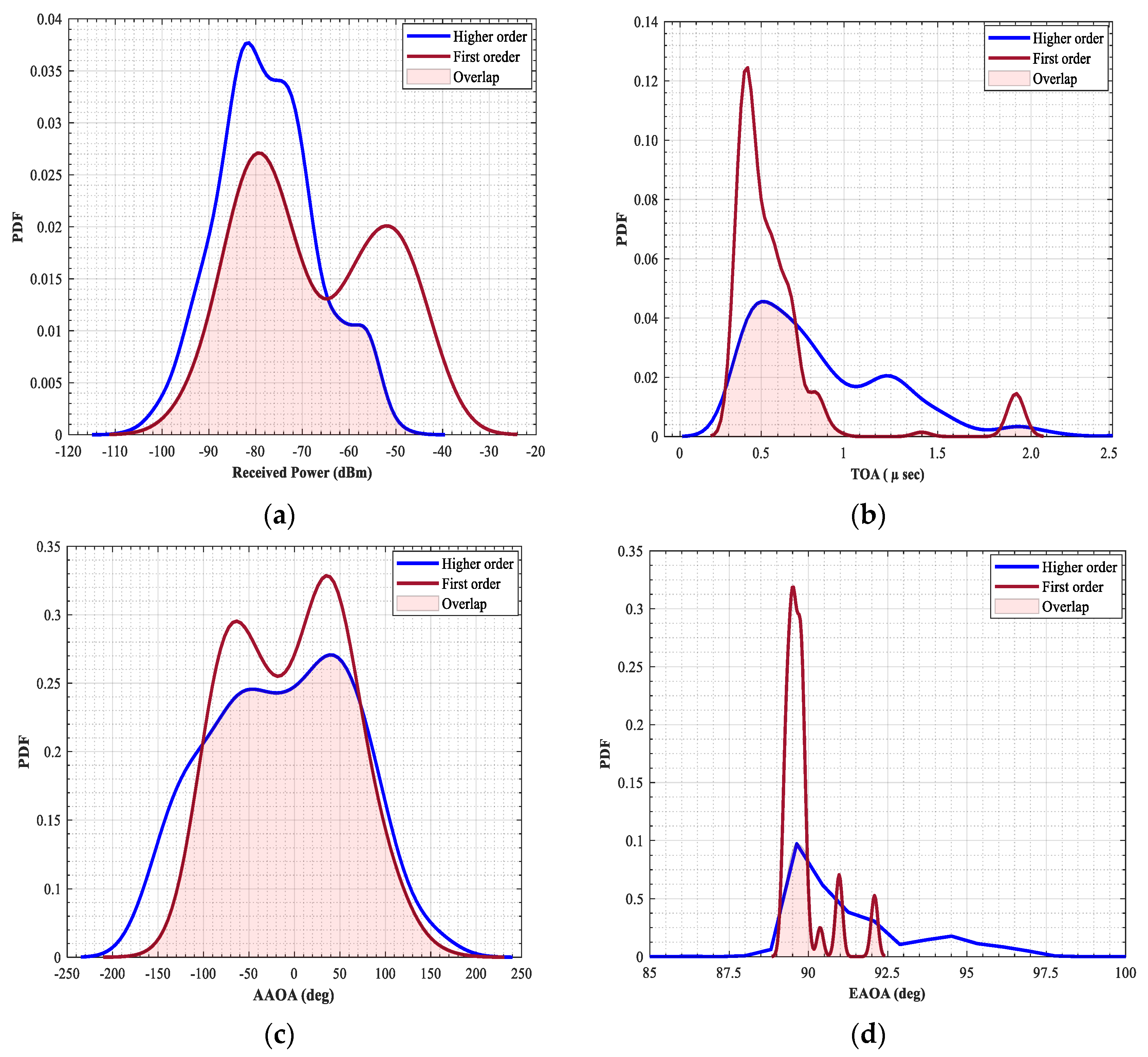
3.2.1. Received Power (RP)

Logically, the FOMPs include the amount of received power more than the HOMPs. Often the FOMPs are the dominant paths that carry a significant amount of power. The more reflections the more power losses. Therefore, the received power can be considered as a feature to distinguish the type of paths. However, some of the propagated paths are scattered by the edge of the buildings. These paths usually contain a lower amount of received power even though they are FOMP. Thus, ambiguity will occur if the identification relies on the received power stand-alone.

3.2.2. Propagation Time

It is defined as the measurement of the required time for the transmitted signal to reach the receiver through a relative propagation path. Generally, the propagation time of the HOMPs is larger than the FOMPs. The presence of more reflections in the path propagation leads to a higher propagation delay at the time of arrival (TOA). This feature can be integrated with the previous feature to improve the accuracy of classification.

3.2.3. Angular Variation

The direction of the incoming signal is also called the angle of arrival (AOA). It can be accurately estimated in mm-wave systems thanks to multiple input multiple output antenna (MIMO). Therefore, it has been exploited for positioning purposes [29]. However, AOA can be measured horizontally or vertically; they are called azimuth and elevation respectively. Basically, the azimuth angle of arrival (AAOA) is related to the layout of the surrounding environment, while the elevation angle of arrival (EAOA) is related to the propagation path length, especially when the transmitter and receiver have different heights.

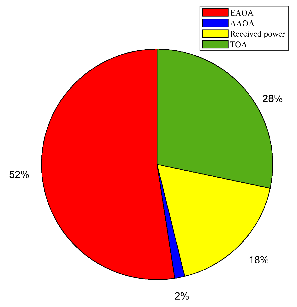
In summary, the considered input vector of the training data can be expressed as follows X = {Received power, delay, AAOA, EAOA} of the nth arrived path of each snapshot.

3.3. Assessment Criteria

In order to evaluate the performance of ML classifiers, the prediction results of the model should be assessed. There are several well-known metrics have been presented in this regard. The most popular metrics are accuracy, precision, receiver operating characteristic (ROC), mean absolute error (MAE), and root mean squared error (RMSE).

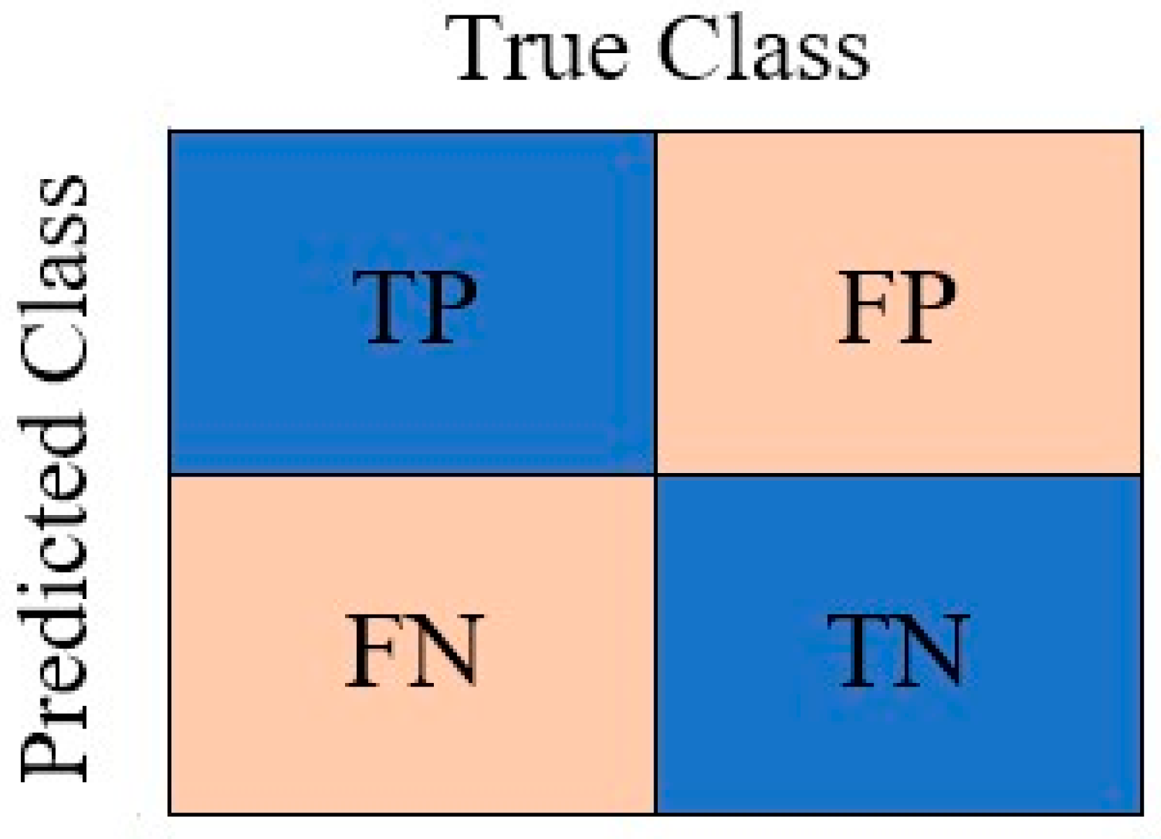
Assume a confusion matrix of the binary classification model, as shown in Figure 2, where the positive is considered to represent FOMP, while the negative is considered to represent HOMP. The true positive (TP) denotes the FOMPs that are truly predicted as FOMPs. The false positive (FP) denotes the HOMPs that are predicted as FOMPs. The false negative (FN) denotes the FOMPs that are predicted as HOMPs. The true negative (TN) denotes the HOMPs that are truly predicted as HOMPs.

3.3.1. Accuracy

It is the ratio of all samples that are accurately predicted to all samples. It can be calculated as

$$\mathrm{A}\mathrm{c}\mathrm{c}\mathrm{u}\mathrm{r}\mathrm{a}\mathrm{c}\mathrm{y}=\frac{TP+TN}{TP+FP+FN+TN}$$

(2)

3.3.2. Precision

It is the ratio of the TP samples to all samples that are predicted as positive samples (i.e., TP and FP). Its formula is

$$Precision=\frac{TP}{TP+FP}$$

(3)

3.3.3. Recall

It is the ratio of TP samples to the total correct predicted samples (TP and FN). It can be calculated by

$$ROC=\frac{TP}{TP+FN}$$

(4)

3.3.4. Mean Absolute Error (MAE)

It is the absolute error between the actual classes and the predicted classes. It is expressed by

$$MAE=\frac{\sum _{i=1}^n|X_i-Y_i|}{n}$$

(5)

where $X_i$ and $Y_i$ are the actual and predicted class respectively.

3.3.5. Root Mean Squared Error (RMSE)

It is also used to represent the difference between the actual classes and the predicted classes. It is expressed by

$$RMSE=\sqrt{\frac{\sum _{i=1}^n{(X_i-Y_i)}^2}{n}}$$

(6)

The above metrics are standard, they have been widely used for evaluating the performance of the classifiers in various aspects. In this work, we are interested in the HOMP misclassification (the actual HOMP that have been predicted by the classifier as a FOMP) which will produce more localization errors. Therefore, the most important metrics in our work regard are accuracy and precision because their formula consists of the FP. Meanwhile, the recall metric is not important in our case, since the FOMPs that are predicted by the classifier as HOMPs will be ignored, i.e., the localization accuracy won’t be affected. However, MAE and RMSE metrics represent the classification errors including the FOMP and HOMP. However, we also define additional metric for performance evaluation as follows:

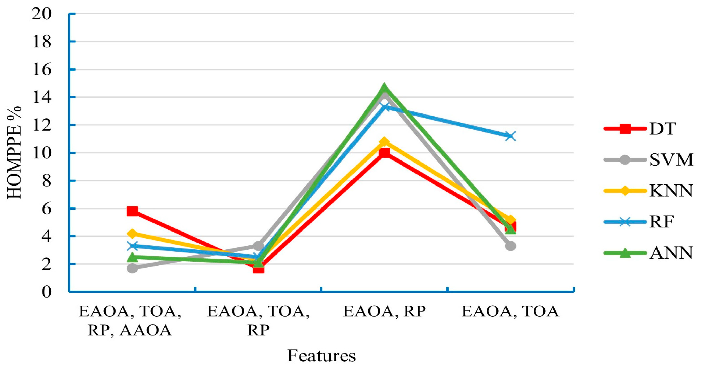
3.3.6. HOMP Prediction Error (HOMPPE)

It is the ratio of the misclassification HOMPs (FP) to the total actual HOMPs.

$$HOPPE=\frac{FP}{FP+TN}$$

(7)

4. Methodology

The main purpose of this work is to present an efficient method to distinguish between the FOMPs and HOMPs based on supervised classification. The ray tracing technique will be used to generate the dataset. Therefore, the methodology of this work is divided into three parts. The first part explains the simulation setup. The second part illustrates the configuration of V2V communication scenario and how the dataset is collected. The third part describes the method of applying the supervised classifiers to achieve the purpose of this work.

4.1. Simulation Setup and SBR Validation

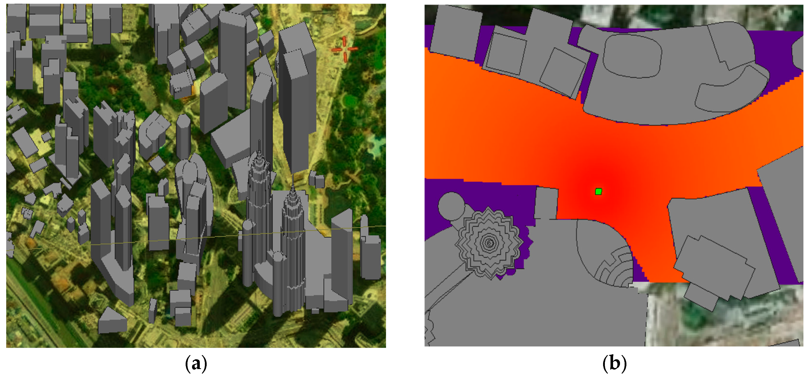
Wireless InSite (WI) software, developed by Remcom, is used to model the realistic V2V scenario in the considered urban environment, which is Kuala Lumpur City Centre (KLCC), Jalan Ampang. To create a geometric structure (buildings detailed) of the interested area, a real 3D model of KLCC is downloaded first from the Cadmapper website [30]. Then, this 3D model is prepared and converted into dxf format by using SketchUp application. Finally, the dxf file is imported to WI simulation as shown in Figure 3a. The values of electromagnetic (EM) parameters of buildings, leaves, and objects were set based on [31,32]. The EM parameters of the simulation setup are listed in

Table 1. Parameters of the simulation setup.

EM of Material Properties
Electro Magnetic Parameters	Material	ɛr	σ [S/m]
	Buildings (Concrete)	5.31	0.8967
	Vegetation-Leaf	26	0.39
	Vegetation-Branch	20	0.39
	Vehicle (Metal)	1.00	10 × 107
UMi specifications
Antenna	Type	Omnidirectional
	Polarization	Vertical
	Gain	27 dBi
	Height	Transmitter = 10 m Receiver = 2 m
Transmitted Power		42.0 dBm
UMi size		200 m × 400 m
Frequency		28 GHz
Ray tracing Technique		SBR
Model		Full 3D

.

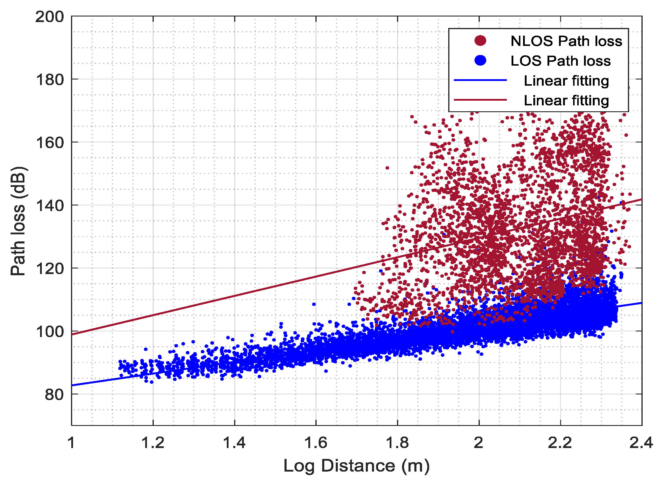
In order to verify the validity of the ray tracing results, an urban 5G micro cell (UMi) scenario is formed with dimensions of 200 m × 400 m in the considered environment as shown in Figure 3b. The parameters of the formed UMi are listed in Table 1. The specifications of the formed UMi are inspired by [33,34]. The performance of the UMi is analyzed and compared with the previous works in terms of received power (often modeled by path loss) for LOS and NLOS conditions. It is worth mentioning that, the prediction correctness of the ray tracing simulator is validated based on the received power only, where it is more relevant to the buildings’ layout and materials (i.e., user-defined). Regarding the predictions of the other propagation characteristics, such as propagation time and angular properties, it is mainly defined by the designer of the ray tracer simulator. Therefore, they are not going to be involved in the validation.

4.2. V2V Configuration and Data Collection

In this part of the methodology, first, we explain the established V2V scenario. Then, present the data processing including the method of obtaining the paths’ characteristics from the ray tracing simulation and labeling the obtained data.

The established V2V scenario is inspired by Figure 1. The vehicles are blocked from each other, there are no existing direct paths between the vehicles. Three boxes (objects) have been created to present the HV, SV, and blockage (the vehicle in between). The dimensions of the HV and SV objects are 4.5 m (length), 2 m (width) and 1.5 m (height). Meanwhile, the blockage dimensions are set to 5 m (length), 4 m (width), and 4 m (height). The transmitter and receiver antennas are located on the top of the HV and SV with a height of 2 m. The model is considered to be single input single output (SISO) for simplicity purposes. The types of both antennas are selected to be isotropic antennas with vertical polarization. The transmission power is set to 14.6 dBm. The separated distance between the vehicles is varied in range from 20 m to 50 m as the normal distance between two blocked vehicles in the real world. In order to simplify the simulation, the vehicles are assumed to be stationary (no mobility) while capturing the path characteristics. Note that, the typical speed of the vehicle in urban environments is less than 50 Km/h. Therefore, with the high sampling rate, the change of nominal characteristics will be very small, i.e., the assumption is reasonable. We select mm-wave at 28 GHz frequency band with a channel bandwidth of 450 MHz, which is a candidate in Release 15 of 5G for outdoor wireless communications, as the operating frequency. Ray tracing technique based on SBR is utilized to predict the propagation path characteristics. The maximum number of propagation paths is set to 25, where a large number of propagation paths will not improve the prediction accuracy of the propagation characteristics in the simulation results [35]. The parameters of the V2V configuration are depicted in

Table 2. V2V configuration parameters.

Antenna	Type	Isotropic
	Polarization	Vertical
	Gain	10 dBi
	Height	Transmitter = 2 m Receiver = 2 m
Transmitted Power		14.6 dBm
Frequency		28 GHz
Bandwidth		450 MHz
Number of reflections		6
Number of Paths		25
Ray Spacing		0.15
Ray tracing Technique		SBR
Model		Full 3D

.

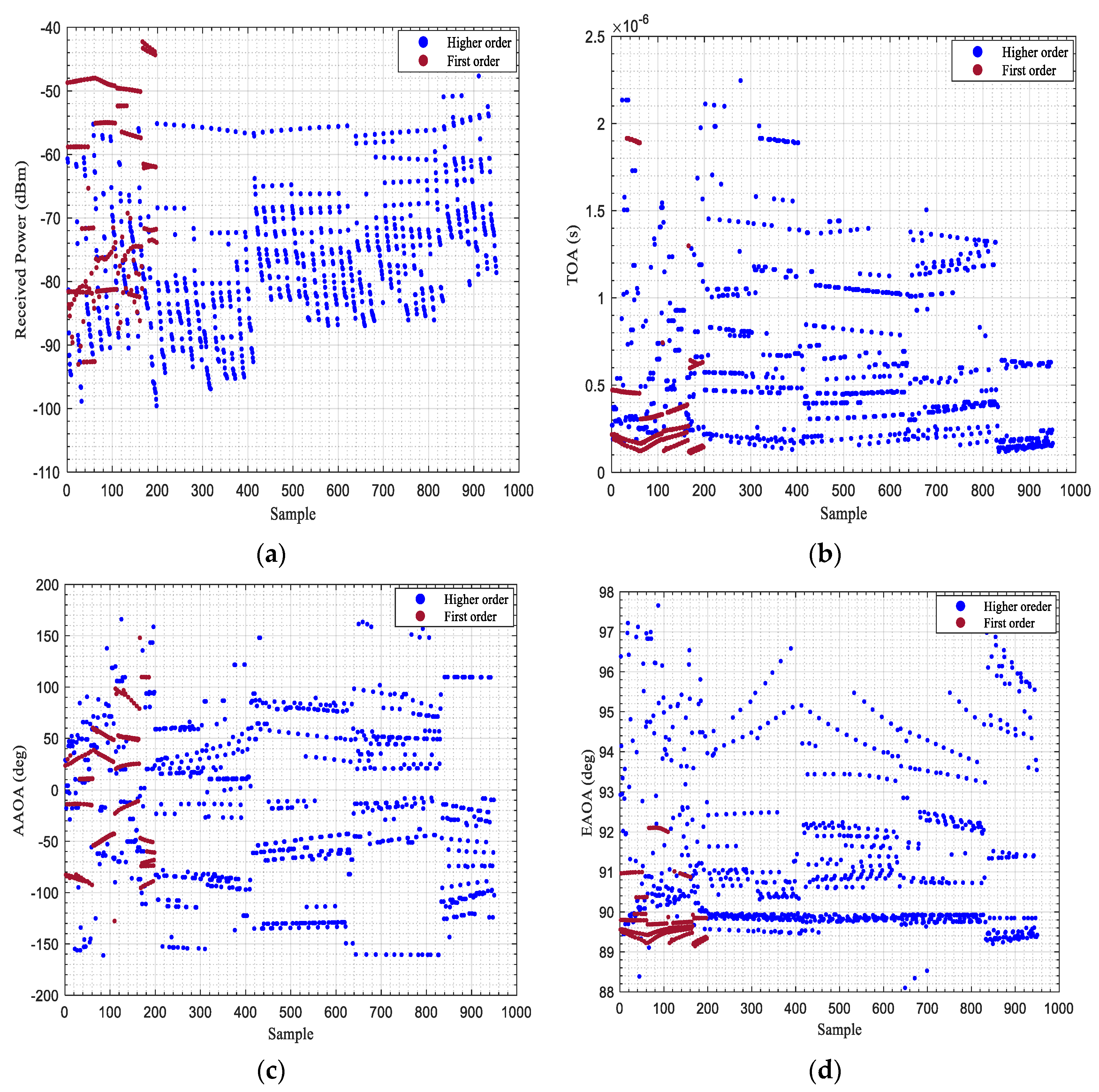
In terms of dataset collection, the SBR technique is utilized for predicting the characteristics, i.e., received power, propagation time, and horizontal and vertical angle of arrival, of each propagated path that arrived at the receiver (SV). A total of various 46 locations are selected to record the data in order to include the effect of reflections on a variation of parameters of the received signal. The data are recorded for 25 paths at each location. This means that 1150 samples are collected while the simulation is running.

4.3. Data Preparation and Supervised Classification Models

This section elaborates on the process of preparing the dataset for training the classifier including labeling the data and dividing it into training, validating, and testing. In addition, this section also discusses the setup and configuration of the proposed classifiers. However, WI enables us to visualize the propagation mechanism of the paths. Based on this visualization, the stored data are manually labeled into binary classes (i.e., 0 and 1). Where the FOMPs are labeled as 0′s class, and the HOMPs are labeled as 1′s class. After labeling the data, a shuffling method is used for dividing the data for training, validation, and testing the classifiers. 85% of the data are used for training and validating the proposed classifier respectively, whereas 15% of the data is used for testing the proposed classifiers. Since the training data is imbalanced, (the number of HOMPs (1′ class) is around three times more than the number of FOMPs (0′s class)), in addition, the data size is not too large, a random over-sampling method is applied to handle this issue. Furthermore, the k-fold cross-validation technique is used to protect classifier performance against overfitting. In the k-fold cross-validation technique, the dataset is randomly divided into 10 partitions (folds) for training and validation, where each folder includes the same values of labels. Then, the classifier is trained using the training data, and its performance is assessed by using validation data. Finally, the average of validation errors over all files is calculated. This means that the classifier will be trained and validated with all the data.

In binary classifiers, the mathematical model is formulated using a decision function that maps the input vector X = [RP, TOA, EAOA, AAOA] to a binary output label Y = (0 or 1). The decision function is presented based on the classification algorithm. The objective of training the classifiers is to minimize the average value of the binary cross-entropy loss function. The classifier predicts the class as an optimization problem based on the learning method by adjusting the weights (w) and biases (b). The binary cross-entropy loss can be defined as:

$$\min ‖-[Ylog\widehat{Y}+(1-Y)log(1-\widehat{Y})]‖$$

(8)

$$\widehat{Y}=w^{t}X+b$$

(9)

where, $w$ denotes the vector weights assigned to each feature, b represents the terms that modify the decision boundary of the classifier. In terms of the configuration and setup of the classifiers, the MATLAB classification learner app is used to design, train, validate, and test the proposed classifiers. For the training process, the Bayesian optimization algorithm is utilized. However, in order to prevent the overfitting of the classification learner, we enabled the validation method as mentioned before. Furthermore, since the obtained data is not highly dimensional, there are only four features used for classification; thus, the principal component analysis (PCA) won’t be activated in the classification learner. The training parameters, such as learning rate, earlier stop the training, etc., were set based on the default. Regarding tuning the hyperparameters of the classifiers, each classifier has specific hyperparameters. For example, the type of kernel for SVM, number of trees for RF, value of k for KNN, number of hidden layers, layer size (number of neurons), and activation function for the ANN. Trail and test method is used to select the optimal hyperparameter of the proposed classifiers.

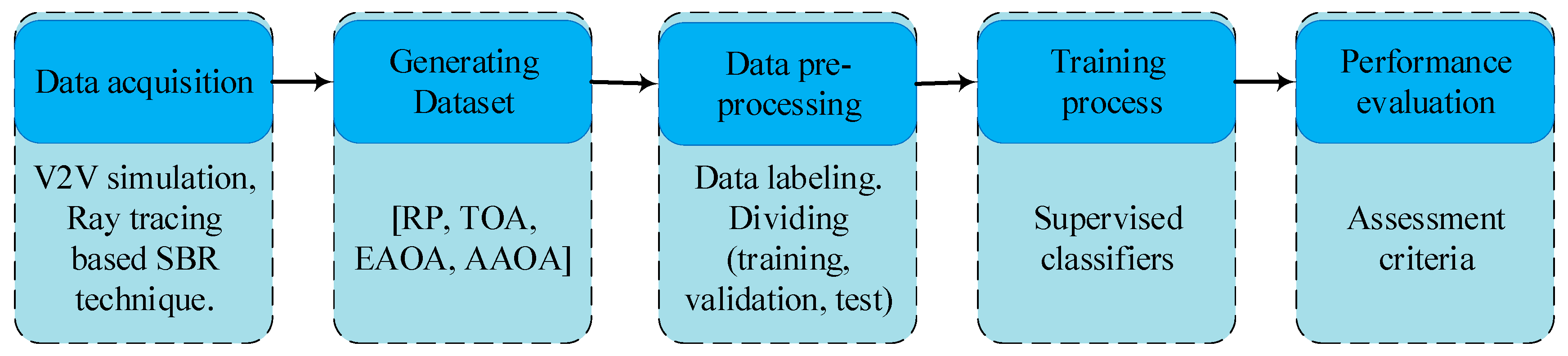
However, for comparative purposes, all the proposed classifiers are trained using the same training dataset. Then, the classifiers are validated by using the same validation data. Finally, the performance of each classifier is evaluated based on the same test data. The workflow of the proposed supervised classification method is shown in Figure 4.

5. Result and Discussion

This section is dedicated to providing analysis of the obtained result from the simulation. However, since the training dataset is obtained based on the predictions of the SBR technique; therefore, the reliability of this technique will be verified in Section 5.1. After that, we will present a statistical analysis of the obtained data, i.e., the characteristics of the propagation paths in Section 5.2. Finally, the prediction results of the proposed classifiers will be discussed in Section 5.3.

5.1. Ray Tracing Validation

In order to verify the validity of the ray tracing results, we compare the performance of each of the formed UMi and the real UMi in terms of path loss parameters. The formed UMi, in Figure 3b, consisted of a total of 12,015 receivers. 8251 receivers (69%) are located in LOS (red area) with BS (green square), whereas 3764 receivers (31%) are located in NLOS (blue area). The recorded values of the path loss from the simulation at each receiver are shown in Figure 5. It is clear that, the recorded path loss values of NLOS receivers are higher than LOS path loss values; Moreover, the path loss is increased as the distance to the base station is increased. However, based on the linear regression technique, the equation of the Close-In model is used to fit and calculate the parameters of path loss, i.e., the path loss exponent and the standard deviation. The results show that the path loss exponent values for LOS and NLOS were 2.148 and 3.095 respectively, meanwhile, the standard deviations for LOS and NLOS were 6.404 dB and 9.39 dB respectively. However, the literature reported that, in UMi, the calculated values of path loss exponent using Close-In based-linear regression at 28 GHz takes different values for LOS and NLOS scenarios. Normally it ranges from 2 dBm to 4 dBm for LOS (2 for free space and 4 for lossy environments) and 2.7 dBm to 6 dBm for NLOS high reflections [36,37,38,39]. It is obvious that, the values of path loss exponent for LOS and NLOS are involved in these ranges. Therefore, the predictions correctness of the utilized SBR technique is verified. The comparison of the path loss parameters of the simulation and the previous works is depicted in

Table 3. Path loss parameters for simulation and previous works.

Scenario	Parameters	Outdoor Urban Environment
		Previous Work [36,37,38,39]	Simulation
LOS	n	2–4	2.148
NLOS	n	2.7–6	3.095

.

5.2. Statistical Analysis of the Propagation Characteristics

This section presents an analysis of the obtained characteristics. The purpose of this analysis is to study the contributions of the characteristics in distinguishing between the FOMPs and HOMPs. However, the obtained results of the considered characteristics, i.e., received power, TOA, AAOA, and EAOA, of 1150 MPs recorded at 46 different locations are shown in Figure 6. However, 200 of them were FOMPs (red dots), while 950 were HOMPs (blue dots). It is clear that from the obtained results, the number of the FOMPs is lower than the HOMPs, which is consistent with the literature, where the HOMPs are dominant propagation in a multipath-reach environment. As shown in Figure 6, the distributions of the captured samples of all paths, whether FOMPs or HOMP, fluctuated and dispersed. The AAOA showed the highest degree of dispersal for FOMPs and HOMPs, whereas the EAOA showed the lowest. The TOA and received power of the captured samples showed a critical degree of scattering. For example, the recoded received power for FOMPs and HOMPs ranged from −42 dBm to −92 dBm and −46 dBm to −100 dBm respectively. In general, all the captured samples of the characteristics showed that there is no existence of a threshold that separates the samples of the FOMPs from HOMPs perfectly. This means that the inaccuracy of distinguishing between FOMPs and HOMPs based on a deterministic threshold is therefore investigated.

In order to better understand the contributions of these characteristics in distinguishing the FOMPs and HOMPs, a statistical analysis is presented based on the probability distribution functions (PDF) as shown in Figure 7. The PDF graphs demonstrate that all extracted characteristics showed different degrees of the overlapped area between the FOMPs and HOMPs. Also, we can observe that, the PDF graphs of the FOMPs are generally centralized to a certain value; meanwhile, in HOMPs, they have a relatively flatted. However, the ratio of the overlapped area to the total area of the PDF of FOMPs and HOMPs is shown in Figure 8. It is clear that the overlap ratio of the EAOA is the lowest; on the other hand, the AAOA was the highest. The overlap ratio of the received power (RP) and TOA are 47.92 and 35.38 respectively. From this analysis, we concluded that the EAOA might provide the highest contribution to the distinction between FOMPs and HOMPs. The TOA comes in the second order. Meanwhile, the AAOA might provide the lowest contribution. We also concluded that, it is quite hard to identify whether they are FOMPs or HOMPs based on a single characteristic. Therefore, the characteristics of the propagated path should be jointly utilized in order to improve the performance of the classifiers.

5.3. Discussion of Classification Results

As mentioned before, the classification learner application in MATLAB has been used to implement the six proposed classifiers. However, this section presents a discussion and comparison of the prediction performance of the proposed classifiers, as well as addresses the impact of features on the prediction performance.

5.3.1. Evaluation of the Classifiers Prediction

In order to evaluate the performance of the proposed classifiers, their prediction results are evaluated and compared in terms of the presented metrics in Section 3.3 (i.e., accuracy, precision, recall, MAE, RMSE, and HOMPPE). However, it is impossible to present a comparison between the proposed classifier directly, since each classifier has specific hyperparameters. Therefore, the optimal hyperparameters of each classifier are selected first. Then the comparison is conducted.

Table 4. Hyperparameters configuration of the proposed classifiers.

Classifier	Optimized Hyperparameters
DT	Max. No. of split: 50
NB	-
SVM	Kernel function: Gaussian.
KNN	K: 7, Distance metric: Euclidean.
RF	Max. No. of split: 30, Number of destination trees: 15.
ANN	No. of layers: 3, Layers size: 40, Activation function: ReLU, Max. No. of epochs: 500.

shows the optimal selection of the most important hyperparameters of the proposed classifiers. These parameters are selected based on an empirical method. The tradeoff between the HOMPs misclassification ratio, accuracy, time of training, and testing has been considered during the selection of the optimal hyperparameters.

However, the comparison of the prediction results of the optimized classifiers is shown in

Table 5. Comparison of the prediction results of the proposed classifiers.

Classifier	Accuracy %	Precision %	HOMPPE %	MAE	RMSE
DT	94.5	92.9	5.8	0.061	0.247
NB	87.8	91.8	16.7	0.135	0.368
SVM	92.4	85.7	2.7	0.041	0.203
KNN	94.1	96.4	4.2	0.047	0.217
RF	95.9	92.9	3.3	0.041	0.203
ANN	96.5	92.9	2.3	0.034	0.184

. As mentioned earlier, the most important metrics in the evaluation of the classifier’s performance are accuracy, precision, and HOMPPE. Thus, in order to evaluate and compare the performance of the classifiers, these metrics must be taken into account jointly. Obviously, from the results in the table, all the proposed classifiers have provided a good classification performance except the NB. The ANN classifier achieved the best performance. Where the HOMPPE, the accuracy, and the precision of the ANN classifier were 2.3%, 96.5%, and 92.9% respectively. However, since the HOMPPE is considered the most important metric in the evaluation; thus, the SVM classifier comes in the second order (although its accuracy and precision are lower than the DT, KNN, and RF), it achieved 2.7%, 95.9%, and 0.83% for HOMPPE, accuracy and precision respectively.

However, the NB classifier was the worst among the six classifiers. Basically, the NB algorithm assumes that the features are unrelated and independent, but the features of our training data are related to each other. For example, the FOMPs are usually assigned by higher received power, lower propagation time, and higher EAOA as shown in the analysis in the previous subsection. Therefore, the NB algorithm achieved the worst classification performance with this type of data compared to the other classifiers. Although the DT and the RF algorithms have the same principle of classification, the RF outperformed the DT. The interpretation of that, the RF utilizes the power of multiple DT. It does not depend on the feature importance given by an individual DT.

Based on the obtained results, it is obvious that the presented methods have provided an efficient and accurate classification with lower complexity compared to the traditional methods. There was no more analysis required. The disadvantage of the presented method lay in the cost of generating the dataset in the real world.

5.3.2. Impact of the Features Selection

The presented statistical analysis of the selected characteristics (training features), in Section 5.2, revealed a different overlapped area for each of them. Based on this analysis, we discuss the impact of these features on the classifiers’ performance. In particular, we shall use various features to train the classifiers and then evaluate their performance. The proposed NB classifier is excepted from the comparison. The evaluation and comparison are conducted in terms of the accuracy and the HOMPs misclassification.

Figure 9 depicts the scores of the importance of the ranking of the features obtained from the MATALB classification learner. It is obvious that the scores of importance are in the same consistency with the presented PDF analysis in Section 5.2. The EAOA showed the highest scores of importance; meanwhile, the lowest score of importance is shown in the AAOA. In other words, statistical analysis can be utilized to select more affectable features to achieve a higher level of classification performance rather than the empirical method.

The comparison of the impact of feature selection on the accuracy and HOMPPE are shown in Figure 10 and Figure 11 respectively. It’s clear that, for all the proposed classifiers, the accuracy is slightly increased and the HOMPs error is slightly decreased when the AAOA feature is unselected. It means that the AAOA confused the classifiers since there was too much overlap between the AAOA of the FOMPs and HOMPs. However, due to the high impact of the TOA on the classifiers, the performance of the classifiers is degraded (the accuracy dropped and the HOMPPE increased) when the TOA feature is removed from the training dataset and only the EAOA and received power (RP) are selected. However, as mentioned before, the TOA and the received power have a quite similar scores of importance. Therefore, the performance of the classifiers (i.e., the accuracy and the HOMPPE) is slightly different when the TOA or received power are alternatively selected jointly with the EAOA as features of the training data.

6. Conclusions

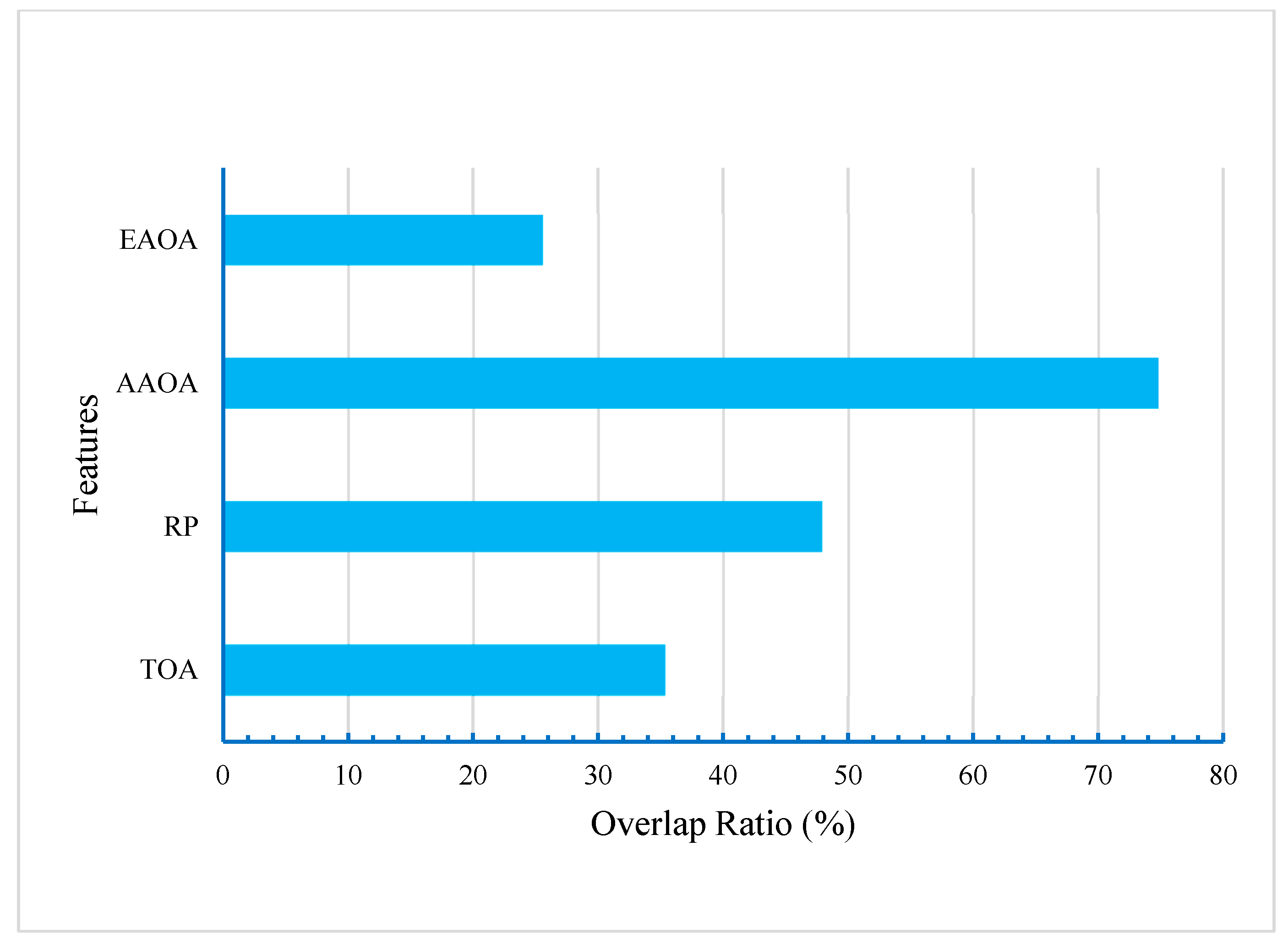
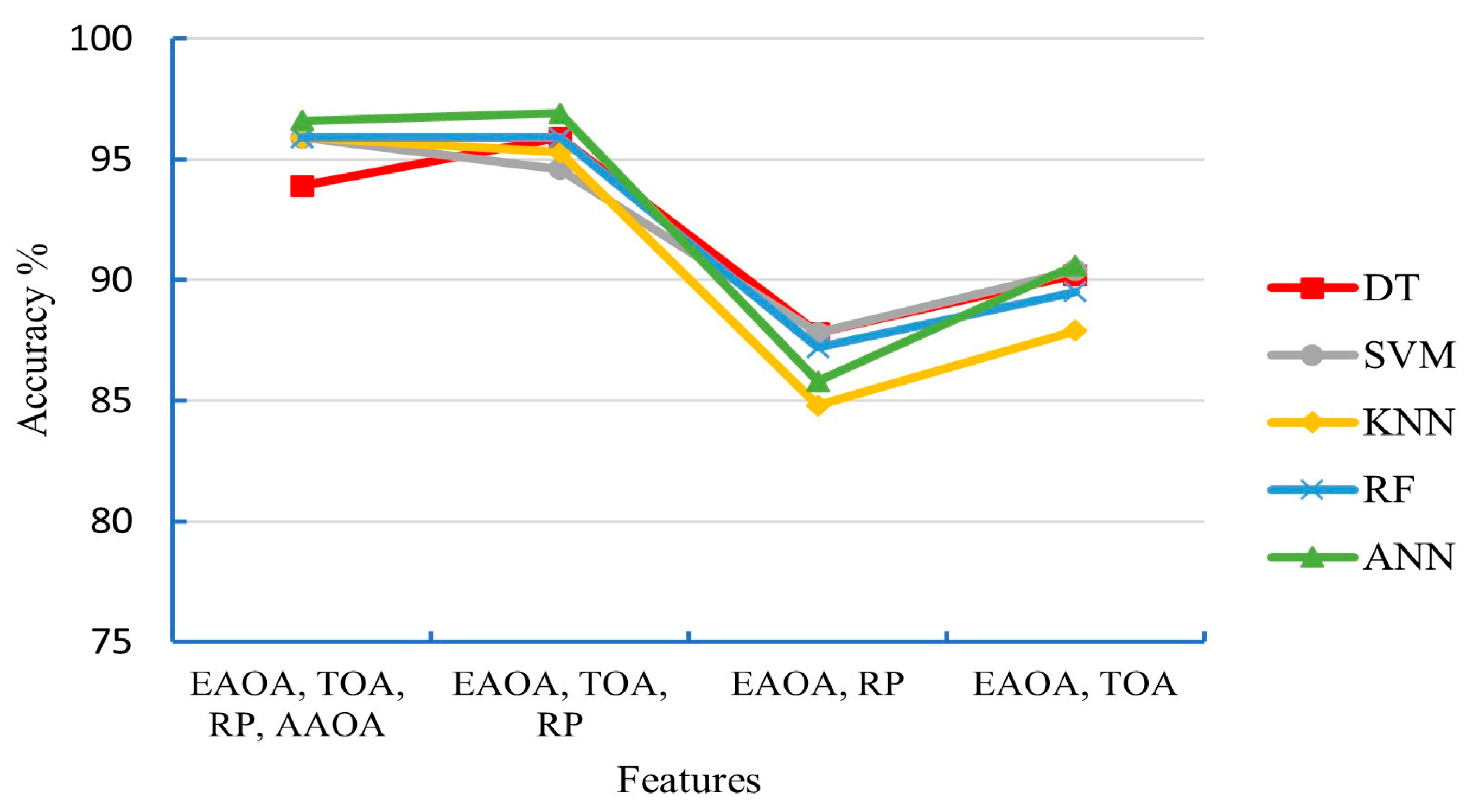
V2V localization technique based-geometric has been presented in various research breaking through the drawbacks of the GPS technology in urban environments. This technique relies mainly on utilizing the characteristics of the FOMPs. Mistakenly utilizing the HOMPs instead of the FOMPs is considered the most challenging issue in this technique. However, this work proposed a supervised ML classifiers to accurately distinguish between the FOMPs and HOMPs. The characteristics of the path propagation, that have been obtained from the predictions of the ray tracing based on the SBR technique, have been considered as input features of the training dataset. In this work, a statistical analysis of the obtained characteristics is presented first. Then, six supervised classifiers, namely DT, NB, SVM, KNN, RF, and ANN have been proposed and tested and their performance has been compared in terms of accuracy, precision, and HOMPPE. The comparison results showed that the accuracy of the proposed classifiers ranged from 87.8% to 96.5%. This means that the characteristics of the path propagation are efficient features for training the classifiers. The ANN classifier achieved the best performance, while the SVM classifier came in the second order. Whereas the NB achieved the worst performance. In terms of HOMPPE (HOMPs misclassification), it was 2.3% in the best classifier (i.e., ANN) and 16.7% in the worst classifier performance (i.e., NB). The impact of the training features selection on the performance of the proposed classifiers has been further investigated in this work. We concluded that the results of the statistical analysis are strongly consistent with the contribution of the training feature. In conclusion, distinguishing between FOMP and HOMP based on the proposed method using the characteristics of the propagation signal is more efficient and has a lower complexity compared to the traditional methods.

However, in this work, the considered features of the training dataset were directly extracted from the simulation. To improve the performance of the classifiers, we recommend involving more features for future work, such as the power delay profile of the received signal and the layout details of the surrounding area.