Abstract
In this paper, we address the problem of trajectory tracking control of autonomous vehicles by considering the nonlinear characteristics of tires. By considering the influence of the tires’ dynamics on steering stability, the proposed predictive controller can track the desired trajectory and desired velocity in the presence of road curvature while minimizing the lateral tracking deviation. First of all, a hierarchical control structure is adopted, in which the upper-level controller is used to calculate the desired acceleration and the desired front-wheel angle to maintain the control target, and the lower-level controller realized the command through the corresponding component devices. Moreover, a force estimator is designed based on the radial basis function (RBF) neural network to estimate the lateral force of the tires, which is incorporated into the boundary conditions of the vehicle envelope constraint to improve the adaptability of the controller to the vehicle performance. Finally, the proposed controller is tested by co-simulation of CarSim (a simulation software specifically for vehicle dynamics)/Simulink (a modular diagram environment for multidomain simulation as well as model-based design) and hardware-in-loop simulation system. The co-simulation and experimental results demonstrate the controller safely driving at the vehicle’s handling limits and effectively reduce the slip phenomenon of the vehicle.
1. Introduction
Autonomous vehicles have a great potential in improving traffic flow and safety performance, which makes the technology of autonomous vehicle more and more popular, especially in developed countries and emerging markets [1,2]. As one of the important components of autonomous vehicles, the trajectory tracking control system aims to track the desired trajectory by controlling the actuators of the steering wheel, brake and throttle [3]. The high nonlinearity of the vehicle dynamics will make it difficult for the trajectory tracking controller to ensure the tracking accuracy and stability of the vehicle at the same time [4]. Therefore, a good trajectory tracking control system should fully consider the road information and the nonlinearities characteristics of tires.
In order to address the trajectory tracking problem, much research has been devoted to selecting the suitable control algorithms, such as the linear quadratic regulator (LQR) [5,6], fuzzy control [7,8], the sliding mode control (SMC) [9,10] and the proportional-integrated-differential (PID) control [11]. However, the constrains caused by tires during trajectory tracking cannot be fully considered in these controller design. In recent years, the model prediction control (MPC) methods have been widely used in trajectory tracking control, which is characterized by rolling optimization and dealing with the optimization problem while considering the input and output constraints [12]. A large number of researches indicate that the MPC algorithms are good at dealing with the trajectory tracking control problems with the multi-constraints [13,14]. Some researches converted the trajectory tracking control problem based on the MPC controller that considering vehicle stability and environmental constraints [15] or collision avoidance restraints [16]. Some researches improve trajectory tracking accuracy by adaptively adjusting the weight matrix in the target function [17,18]. In addition, a kinematic cascade MPC-PID controller with side slip angle compensation was designed in Ref. [19] to solve the trajectory tracking control problem of high-speed autonomous vehicles. The authors of [20] proposed a dead-band penalty function to solve the inequality constraints and guarantee smoothness of the solution.
More precise vehicle models can improve the controller’s ability to predict the future behavior of the vehicle. Banginwar proposed a real-time predictive vehicle controller by using Pontryagin’s optimization method in Ref. [21]. Meanwhile, Raigoza enhanced the trajectory tracking method with automatic collision avoidance in Ref. [22]. The authors of [23] designed a MPC controller, which takes the 8-degree-of-freedom vehicle model as the prediction model and the 14-degree-of-freedom vehicle model as the control object to achieve trajectory tracking. The Unscented Kalman Filter (UKF) was used in Ref. [24] to estimate the vehicle states, which were used to judge vehicle stability. Although the MPC method with a prediction function could significantly improve the trajectory tracking accuracy, it needed to repeatedly solve optimization problems at each control step, which leads to a heavy computing burden and potential risks in real-time control. In addition, some constraints have a great impact on the trajectory tracking performance of the vehicle, such as the slip and body deviation [25]. Therefore, a suitable equivalent model of vehicle dynamics should be constructed by considering the reasonable constraints
Ignoring the aerodynamics and gravity, the tire force plays a critical role in improving the vehicle’s handling performance. However, most researches limited the tire model to the linear area [26]. With increasing the vehicle speed, the nonlinearity caused by the tires’ dynamics had an influence on the trajectory tracking accuracy, even the handling stability. In Ref. [27], the piecewise linear approximation of the tire characteristic curve method and root mean square error (RMSE) were used to obtain segmented points in different regions to improve the approximate accuracy of the tire models. By combining regularization with continuous linearization, a nonlinear tire model was established to estimate the lateral force of the tire. In addition, Mammar et al. [28] derived the tire cornering stiffness and slip angle based on the tire characteristics to establish a tire model. However, the piecewise affine (PWA) tire model and tire cornering stiffness estimation are only the approximation of the tire model in a limited area, which could not capture the nonlinearity evident for the trajectory tracking control. Thus, the tires’ dynamics should be fully considered.
It is essential to guarantee the vehicle stability, and it should be mentioned that equilibrium analysis [29] or empirical judgment methods [30] are indeed needed to judge vehicle stability, along with the vehicle stability judged using the envelope constraints [31]. The lateral velocity as a boundary condition for the envelope constraints could not be obtained from the sensors directly. Considering that the lateral velocity can be estimated accurately as presented in Refs. [32,33], the lateral velocity could be gained as a configuration, which is set as the input of the envelope constraint of the vehicle swing.
Motivated by the above discussion, this paper presents a trajectory tracking controller design with consideration of the tires’ dynamics and slip constraints. The innovations of the paper are summarized as follows:
- Proposing a MPC controller by considering the tires’ dynamics and the road curvature for the trajectory tracking control;
- Designing a tire force estimator based on the radial basis function (RBF) neural network to estimate the vehicle driving states, which are used to update the slip constraint.
- Conducting the co-simulation (CarSim/Simulink) and Hardware-in-loop (HIL) platform to validate the performance of the proposed trajectory tracking control system.
The remainder of this paper is organized as follows. In Section 2, the control strategy of the trajectory tracking control system is described. In Section 3, a trajectory tracking model is established based on the trajectory tracking control system. In Section 4, based on the MPC algorithm, the trajectory tracking problem considering the slip constraint is solved. In Section 5.1, the CarSim/Simulink co-simulation platform is constructed to verify the effectiveness of the envelope constraint under extreme driving states and test that the vehicle can still drive effectively beyond the nonlinear region of the tire, and it is compared with the algorithm proposed in Ref. [34]. In Section 5.2, the HIL platform is built, and the effectiveness of the algorithm is verified based on the quintic polynomial function trajectory planning, and it is compared and verified with the co-simulation. Section 6 summarizes the contents of this paper.
2. Proposed Trajectory Tracking Control System
A hierarchical control structure is proposed to construct the controller for the trajectory tracking control system, as shown in Figure 1. The overall goal of the control strategy is to calculate the desired front-wheel steering angle and longitudinal acceleration and implement this control target via the corresponding component devices to eventually tracking the desired trajectory. The control structure consists of two sub-controllers, which are the upper-level controller and the lower-level controller. The functional implementation of the upper-level controller is divided into two parts, including the vehicle trajectory tracking model and control law, which are used to collect the state between the vehicle and the desired trajectory and driver input, and then compute the desired front-wheel steering angle and desired longitudinal acceleration. The lower-level controller realizes the output of the upper-level controller via the steering and driving devices to track the desired trajectory.
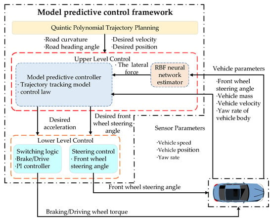
Figure 1.
Hierarchical control structure of the trajectory tracking control system.
3. Trajectory Tracking Model
A valuable vehicle model can improve the smoothness of the vehicle during driving and the handling stability of the vehicle during real-time control of autonomous vehicles. Thus, in this section, the trajectory tracking model is established by considering the force of the tires, as shown in Figure 2.
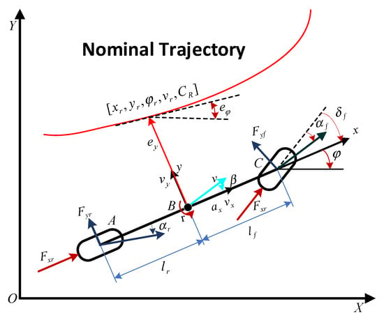
Figure 2.
Trajectory tracking model schematic.
The model is established based on the following assumptions:
- The influence of road slope is not taken into account;
- The coupling relationship between longitudinal and lateral forces is ignored; only the pure cornering characteristics of the tire is considered;
- The load transfer of the tire is ignored;
- The air resistance is ignored;
The heading error and longitudinal velocity error are defined as:
where represents the orientation error of the yaw angle with respect to the desired trajectory, and is the error between the current and the desired longitudinal velocity.
The desired yaw rate is obtained:
where is the road curvature.
Thus, combined Equation (1) with Equation (2):
The assumption for the heading error is small; can be defined as:
The vehicle dynamics model can be described by the following differential equations:
where is the generalized longitudinal acceleration of the vehicle; and are the distance from CG(center of gravity) to the front/real axle; is the longitudinal force of the front wheel; is the longitudinal force of the rear wheel; and is the front-wheel steering angle. The lateral force of the front/rear wheel and Fyr are functions of the slip angle of the tire, which can be calculated in the following ways:
where is the road friction coefficient, and represents the total vertical load of the vehicle.
The slip angles and indicate the angle between the wheel velocity and the direction of the wheel itself:
The total vertical load of the vehicle is distributed between the front and rear wheels according to the geometry of the car model, described by the parameters and :
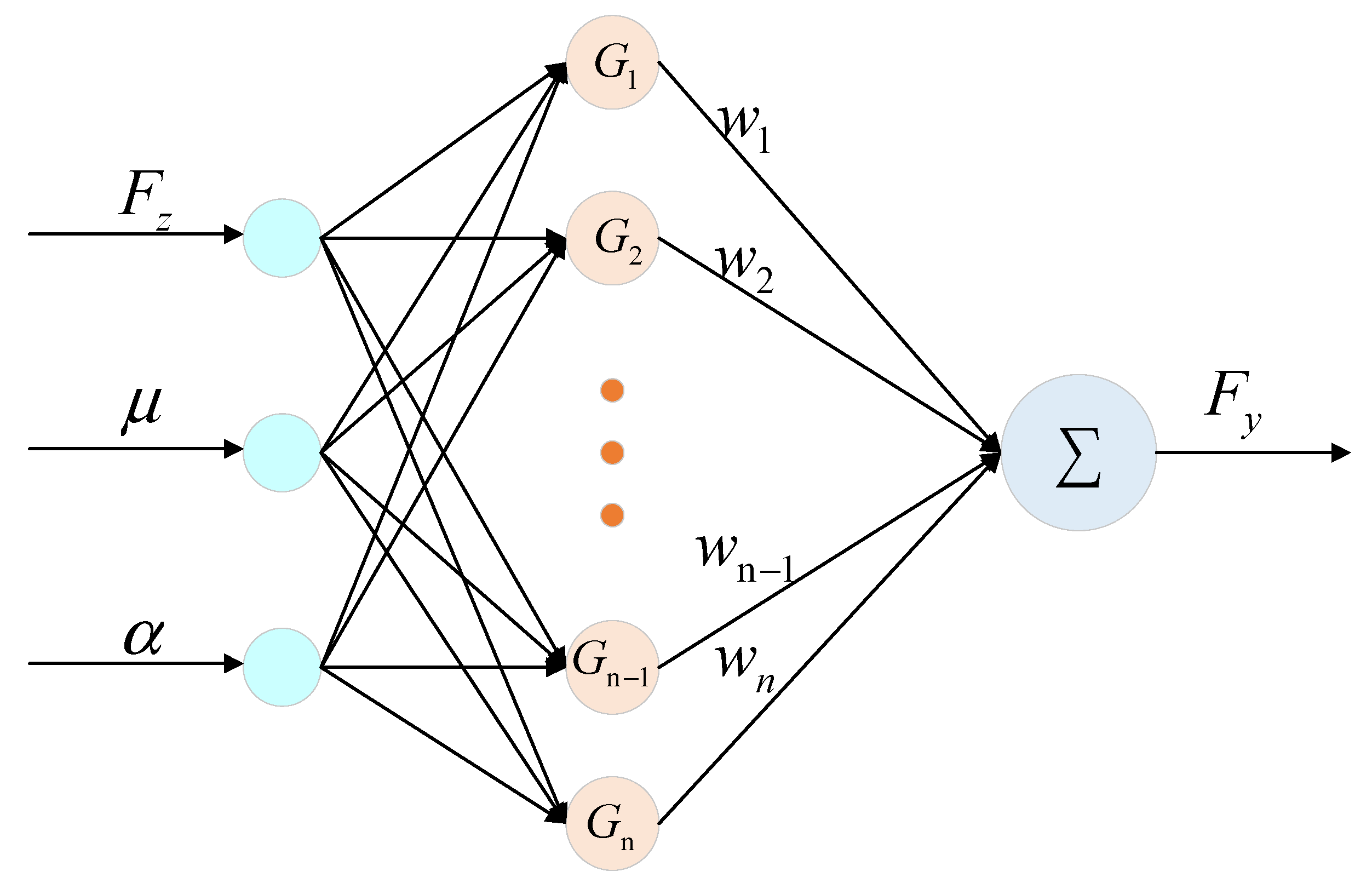
By analyzing Equation (6) and considering tire characteristics, we find that there are three main factors affecting the lateral force : the vertical load , the road friction coefficient , and the slip angle α, which is a complex nonlinear time-varying function with three inputs and one output. It is difficult to establish its accurate mathematical model with traditional methods, so this paper establishes a neural network model of the lateral force by the characteristics of the RBF neural network approximation of nonlinear functions as shown in Figure 3. The neural network consists of three layers. The first layer is the input layer, which consists of three input quantities: . The second layer is the hidden layer, and the activation function adopted by the hidden layer is a Gaussian function:
where is the center width of the hidden layer; X is the input vector; is the central unit of the jth radial basis function, which is the same as the input vector X dimensionality. The third layer is the output layer, which is the output lateral force , and its solution is:
where is the weight.
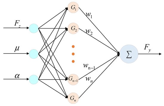
Figure 3.
RBF neural network model for the lateral force.
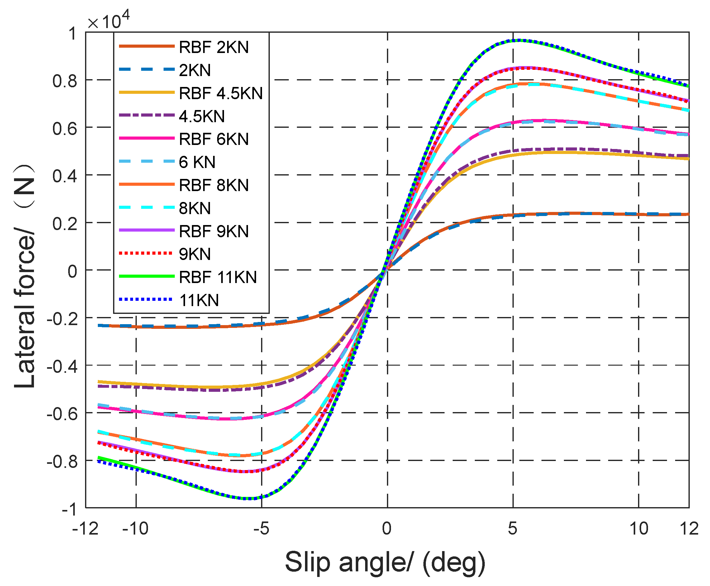
When the road friction coefficient is fixed, the lateral force is estimated by the RBF neural network as shown in the Figure 4:
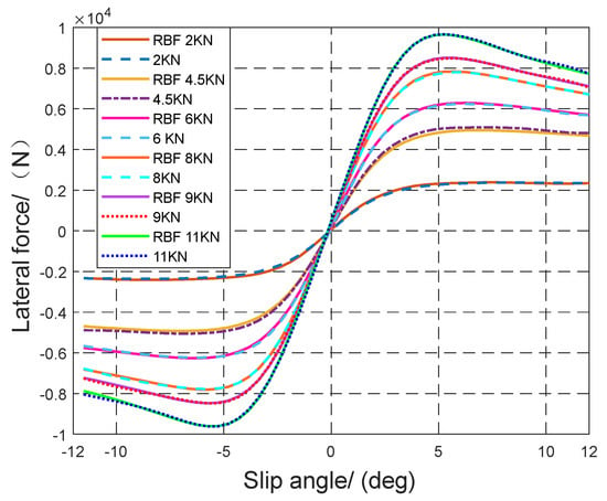
Figure 4.
The estimated lateral force of RBF neural networks under different vertical loads.
As shown in Figure 4, the lateral force estimator based on the RBF neural network can estimate the lateral force of the tire well.
Equations (3)–(10) can be combined to obtain the nonlinear vehicle dynamics equations:
where, , , , , , .
Equation (11) is rewritten as a linear state space equation form:
with , , ,
where the state variables is , the control input is , the output variable the output variable is , and is defined as the disturbance.
In real-time control applications, the trajectory tracking model is usually applied to the discrete time domain, and then converted to a discrete time domain through zero-order retention (ZOH) discretization, expressed as:
where represents the sampling time, , , and C are system matrices, which can be expressed as:
where is sampling time (), is an identity matrix, and y ∈ R5 is the state quantity of vehicle trajectory tracking system.
4. Control Law Allocation
This section describes the proposed control law used for calculating the front-wheel angle and the longitudinal acceleration. The control law is designed to solve the MPC-based trajectory tracking control problem. In addition, this control law takes into account the vehicle’s handling stability, which is defined by the envelope constraint.
4.1. Control Objectives
To improve the lateral tracking accuracy and the vehicle’s handling stability, the lateral position deviation, heading error, and longitudinal velocity error of the vehicle should be minimized, and the yaw rate and lateral velocity of the vehicle should be limited by the maximum lateral force and maximum slip angle that the tire can provide. Therefore, the targets of the trajectory tracking control system can be considered as:
- The target of the trajectory tracking behavior can be regarded as the vehicle’s accurate tracking of the desired trajectory:
- The controller proposed uses the envelope suggested by Ref. [35], and the vehicle stability is judged by the vehicle’s velocity state: lateral velocity and the yaw rate (), and we estimate the lateral force under different driving conditions through the RBF neural network. Using the lateral force estimated by the RBF neural network, the threshold of the slip angle α under different driving conditions is calculated from the tire model, and the lateral velocity limit is defined by limiting the slip angle of the rear tire. The maximum slip angle limit of the rear tire can be transformed into the constraint on the lateral velocity and the yaw rate of the vehicle by Equation (7):where the threshold of the yaw rate can be obtained according to the maximum lateral force and Equation (5). In addition, the maximum lateral force of the tire is estimated by the RBF neural network.The constraints (16) and (17) form a closed envelope, as shown in Figure 5. Equation (16) limits the control boundary of the yaw rate, and the Equation (17) limits the control boundary of the lateral velocity. When all states are within the envelope, the vehicle stability can be guaranteed.
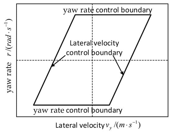 Figure 5. Schematics of envelope constraint of vehicle swing.
 - In order to achieve the required lateral tracking accuracy and control stability, the steering angle and the physical characteristics of the driving and braking should be considered. Apply the following constraints to the vehicle’s variables:where are the control input and control input increment of the trajectory tracking control system.
4.2. Trajectory Tracking Controller Based on MPC
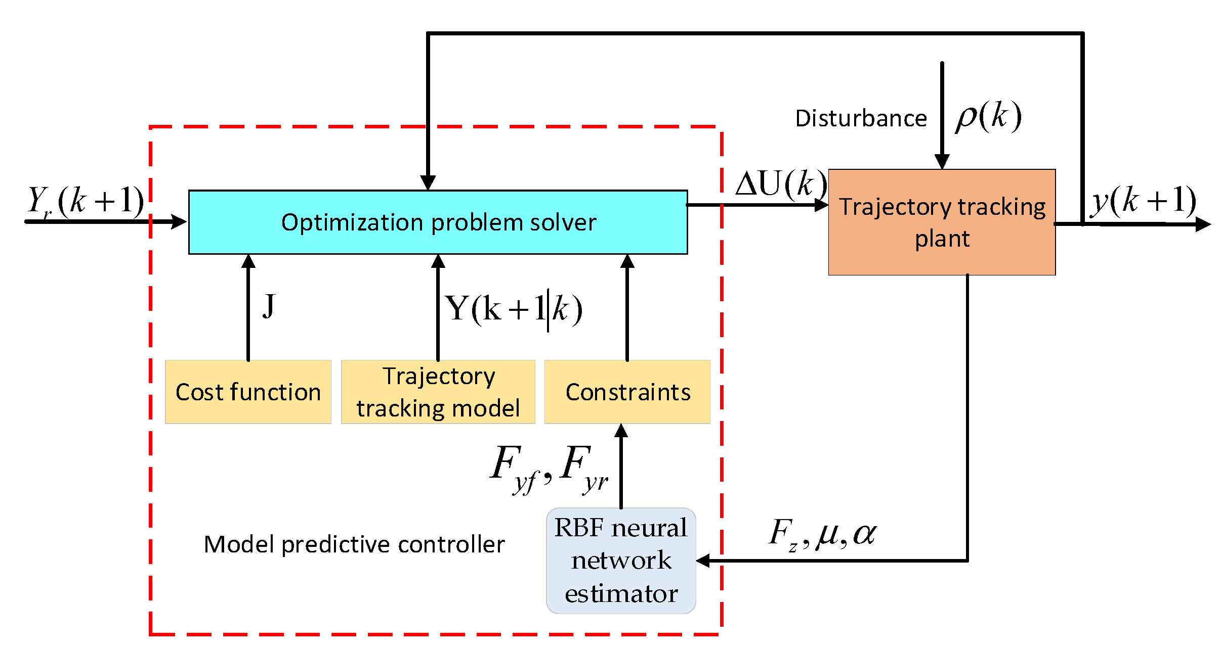
The function of the proposed trajectory tracking control system is to calculate the dynamic control command and subsequently manipulate the vehicle to the desired trajectory. This function is achieved with the control law and can be translated into solving an MPC problem. The schematic block diagram of the MPC algorithm is shown in Figure 6.
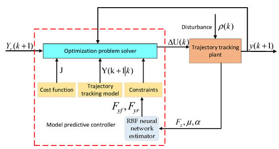
Figure 6.
Schematic block diagram of the proposed MPC algorithm.
During the transitional state, the reference is described as the control objective , and the disturbances are the road curvature and the desired longitudinal acceleration. The output is the lateral velocity, yaw rate, heading error and longitudinal velocity error. The MPC controller consists of three parts: the constraints, the trajectory tracking control model, and the cost function. The trajectory tracking model is designed according to the Equation (11). The constraints are shown in Equations (16)–(18).
To facilitate the design of the controller, the state vector and the input increment are usually coupled in a broadening vector that can be expressed as . Rewriting Equations (13) and (14):
where , Nx is the dimension of the state quantity and Nu means the dimension of the control quantity, and the change of the control input is . The predicted output performance vector and the sequence of the future incremental inputs at time step are denoted as and , respectively.
where is the prediction horizon and means the control horizon, are the predictive performance at the step , are the control input increments for the control time domain.
The MPC controller can predict the state of the next moment according to the state of the current moment, so the prediction equation can be expressed as:
The output vector of the predictive can be expressed in matrix form:
where , ,
.
To calculate the desired control increment, the trajectory tracking problem is converted to solve the quadratic optimal solution problem:
where is the weight matrix; and is the coefficient of relaxation. Combining Equation (20) with Equation (22), and defining , the objective function can be transformed into a quadratic optimization problem combined with the constraints and the following optimization problems can be solved:
where , .
In addition, Equations (12) and (20) transform the slip constraint (16) into a constraint on the control increment :
where, .
4.3. Lower-level Controller Design
In order to verify the effectiveness of the proposed MPC control algorithm, the lower-level controller needs to be established to convert the output of the MPC controller into the input of the actuator [36]. Among them, the control input of the steering system of the actuator is the front-wheel steering angle, and the control input of the driving system is the desired throttle opening and the desired braking master cylinder pressure . The schematic is shown in Figure 7. The switching logic of the lower-level controller can be simplified to compare with 0, to apply the drive control (drive mode) when , to compare the desired throttle opening with the throttle opening threshold and to carry out the PI control. Otherwise, the braking control (braking mode) is applied to compare the desired braking master cylinder pressure with the braking master cylinder pressure threshold and carry out the PI control. The switching logic can be formulated as:
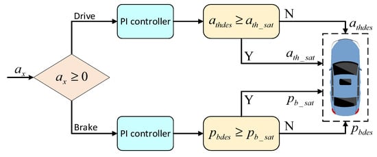
Figure 7.
Lower-level controller implementation block diagram.
5. Experimental Platform and Testing
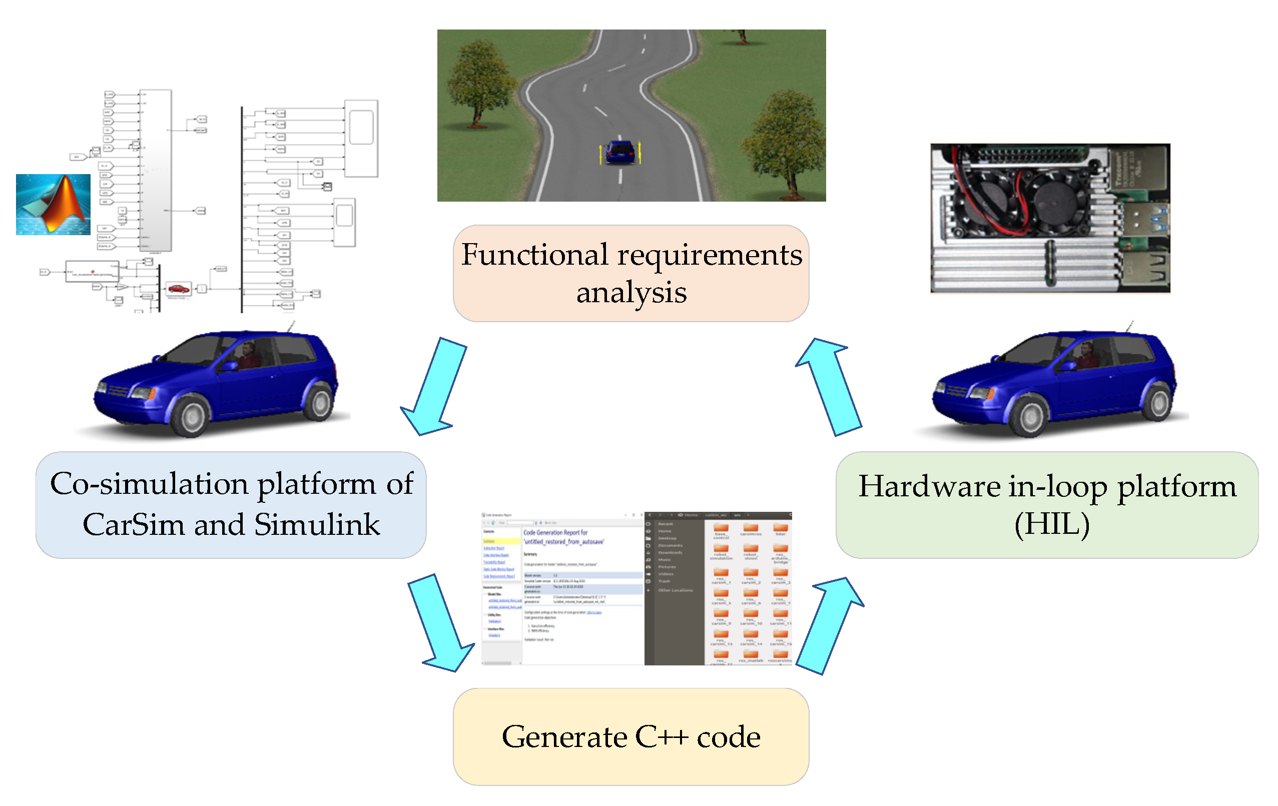
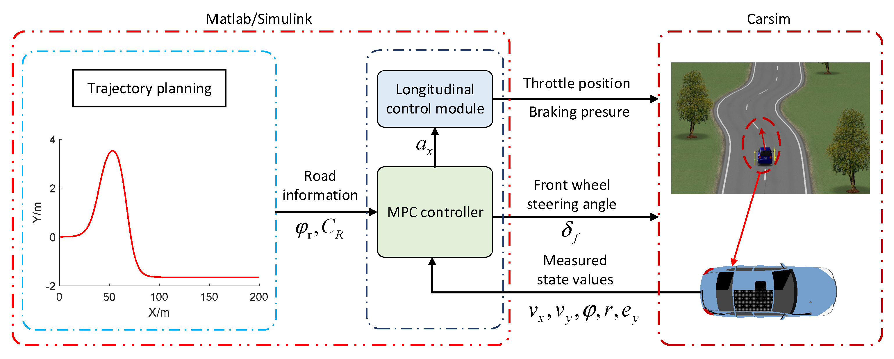
In order to fully demonstrate the advantages of the proposed control algorithm, the double-shift line condition is used as the test environment and builds a co-simulation performed of CarSim and Matlab/Simulink and the HIL platform. The development process is shown in Figure 8. Firstly, the functional analysis of the trajectory tracking system is carried out; secondly, the effectiveness of the MPC algorithm is verified by the co-simulation environment; thirdly, the MPC controller is compiled into the Raspberry Pi through the method of generating C++ code by Matlab, and the Raspberry Pi is used as a controller to control the controlled vehicle of the CarSim. CarSim, as a simulation software for vehicle dynamics, utilizes detailed vehicle characteristic parameters to simulate the dynamic behavior of vehicles and is widely used in the development of modern automotive control systems.
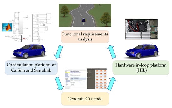
Figure 8.
Development process.
5.1. Simulation
In order to verify the validity of the proposal control algorithm, this section combines the virtual vehicle in CarSim software with the controller proposed in Matlab/Simulink to achieve trajectory tracking. The block diagram of the co-simulation is shown in Figure 9, and the primary parameters of the co-simulation are shown in Table 1.
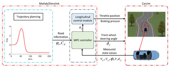
Figure 9.
Co-simulation block diagram.

Table 1.
Symbol and definition of parameters.
Furthermore, the RESM performance index was introduced to determine quantitative differences between the plotted data, and the RMSE is formulized as follows:
where is the predicted value at the time , is the true value at the time .
5.1.1. Accuracy of RBF Neural Network in Estimating Lateral Force
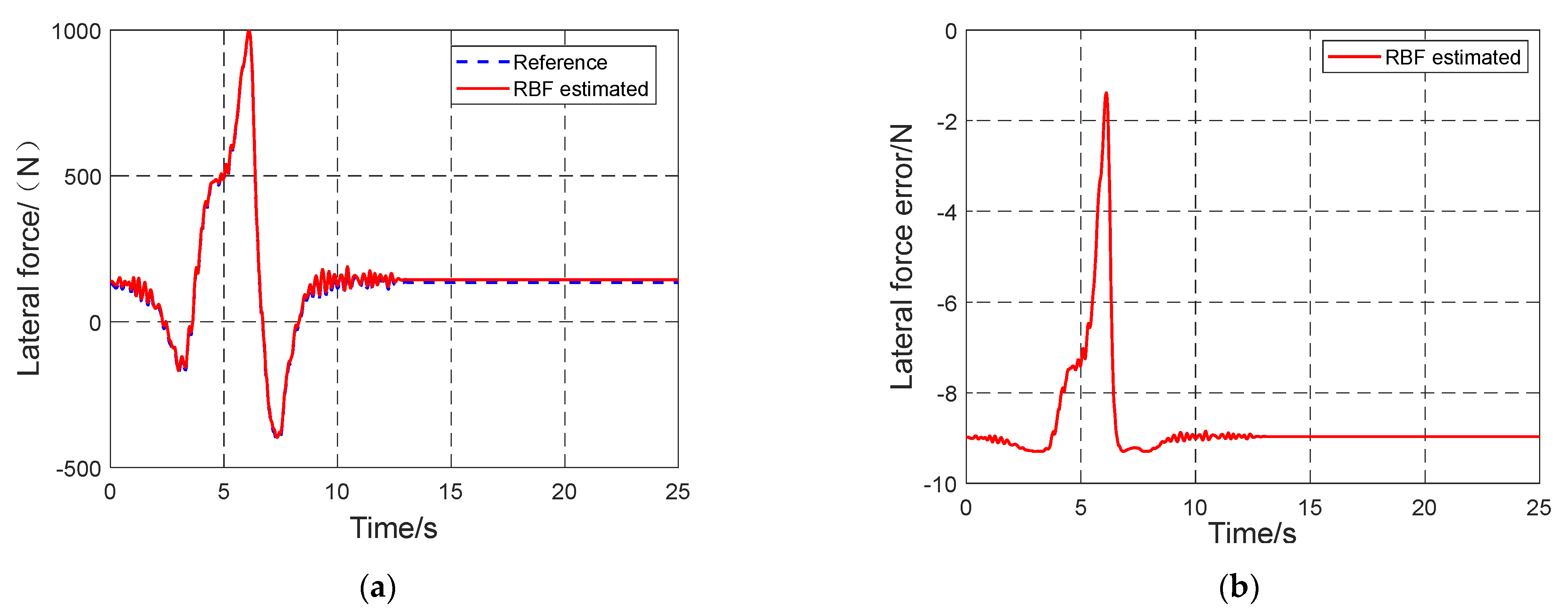
In order to verify the accuracy of the proposed RBF neural network in estimating lateral force, we carried out simulation experiments on ice-covered pavement, and set the adhesion coefficient of the ice-covered pavement to 0.3. The double-shift line condition was tested at , and the experimental results are shown in Figure 10. The error between the RBF neural network estimate and the true value of the tire is within 9N as shown in Figure 10. The RESM performance index between the RBF neural network estimate and the true value of the tire is 7.1473, which can effectively estimate the lateral force and apply it to the boundary value of the vehicle nonlinear dynamics model and slip constraint.
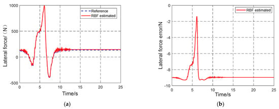
Figure 10.
Estimation results based on RBF neural network tire lateral force under ice-covered pavement; (a) The lateral force; (b) Discrepancy between the estimated lateral force and the true value.
5.1.2. Influence of Slip Constraints
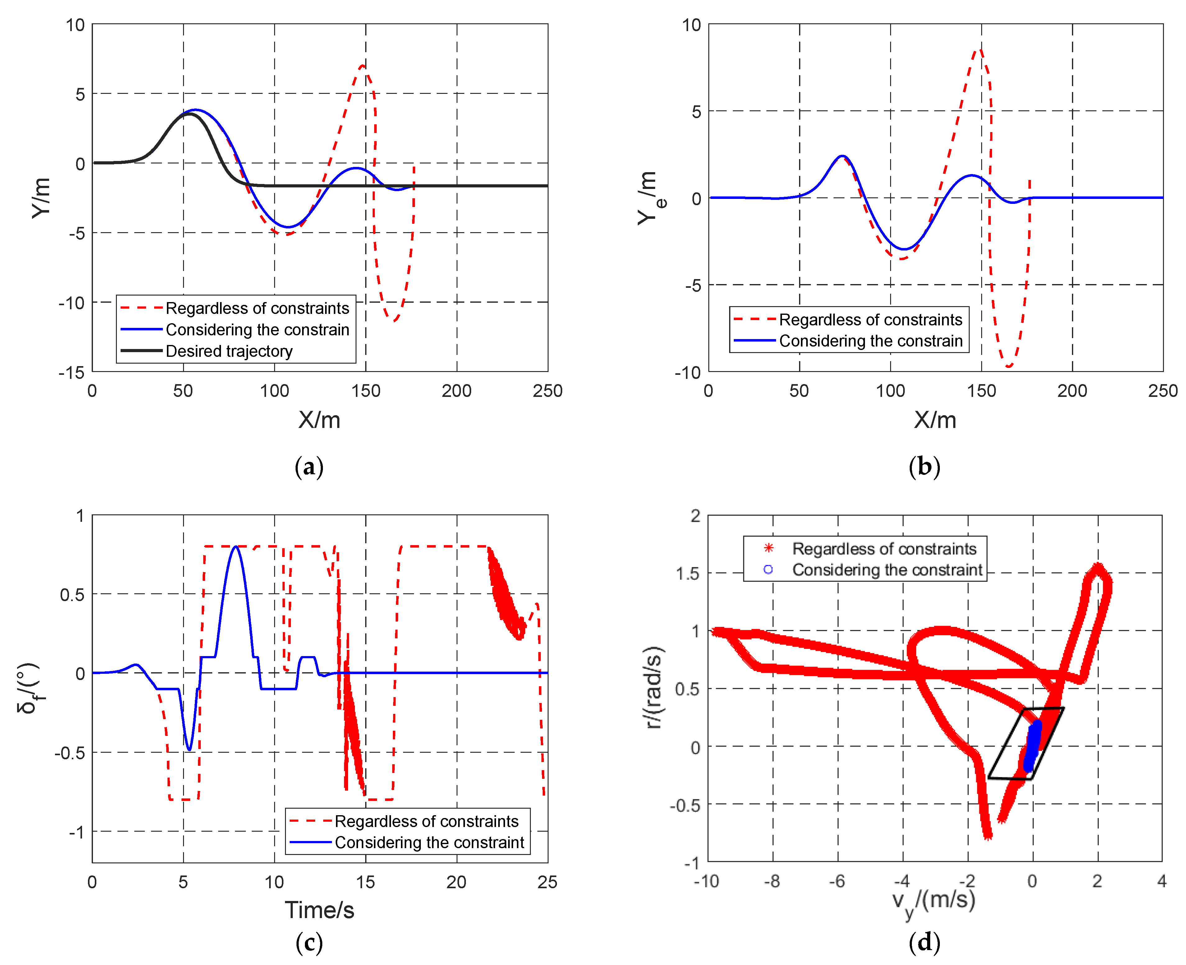
In order to verify the influence of the proposed algorithm on the operation stability of autonomous vehicles at the vehicle’s handling limits, we carried out simulation experiments on ice-covered pavement, and set the adhesion coefficient of the ice-covered pavement to 0.3. We compared applying the slip constraint and not applying the slip constraint at , and the experimental results are shown in Figure 11. Table 2 shows the RSME of the trajectory tracking error on the ice-covered pavement, and Figure 11 shows the results of the trajectory tracking and the comparison of the lateral velocity and yaw rate under the ice-covered pavement. Figure 11a,b show the vehicle has a serious skidding phenomenon at when no slipping constraint was imposed, and the vehicle can still drive effectively when the slip constraint is applied. As shown in Table 2, when the vehicle is in the slip constraint, the tracking performance of the desired trajectory is better, where the RESM of the trajectory tracking error is 0.9406; the front-wheel steering angle under the slip constraint is within the saturation constraint of the actuator as shown in Figure 11c. As shown in Figure 11d, the vehicle seriously exceeds the envelope constraint without the envelope constraint, and the vehicle becomes unstable. In summary, it can be seen that the application of the slip constraint can effectively improve the slip phenomenon of the vehicle and the vehicle is guaranteed to be within the envelope constraint.
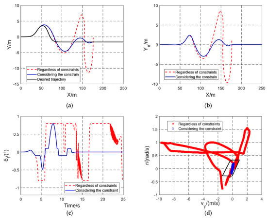
Figure 11.
Simulation results of ice-covered pavement trajectory tracking at ; (a) Trajectory tracking results; (b) Lateral tracking error; (c) The front-wheel steering angle; (d) Comparison of the lateral velocity and yaw rate under whether slip constraints are applied.

Table 2.
RMSE of trajectory tracking error on ice-covered pavement.
5.1.3. Effect of Nonlinear Envelope Constraints
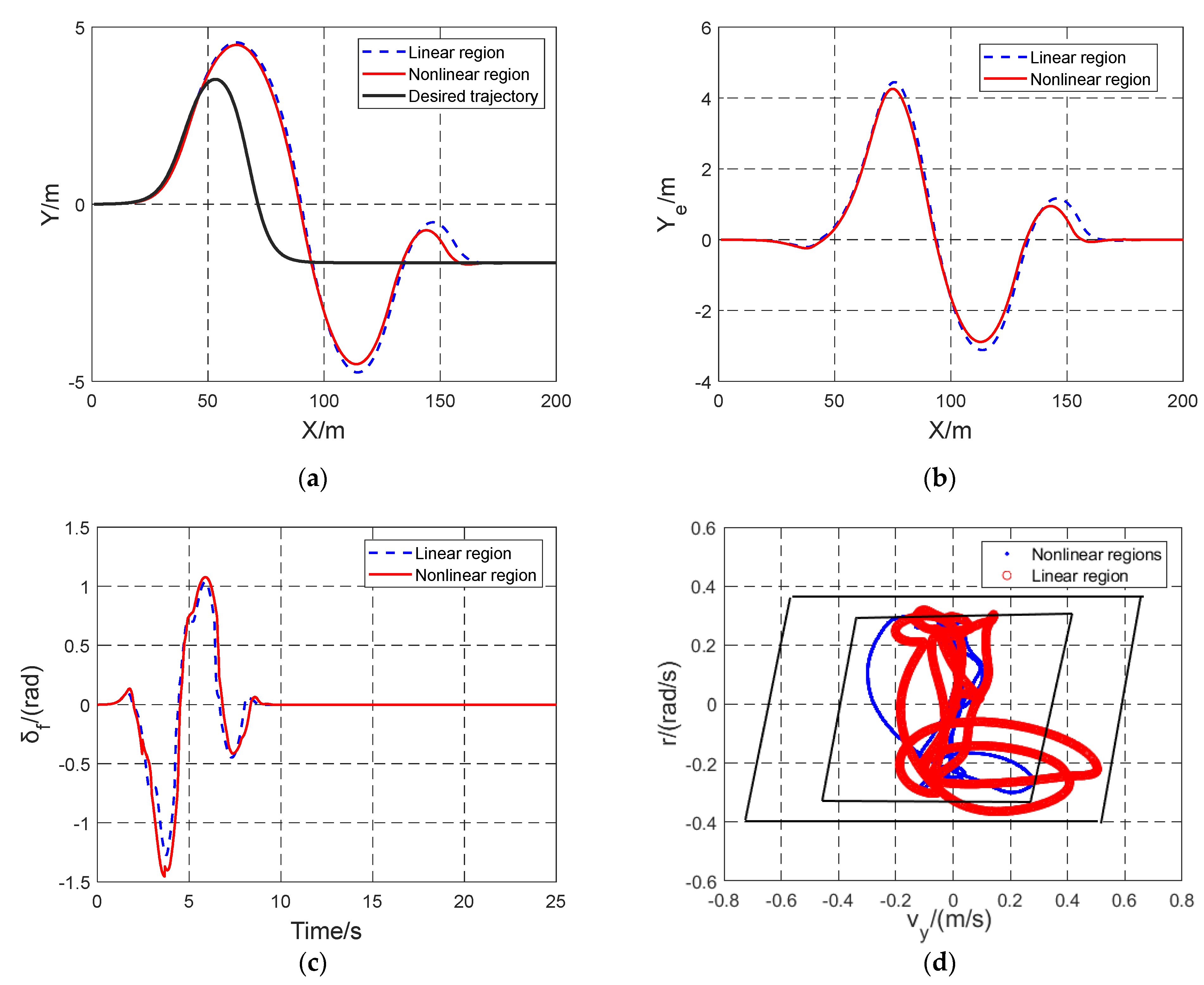
The algorithm proposed for verification can still ensure the driving of the vehicle beyond the nonlinear area of the tire. We carried out the simulation experiments on wet asphalt pavement and set its pavement adhesion coefficient to 0.6. We compared applying the slip constraint and not applying the slip constraint at . Figure 12 shows the results of the experiment. Figure 12 shows the results of the trajectory tracking and the comparison of the lateral velocity and yaw rate under the ice-covered pavement. The vehicle can still drive efficiently beyond the linear region, as shown in Figure 12a,b, and the tracking error of applying the nonlinear envelope constraint is smaller than the error of applying the linear envelope in the second half of the trajectory. As shown in Table 3, the nonlinear envelope constraint performed well in tracking the desired trajectory, where the RESM of the trajectory tracking error is 1.0886. The front-wheel steering angle is within the saturation constraint of the actuator as shown in Figure 12c. As shown in Figure 12d, the vehicle is constrained beyond the linear envelope and within the nonlinear envelope constraint, and the vehicle remains stable. In summary, it can be seen that the vehicle is within the constraint of the nonlinear envelope, and the vehicle can still drive effectively.
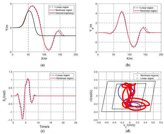
Figure 12.
Simulation results of wet asphalt pavement trajectory tracking at ; (a) Trajectory tracking results; (b) Lateral tracking error; (c) The front-wheel steering angle; (d) Comparison of the lateral velocity and yaw rate under whether slip constraints are applied.

Table 3.
RMSE of trajectory tracking error.
5.1.4. Comparison of Simulation Result
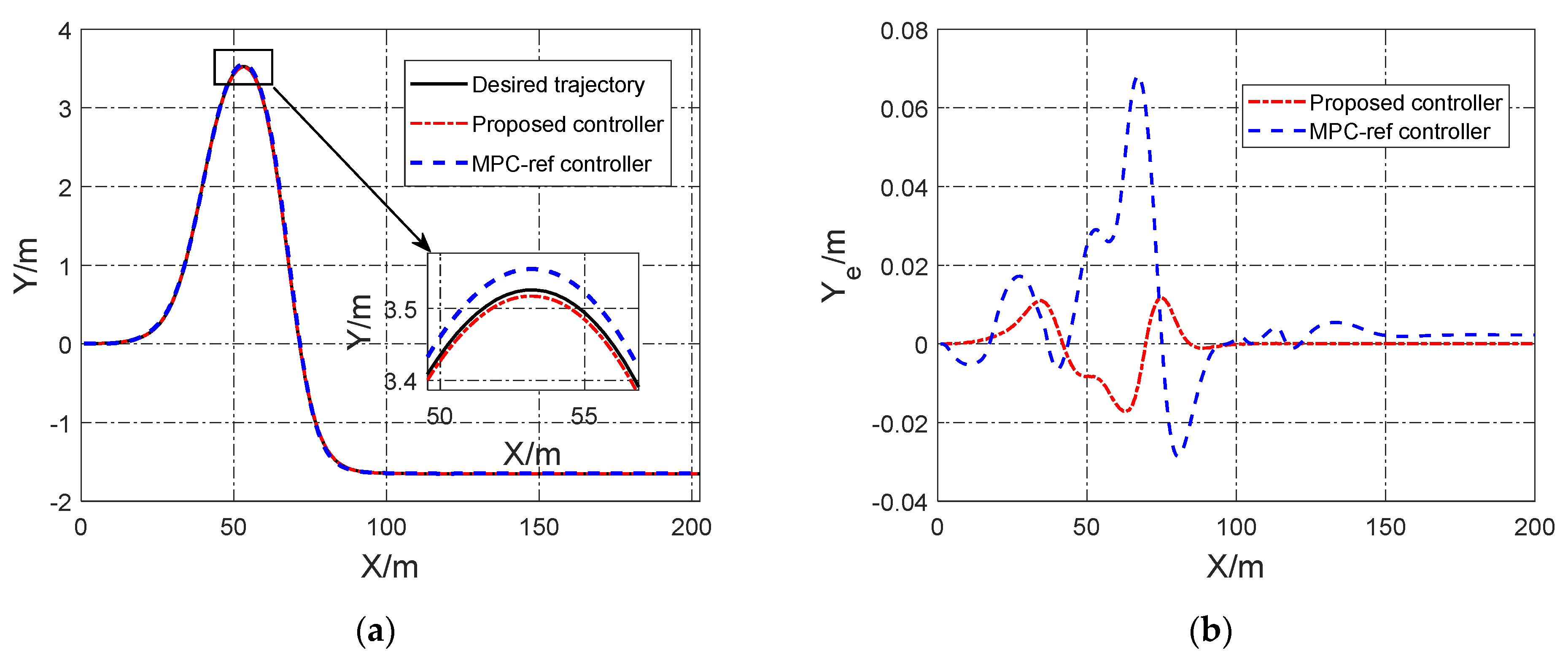
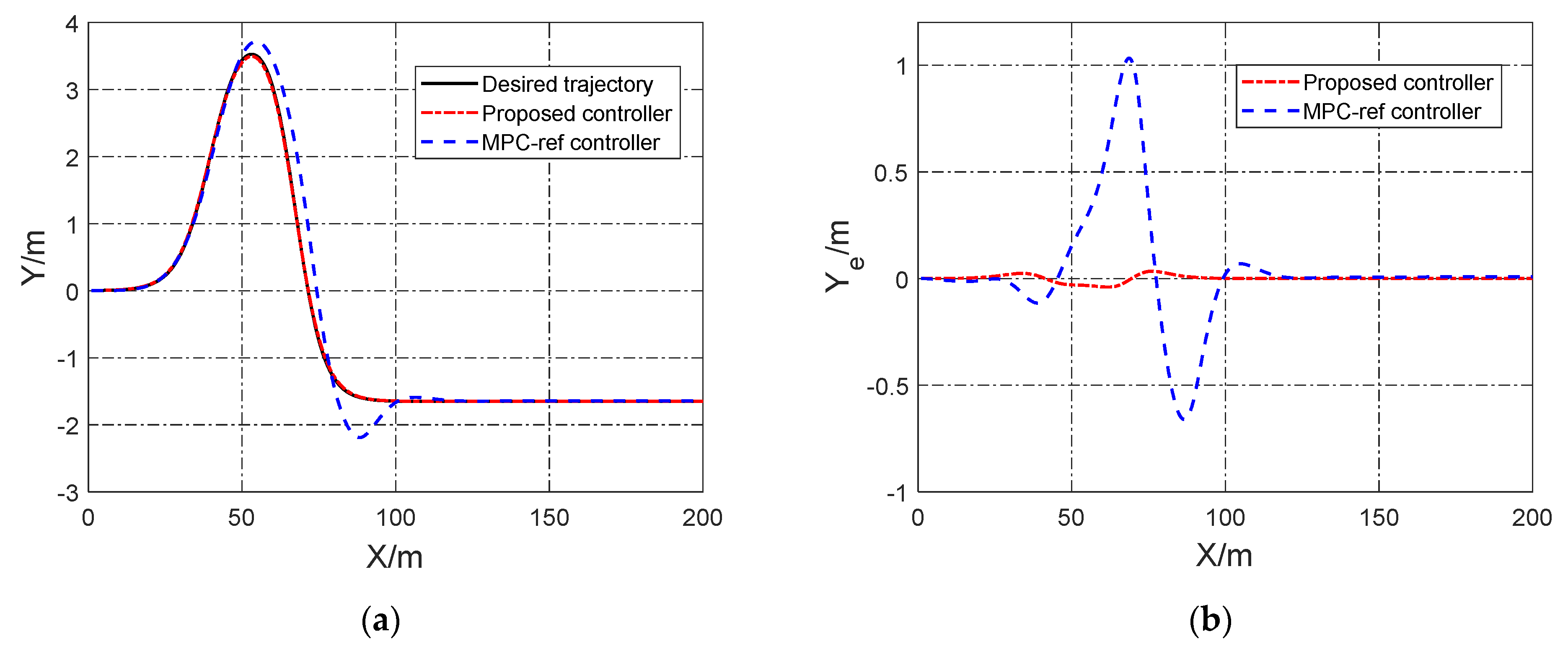
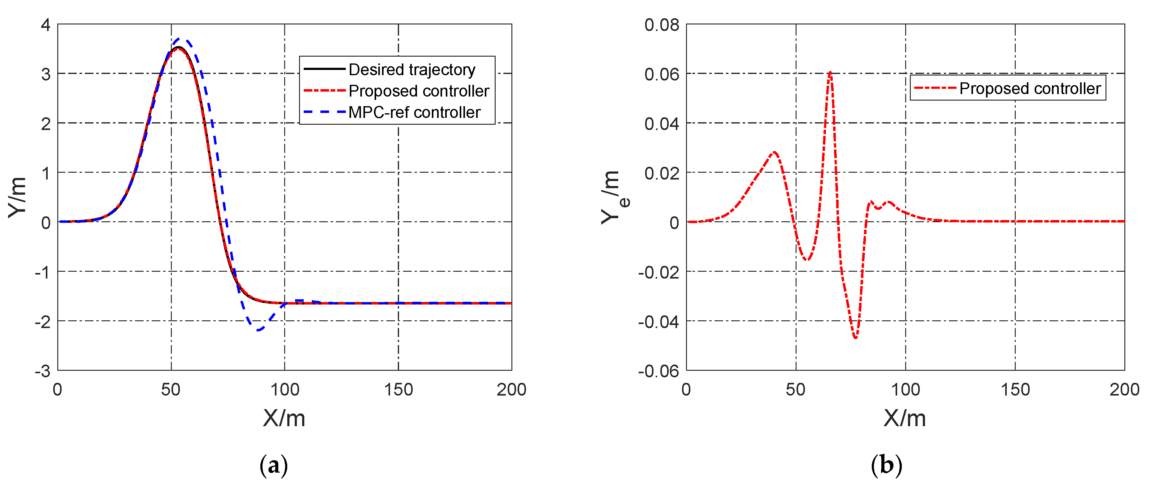
This section offers a comparison with the MPC trajectory tracking algorithm proposed in the Ref. [34]. In the first scenario, the vehicle has a driving speed of in the double-shift line condition as shown in Figure 13. In the second scenario, the vehicle has a driving speed of in the double-shift line condition as shown in Figure 14. In the third scenario, the vehicle has a driving speed of in the double-shift line condition as shown in Figure 15. The RESM of the trajectory tracking error as shown in Table 4.
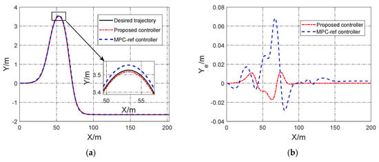
Figure 13.
Trajectory tracking results compared to the algorithm proposed at 36; (a) Comparison of driving paths; (b) Comparison of lateral errors.
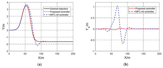
Figure 14.
Trajectory tracking results compared to the algorithm proposed at ; (a) Comparison of driving paths; (b) Comparison of lateral errors.
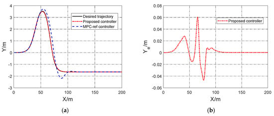
Figure 15.
Trajectory tracking results at ; (a) Driving path; (b) Lateral tracking error.

Table 4.
RESM of the trajectory tracking error.
As shown in Figure 13a, the algorithm proposed in Ref. [34] and the algorithm proposed in this paper effectively track the desired trajectory at . Moreover, the tracking error of the algorithm proposed can be maintained within the range of 0.04 m. The tracking error of the Ref. is within as shown in Figure 13b, but it is still large compared to the algorithm proposed. When the driving speed is , Ref. [34] has a large tracking error, and the algorithm proposed still maintains a good control effect, and the tracking error is maintained in the range of 0.05m, as shown in Figure 14. As shown in Figure 15, the algorithm proposed can effectively track the desired trajectory, and the tracking error remains within 0.07 m. Compared with the algorithm proposed in Ref. [34], the proposed controller performed well in tracking the desired trajectory, as shown in Table 4. The effectiveness of the trajectory tracking controller proposed is effectively verified, and it can be tracked at higher speeds compared with Ref. [34].
5.2. Hardware-in-loop Platform and Test
5.2.1. Desired Trajectory Setting
The quintile polynomial curve fitting can plan a trajectory with a smooth curvature according to the initial and final states of the vehicle, which is widely used in trajectory tracking. The time-based quintile polynomial curve fitting generates the desired trajectory, and it verifies the effectiveness of the MPC trajectory tracking controller through the Raspberry Pi. The quintile polynomial curve fitting can be described as:
where , are designed according to the initial and final state of the vehicle.
The calculation formula for the heading angle and the curvature road is as follows:
5.2.2. Hardware-in-loop Platform Setup
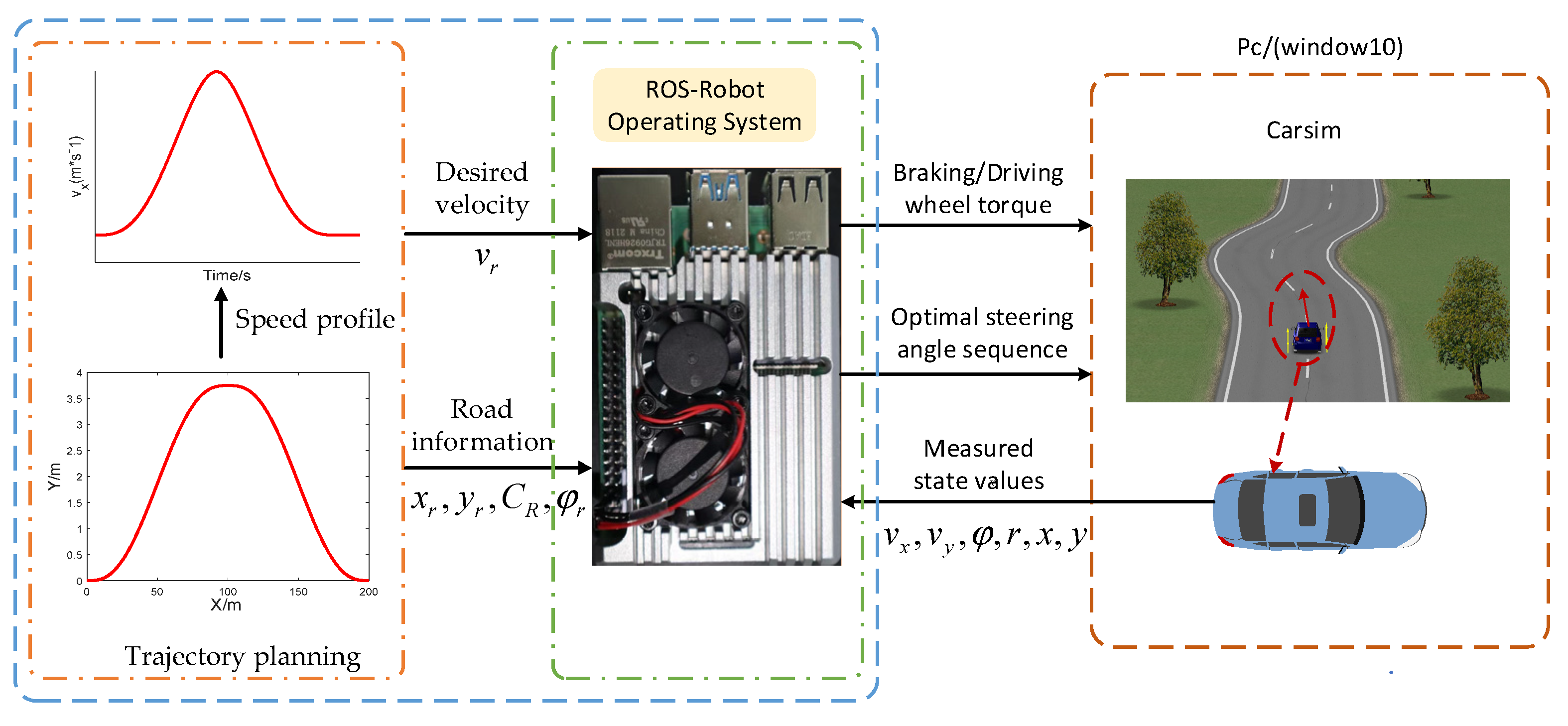
In the hardware-in-loop platform design, the Robot Operating System (ROS) system is used as a platform for the operation of the vehicle program, and the MPC trajectory tracking program runs in ROS. As an alternative to a physical car, has the same object characteristics as a physical car. In addition, implements the information transfer between and ROS through topic communication. ROS (MPC trajectory tracking program) obtains the status information of the vehicle: the vehicle position, acceleration, yaw angle and yaw rate, and the quintile polynomial curve fitting to calculate the desired trajectory information and processes, and it calculates that information and obtains the feedback information at the current moment, such as the vehicle’s desired throttle opening, the desired brake master cylinder pressure, and the front-wheel steering angle, where this feedback control information is simultaneously communicated to CarSim (vehicle) to control the vehicle in real time. The control block diagram is shown in Figure 16.
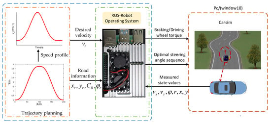
Figure 16.
Hardware-in-loop platform.
ROS runs on the Raspberry Pi 4B (CPU 64bit 1.5 GHz, 8 GB Sto-rage) with the ubuntu18.4+ros melodic system, and CarSim runs on the same computer as Matlab (CPU i9-10850k 3.60 GHz). The control cycle of ROS (MPC trajectory tracking program) is = . Four scenarios (low speed, medium speed, medium-high speed, and high speed) are set to verify the effectiveness of the proposed algorithm. The primary parameters of the simulated vehicle are shown in Table 1.
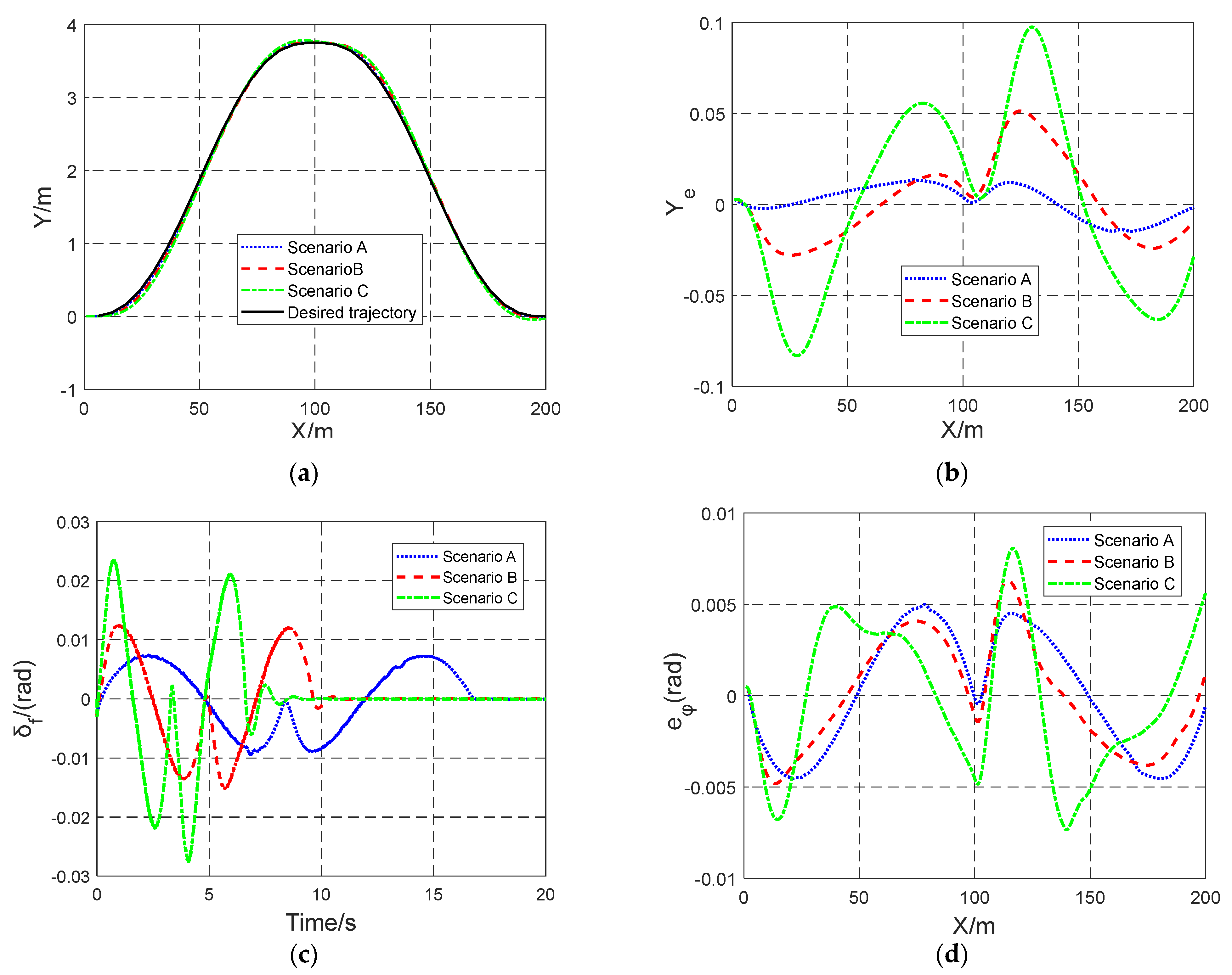
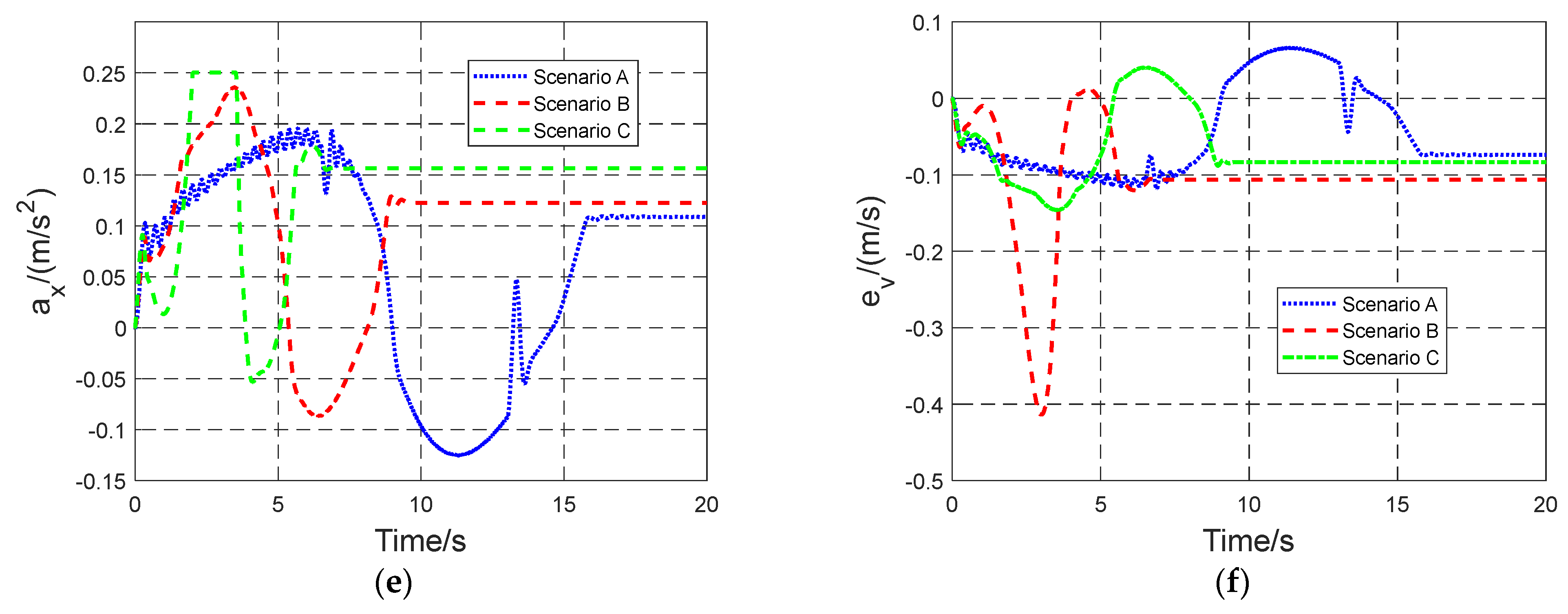
In the first scenario, the vehicle enters the desired trajectory at an initial velocity of 36 km/h, reaches the center point of the desired trajectory at a speed of 54 km/h, and then reaches the end of the desired trajectory to return to the initial speed and continue driving at the initial speed. The description of the other three scenes is similar to the first. The information for the four scenario is shown in Table 5. Scenario A, B, C, and D represent the first, second, third, and fourth scenario, respectively.

Table 5.
Simulation scenarios.
5.2.3. Hardware-in-loop Platform Results and Analysis
In this hardware-in-loop platform experiment, dry asphalt pavement was selected and the adhesion coefficient was set to 0.75. Table 6 shows the RMSE of trajectory tracking error under the three scenarios. The results of the trajectory tracking under the three scenarios are displayed in Figure 17. Figure 17a,b show that the lateral deviation of unmanned vehicles is always kept within 0.10 m, where the control effect is good under the three scenarios. The lower the velocity, the lower the tracking error. As shown in Table 6, the RMSE of trajectory tracking error is always kept within 0.0430, and the lower the velocity, the smaller the RMSE of the tracking error. Figure 17c shows that the front-wheel steering angle optimized by the controller is within the saturation constraint of the actuator regardless of the velocity. The three scenario errors are small and have better tracking performance as shown in Figure 17d. Figure 17e shows that the longitudinal acceleration of the vehicle is much less than 0.2 g and is always within the saturation constraint. Figure 17f shows that the longitudinal velocity error of the vehicle is 0.15 m/s and has good tracking performance in the two scenarios of Scenario A and Scenario B, but the longitudinal velocity error in Scenarios C is within 0.35 m/s, and the longitudinal velocity error is large.

Table 6.
RMSE of trajectory tracking error in the three scenarios.
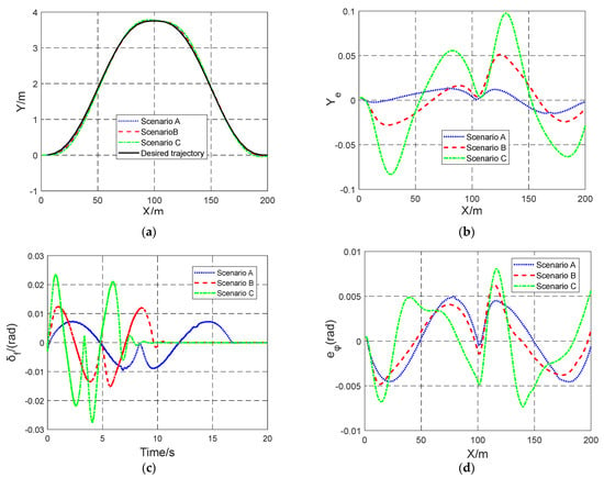
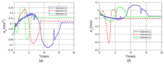
Figure 17.
The simulation results of trajectory tracking: (a) Driving paths; (b) Lateral error; (c) The front-wheel steering angle; (d) The heading error; (e) Longitudinal acceleration; (f) Longitudinal velocity error.
5.2.4. Comparative Analysis of Co-simulation and Hardware-in-loop Platform Experiments
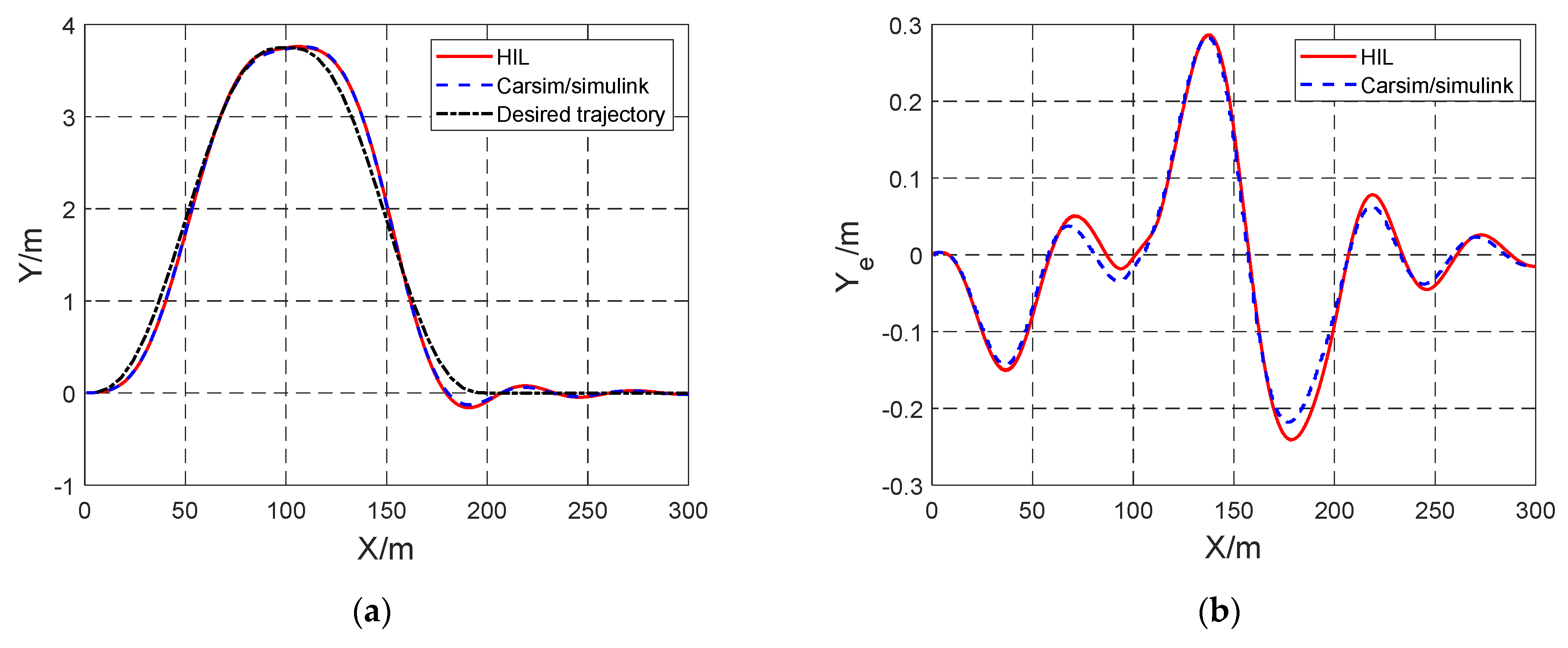
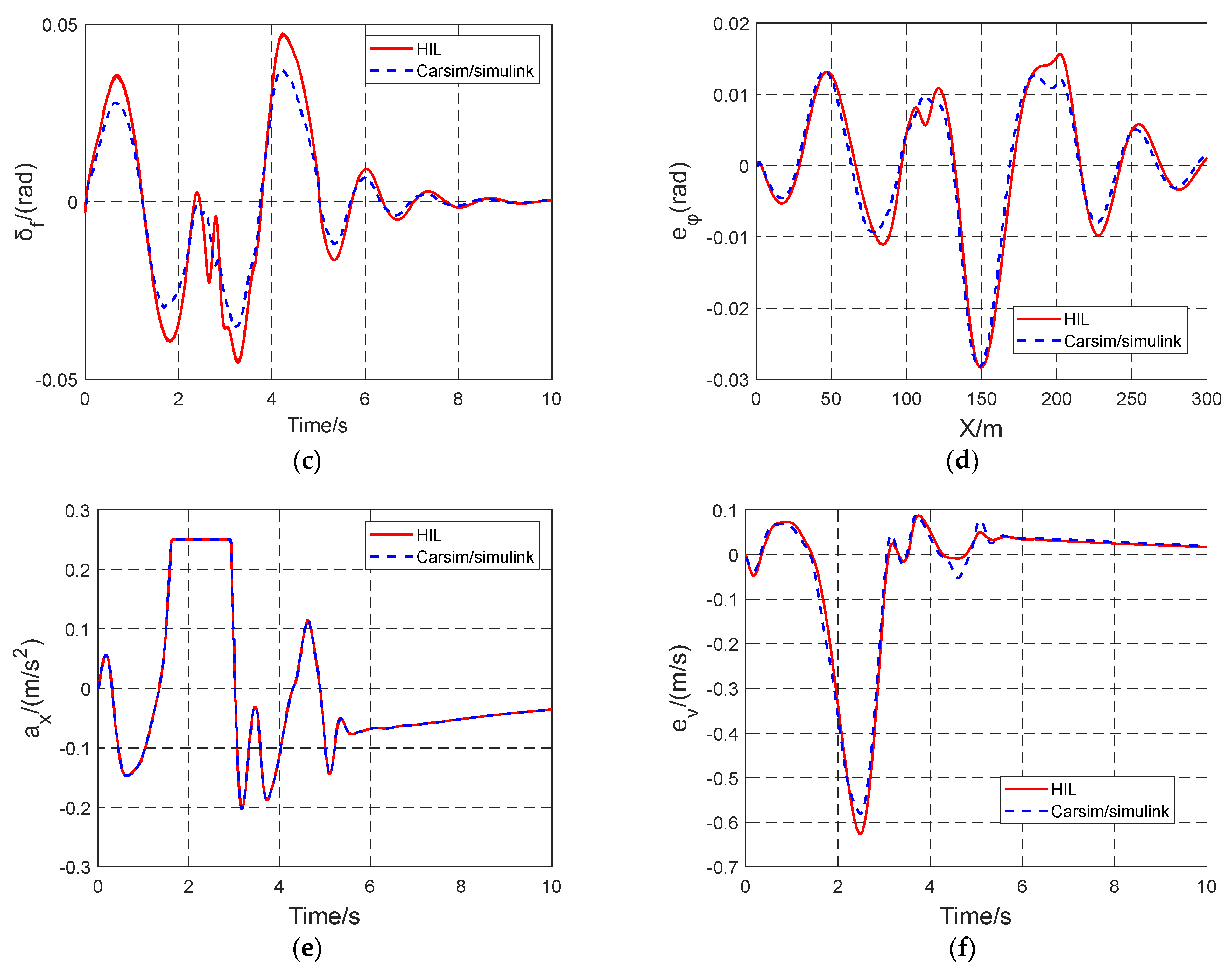
The comparison verification is carried out in Scenario D, where the dry asphalt pavement was selected and the adhesion coefficient was set to 0.75; the results are shown in Figure 18. The RMSE of the trajectory tracking error is shown in Table 7. The results show that the controller proposed in this paper achieves good control effects in both CarSim/Simulink co-simulation and the HIL platform. However, the front-wheel steering angle in the HIL platform is higher than that in co-simulation as shown in Figure 18c. The longitudinal velocity error of the HIL simulation is larger, as shown in Figure 18f. What is more, the co-simulation performed well in tracking the desired trajectory, where the RESM of the trajectory tracking error is 0.0667, as shown in Table 7.
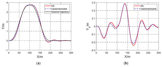

Figure 18.
Trajectory tracking simulation results at Scenario D: (a) Driving paths; (b) Lateral error; (c) The front-wheel steering angle; (d) The heading error; (e) Longitudinal acceleration; (f) Longitudinal velocity error.

Table 7.
RMSE of trajectory tracking error in Scenario D.
6. Conclusions
In this paper, a control law is designed to improve the trajectory tracking accuracy and vehicle handling stability to achieve safe driving. The control law is based on the model predictive control with the slip constraint, which calculates the desired longitudinal acceleration and the desired front-wheel steering angle. In addition, the proposed control law can satisfy such control objectives and the vehicle handling stability simultaneously during the control period. The research is summarized below:
- In order to improve the tracking accuracy of the vehicle and the stability of the vehicle, a control method, which considers the influence of road curvature and tire nonlinear dynamic characteristics on the trajectory tracking performance, is developed by the control law based on the MPC. Furthermore, the lateral force is estimated based on the RBF neural network, which is incorporated into the boundary conditions of the vehicle envelope constraint to reduce the slip phenomenon of vehicles;
- The trajectory tracking control system with the control law is simulated by Matlab/Simulink and Raspberry Pi combined with the CarSim-based vehicle model. Meanwhile, the development technology route was expounded;
- In co-simulation (CarSim/Simulink), the accuracy of the RBF neural network in estimating the lateral force is verified under actual driving conditions; the slip phenomenon can be effectively reduced after the vehicle is applied to the envelope constraint; and the influence of the vehicle on the driving state after the linear and nonlinear envelope constraint is analyzed. Finally, compared with the Ref. [34], the results show that the proposed controller is better than the controller proposed in the Ref. [34];
- In the HIL platform, we verify the performance of the proposed MPC controller in three different scenarios. Finally, in comparing the co-simulation results with the HIL platform, the results show that the co-simulation is better than the HIL platform;
- In the future research, the study of the tire deflection characteristics based on experimental data would be considered. In addition, on the basis of the establishment of the HIL platform, the ROS-based verification platform is built to verify the effectiveness of the proposed algorithm.
Author Contributions
Conceptualization, Y.L., T.Y. and R.Z.; methodology, Y.L., T.Y. and R.Z.; validation, Y.L., T.Y. and R.Z.; formal analysis, Y.L., T.Y. and R.Z.; investigation, Y.L., T.Y. and R.Z.; resources, Y.L., T.Y. and R.Z.; writing—original draft preparation, Y.L., T.Y. and R.Z.; writing—review and editing, Y.L., T.Y. and R.Z.; supervision, R.Z.; project administration, Y.L.; funding acquisition, R.Z. All authors have read and agreed to the published version of the manuscript.
Funding
This work was funded by the Cooperation Project of Guizhou Education Department (Grant Number KY [2021] 297), the Science and Technology Foundation of Guizhou Province (Grant Number ZK [2021] 320), the M.S. Research Project Foundation of Guizhou Province (Grant Number YJSKYJJ [2021] 101), and the Ph.D. Research Project of Guizhou Normal University (Grant Number GZNUD [2019] 22).
Institutional Review Board Statement
Not applicable.
Informed Consent Statement
Not applicable.
Data Availability Statement
The data presented in this study are available on request from the corresponding author.
Acknowledgments
The authors gratefully acknowledge the contribution from School of Mechanical and Electrical Engineering, Guizhou Normal University.
Conflicts of Interest
The authors declare no conflict of interest.
Abbreviations
The following abbreviations and symbols are used in this paper:
| Symbol | Description |
| Coordinates of center of gravity (CG) | |
| (rad) | Yaw angle of vehicle body |
| (rad/s) | Yaw rate of vehicle body |
| (m/s) | Longitudinal/lateral velocity |
| Offset of CG from the reference point | |
| (rad) | Orientation error of yaw angle with respect to the desired trajectory |
| Error between the current and the desired longitudinal velocity | |
| (kg) | Vehicle mass |
| Yaw moment of inertia of the vehicle | |
| (m) | Distance from CG to the front/real axle |
| Longitudinal tire force of the front/rear wheel | |
| Lateral tire force of the front/rear wheel | |
| Vertical load | |
| Cornering stiffness of the front wheel | |
| Cornering stiffness of the real wheel | |
| Slip angle of the front/ rear wheel | |
| Longitudinal acceleration of vehicle | |
| (rad) | Front-wheel steering angle |
| Road curvature | |
| Road friction coefficient | |
| Center width of the hidden layer | |
| X | Input vector for RBF neural network |
| Central unit of the jth radial basis function | |
| Weight for RBF neural network | |
| (s) | Sampling time |
| Weight matrix for MPC | |
| Coefficient of relaxation | |
| Desired throttle opening | |
| Desired braking master cylinder pressure | |
| Throttle opening threshold | |
| Expected braking main cylinder pressure | |
| Predicted value for RESM | |
| True value for RESM | |
| MPC | Model prediction control |
| RBF | Radial basis function |
| PID | Proportional-integrated-differential |
| LQR | Linear quadratic regulator |
| SMC | Sliding mode control |
| ZOH | Zero-order retention |
| CarSim | A simulation software specifically for vehicle dynamics |
| Simulink | A modular diagram environment for multidomain simulation as well as model-based design |
| RMSE | Root mean square error |
| UKF | Unscented Kalman Filter |
| PWA | Piecewise affine |
| HIL | Hardware-in-loop |
| ROS | Robot Operating System |
| CG | Center of gravity |
References
- Schwarting, W.; Alonso-Mora, J.; Rus, D. Planning and Decision-Making for Autonomous Vehicles. Annu. Rev. Control Robot. Auton. Syst. 2018, 1, 187–210. [Google Scholar] [CrossRef]
- Wang, H.; Wang, Q.; Chen, W.; Zhao, L.; Tan, D. Path Tracking Based on Model Predictive Control with Variable Predictive Horizon. Trans. Inst. Meas. Control 2021, 43, 2676–2688. [Google Scholar] [CrossRef]
- Yang, H.; Wang, Z.; Xia, Y.; Zuo, Z. EMPC with Adaptive APF of Obstacle Avoidance and Trajectory Tracking for Autonomous Electric Vehicles. ISA Trans. 2022, S001905782200475X. [Google Scholar] [CrossRef]
- Gao, L.; Beal, C.; Mitrovich, J.; Brennan, S. Vehicle Model Predictive Trajectory Tracking Control with Curvature and Friction Preview. IFAC-Pap. 2022, 55, 221–226. [Google Scholar] [CrossRef]
- Yue, M.; An, C.; Sun, J. Zero Dynamics Stabilisation and Adaptive Trajectory Tracking for WIP Vehicles through Feedback Linearisation and LQR Technique. Int. J. Control 2016, 89, 2533–2542. [Google Scholar] [CrossRef]
- Park, M.; Kang, Y. Experimental Verification of a Drift Controller for Autonomous Vehicle Tracking: A Circular Trajectory Using LQR Method. Int. J. Control Autom. Syst. 2021, 19, 404–416. [Google Scholar] [CrossRef]
- Yang, L.; Yue, M.; Ma, T.; Hou, X. Trajectory Tracking Control for 4WD Vehicles Using MPC and Adaptive Fuzzy Control. In Proceedings of the 2017 36th Chinese Control Conference (CCC), Dalian, China, 26–28 July 2017; pp. 9367–9372. [Google Scholar]
- Xiong, B.; Qu, S. Intelligent Vehicle’s Path Tracking Based on Fuzzy Control. J. Transp. Syst. Eng. Inf. Technol. 2010, 10, 70–75. [Google Scholar] [CrossRef]
- Hwang, C.-L.; Yang, C.-C.; Hung, J.Y. Path Tracking of an Autonomous Ground Vehicle with Different Payloads by Hierarchical Improved Fuzzy Dynamic Sliding-Mode Control. IEEE Trans. Fuzzy Syst. 2018, 26, 899–914. [Google Scholar] [CrossRef]
- Bei, S.; Hu, H.; Li, B.; Tian, J.; Tang, H.; Quan, Z.; Zhu, Y. Research on the Trajectory Tracking of Adaptive Second-Order Sliding Mode Control Based on Super-Twisting. WEVJ 2022, 13, 141. [Google Scholar] [CrossRef]
- Marino, R.; Scalzi, S.; Orlando, G.; Netto, M. A Nested PID Steering Control for Lane Keeping in Vision Based Autonomous Vehicles. In Proceedings of the 2009 American Control Conference, St. Louis, MO, USA, 10–12 June 2009; pp. 2885–2890. [Google Scholar]
- Falcone, P.; Eric Tseng, H.; Borrelli, F.; Asgari, J.; Hrovat, D. MPC-Based Yaw and Lateral Stabilisation via Active Front Steering and Braking. Veh. Syst. Dyn. 2008, 46, 611–628. [Google Scholar] [CrossRef]
- Zhang, K.; Sun, Q.; Shi, Y. Trajectory Tracking Control of Autonomous Ground Vehicles Using Adaptive Learning MPC. IEEE Trans. Neural Netw. Learn. Syst. 2021, 32, 5554–5564. [Google Scholar] [CrossRef] [PubMed]
- Hu, J.; Xiong, S.; Zha, J.; Fu, C. Lane Detection and Trajectory Tracking Control of Autonomous Vehicle Based on Model Predictive Control. Int.J Automot. Technol. 2020, 21, 285–295. [Google Scholar] [CrossRef]
- Brown, M.; Funke, J.; Erlien, S.; Gerdes, J.C. Safe Driving Envelopes for Path Tracking in Autonomous Vehicles. Control Eng. Pract. 2017, 61, 307–316. [Google Scholar] [CrossRef]
- Alrifaee, B.; Maczijewski, J.; Abel, D. Sequential Convex Programming MPC for Dynamic Vehicle Collision Avoidance. In Proceedings of the 2017 IEEE Conference on Control Technology and Applications (CCTA), Mauna Lani Resort, HI, USA, 27–30 August 2017; pp. 2202–2207. [Google Scholar]
- Zhang, B.; Zong, C.; Chen, G.; Zhang, B. Electrical Vehicle Path Tracking Based Model Predictive Control with a Laguerre Function and Exponential Weight. IEEE Access 2019, 7, 17082–17097. [Google Scholar] [CrossRef]
- Tan, Q.; Dai, P.; Zhang, Z.; Katupitiya, J. MPC and PSO Based Control Methodology for Path Tracking of 4WS4WD Vehicles. Appl. Sci. 2018, 8, 1000. [Google Scholar] [CrossRef]
- Tang, L.; Yan, F.; Zou, B.; Wang, K.; Lv, C. An Improved Kinematic Model Predictive Control for High-Speed Path Tracking of Autonomous Vehicles. IEEE Access 2020, 8, 51400–51413. [Google Scholar] [CrossRef]
- Guo, N.; Zhang, X.; Zou, Y.; Lenzo, B.; Zhang, T. A Computationally Efficient Path-Following Control Strategy of Autonomous Electric Vehicles with Yaw Motion Stabilization. IEEE Trans. Transp. Electrific. 2020, 6, 728–739. [Google Scholar] [CrossRef]
- Banginwar, P.; Sands, T. Autonomous Vehicle Control Comparison. Vehicles 2022, 4, 59. [Google Scholar] [CrossRef]
- Raigoza, K.; Sands, T. Autonomous Trajectory Generation Comparison for De-Orbiting with Multiple Collision Avoidance. Sensors 2022, 22, 7066. [Google Scholar] [CrossRef]
- Chen, S.; Xiong, G.; Chen, H.; Negrut, D. MPC-Based Path Tracking with PID Speed Control for High-Speed Autonomous Vehicles Considering Time-Optimal Travel. J. Cent. South Univ. 2020, 27, 3702–3720. [Google Scholar] [CrossRef]
- Yu, H.; Duan, J.; Taheri, S.; Cheng, H.; Qi, Z. A Model Predictive Control Approach Combined Unscented Kalman Filter Vehicle State Estimation in Intelligent Vehicle Trajectory Tracking. Adv. Mech. Eng. 2015, 7, 557836. [Google Scholar] [CrossRef]
- Jeong, Y.; Yim, S. Integrated Path Tracking and Lateral Stability Control with Four-Wheel Independent Steering for Autonomous Electric Vehicles on Low Friction Roads. Machines 2022, 10, 650. [Google Scholar] [CrossRef]
- Fan, S.; Xie, T.; Chen, Z.; Hu, X.; Gao, L. Optimal Control of High Speed Unmanned Vehicle Path Tracking. J. Phys. Conf. Ser. 2022, 2195, 012006. [Google Scholar] [CrossRef]
- Chen, W.; Yan, M.; Wang, Q.; Xu, K. Dynamic Path Planning and Path Following Control for Autonomous Vehicle Based on the Piecewise Affine Tire Model. Proc. Inst. Mech. Eng. Part D J. Automob. Eng. 2021, 235, 881–893. [Google Scholar] [CrossRef]
- Mammar, S.; Enache, N.M.; Glaser, S.; Lusetti, B.; Neto, A.B. Lane Keeping Automation at Tire Saturation. In Proceedings of the 2010 American Control Conference, Baltimore, MD, USA, 30 June–2 July 2010; pp. 6466–6471. [Google Scholar]
- Chen, G.; Zhao, X.; Gao, Z.; Hua, M. Dynamic Drifting Control for General Path Tracking of Autonomous Vehicles. IEEE Trans. Intell. Veh. 2023, 1–12. [Google Scholar] [CrossRef]
- Chen, G.; Hua, M.; Zong, C.; Zhang, B.; Huang, Y. Comprehensive Chassis Control Strategy of FWIC-EV Based on Sliding Mode Control. IET Intelligent Transport Systems 2019, 13, 703–713. [Google Scholar] [CrossRef]
- Beal, C.E.; Gerdes, J.C. Model Predictive Control for Vehicle Stabilization at the Limits of Handling. IEEE Trans. Contr. Syst. Technol. 2013, 21, 1258–1269. [Google Scholar] [CrossRef]
- Xia, X.; Xiong, L.; Liu, W.; Yu, Z. Automated Vehicle Attitude and Lateral Velocity Estimation Using a 6-D IMU Aided by Vehicle Dynamics. In Proceedings of the 2018 IEEE Intelligent Vehicles Symposium (IV), Changshu, China, 26–30 June 2018; pp. 1563–1569. [Google Scholar]
- Liu, W.; Xia, X.; Xiong, L.; Lu, Y.; Gao, L.; Yu, Z. Automated Vehicle Sideslip Angle Estimation Considering Signal Measurement Characteristic. IEEE Sens. J. 2021, 21, 21675–21687. [Google Scholar] [CrossRef]
- Yang, K.; Tang, X.; Qin, Y.; Huang, Y.; Wang, H.; Pu, H. Comparative Study of Trajectory Tracking Control for Automated Vehicles via Model Predictive Control and Robust H-Infinity State Feedback Control. Chin. J. Mech. Eng. 2021, 34, 74. [Google Scholar] [CrossRef]
- Funke, J.; Brown, M.; Erlien, S.M.; Gerdes, J.C. Collision Avoidance and Stabilization for Autonomous Vehicles in Emergency Scenarios. IEEE Trans. Contr. Syst. Technol. 2017, 25, 1204–1216. [Google Scholar] [CrossRef]
- Yuan, T.; Zhao, R. LQR-MPC-Based Trajectory-Tracking Controller of Autonomous Vehicle Subject to Coupling Effects and Driving State Uncertainties. Sensors 2022, 22, 5556. [Google Scholar] [CrossRef] [PubMed]
Disclaimer/Publisher’s Note: The statements, opinions and data contained in all publications are solely those of the individual author(s) and contributor(s) and not of MDPI and/or the editor(s). MDPI and/or the editor(s) disclaim responsibility for any injury to people or property resulting from any ideas, methods, instructions or products referred to in the content. |
© 2023 by the authors. Licensee MDPI, Basel, Switzerland. This article is an open access article distributed under the terms and conditions of the Creative Commons Attribution (CC BY) license (https://creativecommons.org/licenses/by/4.0/).


