Research on Stability Control Algorithm of Distributed Drive Bus under High-Speed Conditions

Abstract

Aiming at the instability problem of a four-wheel independent drive electric bus under high-speed conditions, this paper first designs a vehicle yaw stability controller based on a linear two-degree-of-freedom model and a linear quadratic programming (LQR) algorithm. A vehicle roll stability controller is then designed based on a linear three-degree-of-freedom model and a model predictive control algorithm (MPC). Moreover, a coordinated control rule based on the lateral load transfer rate (LTR) is designed for the coupled problem of yaw and roll dynamics. Finally, the effectiveness of the proposed control algorithm is verified by simulation. The obtained results show that when the vehicle is running at a high speed of 90 km/h, the stability control algorithm can control the yaw rate tracking error within 0.05 rad/s. In addition, the control algorithm can reduce the maximum amplitude of the side slip angle, the maximum value of the roll angle, the maximum value of the roll angular velocity, and the amplitude of the lateral acceleration by more than 96%, 81.1%, 65.0%, and 11.1%, respectively.

1. Introduction

With the continuous development of human society, the problems of energy shortage and environmental pollution have become increasingly prominent. In addition, the disadvantages of fuel vehicles in terms of environment and energy are becoming increasingly obvious. The development of new energy vehicles has gradually become one of the main measures for most countries to alleviate energy and environmental problems. In recent years, the world’s major car-producing countries have indicated that they will focus on the development of new energy vehicles. Western countries such as France, Germany, and Norway have proposed plans to completely ban the sale of fuel vehicles by 2040, 2030, and 2025 (Zhan M. [1]; Kusuma [2]). At this stage, new energy vehicles mainly use clean energy, such as electric energy, hydrogen energy, and natural gas. Note that electric vehicles account for the most significant number of new energy vehicles, and many countries focus on their development.

Although electric vehicles can alleviate these problems to a certain extent, with the increase in car ownership, the rate of traffic accidents remains, and the problem of traffic safety remains one of the main problems in various countries. In addition, the replacement of many original mechanical structures with electrical structures puts forward higher requirements for vehicle safety. For example, when the vehicle is running at high speed and facing some harsh steering conditions, it is prone to sideslip, tail flick, and rollover, which can lead to extremely dangerous traffic accidents. Therefore, vehicles equipped with safety technology can guarantee the safety of drivers, improve vehicle driving stability, and effectively reduce the probability of traffic accidents [3].

Many mature active and passive vehicle safety products exist on the market. However, most of them tackle centralized drive electric vehicles and passenger vehicles. Further studies on the distributed drive electric buses and the design of reliable vehicle safety technologies should be conducted. At present, the electric vehicles are mostly driven by a centralized single motor. This driving form of power systems often has many transmission parts, heavy structures, and inconvenient spatial structure layouts. Compared with centralized drive electric vehicles, electric vehicles with a distributed drive of multiple motors have many advantages, such as high transmission efficiency, less vehicle space, fast dynamic response, and easier stability control [4,5,6,7,8]. Therefore, using the advantages of distributed drive electric vehicles for the design of an efficient and reliable stability control strategy is of great significance for promoting the rapid development of the future novel energy vehicle technology and for reducing the traffic accident rate.

The distributed drive vehicle stability control can be mainly divided into two categories: the direct yaw moment control (DYC) and the active front/rear wheel steering system (AFS/ARS) [9,10]. The DYC uses the torque difference of the wheels on the two sides to form an additional yaw moment, which improves the driving state of the vehicle to ensure high vehicle stability. The AFS/ARS controls the corner of the front/rear wheels without changing their longitudinal force and changes the direction angle of the force to control the yaw moment. The DYC control basically adopts a layered control [11,12,13]. The upper layer collects the vehicle state to calculate its additional yaw moment in real-time, and the lower layer considers various factors to distribute the yaw moment through driving/braking [14,15,16,17,18,19].

In order to reduce the uncertainty and disturbance in the yaw process of passenger cars, Zhang et al. proposed an adaptive fuzzy control to perform direct yaw moment control and adjust the weight coefficients of the side slip angle and yaw rate in real time through fuzzy control [20]. Sun, P. [21] proposed a direct yaw moment control which can improve the stability and energy efficiency of electric vehicles. In this scheme, a stability judgment strategy is designed based on the yaw rate and the side slip angle, and the switching principle of alternating control between energy saving and stability is formulated. Fu, C. [22] proposed a sliding mode-based direct yaw moment control method which uses a new switching function to simultaneously track the desired yaw rate and side slip angle. Li [23] designed a hierarchical adaptive control scheme which consists of two control layers to guarantee the vehicle’s maneuverability. This scheme uses the cooperative control of active front wheel steering and direct yaw moment to improve the yaw stability of the vehicle.

Most of the current studies on the stability of distributed drive electric vehicles focus on their yaw stability. For large vehicles with a high center of mass, especially buses of large passenger capacity, roll stability is a safety issue that should be considered. The roll control systems of traditional vehicles can be divided into four categories according to the control principle [24]: active anti-roll bar [25], differential drive/braking [26,27], active steering [28], and active suspension systems [29,30,31]. Different anti-rollover control strategies are designed to control vehicles in order to reduce the occurrence of rollover accidents and protect people’s lives and properties.

For instance, Zhao, Q. [32] proposed a vehicle anti-roll control strategy based on active tie rods, which adopts the fuzzy PI-PD controller optimized using the genetic algorithm. The body roll angle is used as the input of the controller, and the anti-roll moment of the active stabilizer bar is calculated to control the roll stability of the vehicle. Solmaz, S. [33] proposed a constrained robust algorithm to design an active steering anti-rollover control. Rajamani, R. [26] proposed an active steering reversal control algorithm which uses a preset reverse roll angle to counteract the lateral load transfer caused by steering and, thus, prevent the vehicle rollover. The differential braking reduces the vehicle’s speed while generating an anti-yaw moment, which reduces the vehicle’s tendency to roll over [34]. Chui, J. [35] used an optimal control method for an uncertain nonlinear system and applied differential braking to limit the maximum load transfer rate of the vehicle. Yu, G. [36] considered the dynamic road surface roughness side and estimated the instantaneous vehicle turning radius to determine the warning speed by comparing the maximum stable lateral acceleration at the limit of tire/road surface friction.

Note that the above methods are the main anti-rollover approaches of traditional vehicles. In recent years, with the continuous promotion of in-wheel motors and wheel side motors in electric vehicles, the driving form of electric vehicles has been continuously updated, which provided new ideas for ensuring the high roll stability of electric buses. Therefore, the follow-up roll stability studies are no longer limited to the traditional vehicle anti-rollover method. Distributed drive is a new electric vehicle drive architecture which has the advantage of independently driving multiple wheels. Compared with electric vehicles with traditional driving forms, this vehicle is more simple and flexible in terms of torque distribution due to the fact the torque of each driving wheel can be independently controlled. Therefore, this type of vehicle can more easily perform direct yaw moment control and prevent rollover. In addition, the motor can directly drive the wheels, and, thus, the torque control-based stability control algorithm responds more quickly. Moreover, there is no need to add additional anti-rollover equipment, and it is not necessary to focus on the vehicle rollover in the suspension design.

Therefore, this paper introduces distributed drive into electric buses to further improve their stability. A set of stability control algorithms is designed on the premise of making full use of the independent and controllable torque of the distributed drive electric vehicle and taking into account the two requirements of yaw stability and roll stability of the bus. One point to be emphasized here is that the stability referred to in this article specifically refers to the yaw stability and roll stability of the vehicle and has nothing to do with Lyapunov stability.

First, a vehicle yaw stability controller based on a linear two-degree-of-freedom model and linear quadratic programming (LQR) algorithm is designed. Then, a vehicle roll stability controller is designed based on the linear three-degree-of-freedom model and model predictive control algorithm (MPC). In addition, for the coupling problem of yaw and roll dynamics, a coordinated control rule based on lateral load transfer rate (LTR) is designed. Finally, the effectiveness of the proposed control algorithm was verified through simulation. The overall control framework diagram is shown in Figure 1.

2. Yaw Stability Control

2.1. Linear Two-Degree-of-Freedom Vehicle Model

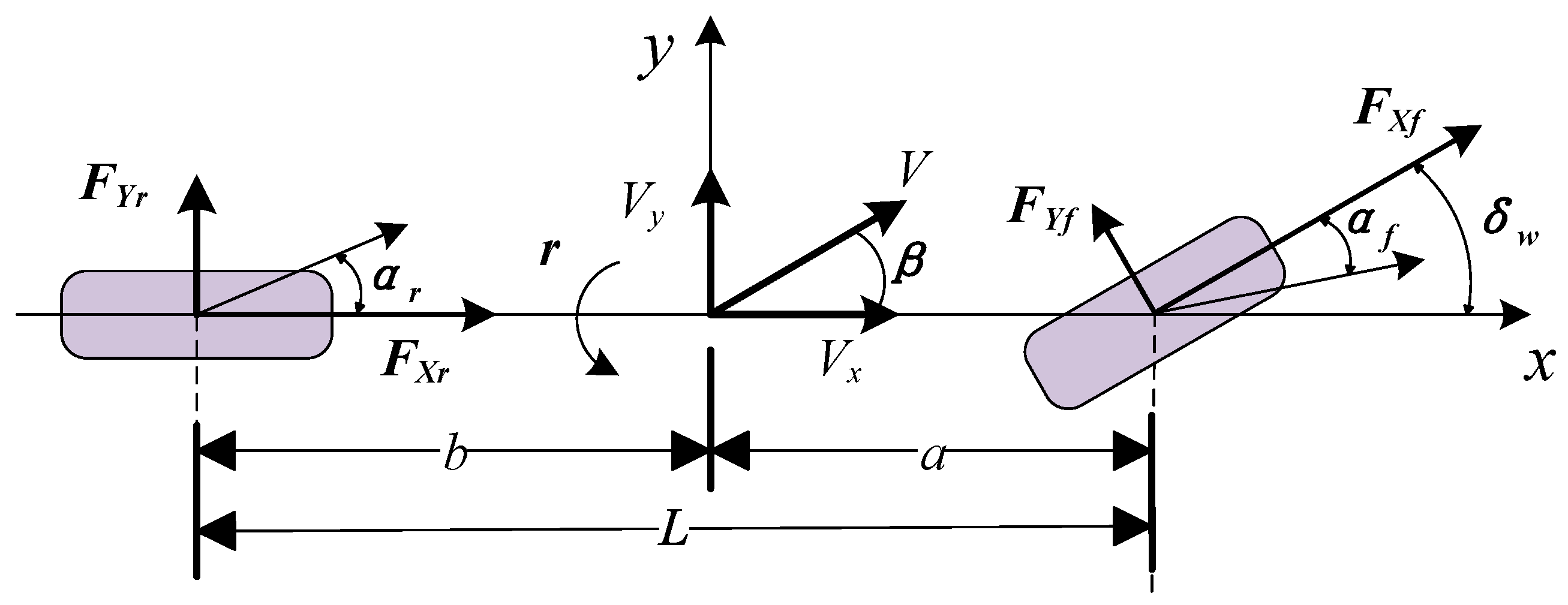
In the field of vehicle dynamics, in order to describe the vehicle yaw stability, it is usually simplified to a two-degree-of-freedom model (2-DOF). This model can describe the lateral and yaw motion of the vehicle. The reference values of the yaw rate and side slip angle required for stability control can be directly calculated using the two-degree-of-freedom vehicle model, as shown in Figure 2.

As a complex system, the vehicle model needs to be simplified in order to facilitate the study of vehicle yaw stability. The vehicle two-degree-of-freedom model is a commonly used dynamic model to study vehicle yaw stability, but a series of assumptions are required in the process of introducing the vehicle two-degree-of-freedom model:

(1)

Ignore the steering system and directly control the front wheel angle.

(2)

Ignore the suspension and think that the vehicle only moves parallel to the ground.

(3)

Ignore the effect of air resistance.

(4)

Ignore the relationship between tire longitudinal and lateral forces.

(5)

Neglect changes in wheel characteristics caused by vertical load fluctuations.

(6)

Ignore the tire backing torque.

(7)

Since the tire lateral acceleration is small, the tire cornering force is within the linear range.

(8)

The vehicle’s speed $V_x$ is a fixed value.

According to Newton’s second law, the two-degree-of-freedom dynamics model of the vehicle can be obtained.

$$m{a}_y=F_{Yf}\cos {\delta }_w+F_{Yr}$$

(1)

$$I_z{\dot{\omega }}_r=a{F}_{Yf}\cos {\delta }_w-b{F}_{Yr}$$

(2)

$$a_y=v_x\dot{\beta }+v_x{\omega }_r$$

(3)

$$F_{Yf}=K_f{a}_f$$

(4)

$$F_{Yr}=K_r{a}_r$$

(5)

Assuming that the vehicle speed $V_x$ remains constant and the front wheel steering angle is small, the following approximation can be made:

$$\cos {\delta }_w\approx 1$$

(6)

$$a_f\approx {\delta }_w-\beta -\frac{a{\omega }_r}{V_x}$$

(7)

$$a_r\approx \frac{b{\omega }_r}{V_x}-\beta$$

(8)

Substituting Formulas (1)–(6) into Formulas (7) and (8), we can obtain:

$$\left\{\begin{array}{c}\dot{\beta }=-\frac{K_f+K_r}{m{V}_x}\beta +(\frac{a{K}_f-b{K}_r}{m{V}_x{}^2}-1){\omega }_r+\frac{K_f}{m{V}_x}{\delta }_w\\ {\dot{\omega }}_r=\frac{b{K}_r-a{K}_f}{I_z}\beta -\frac{a^2{K}_f+b^2{K}_r}{I_z{V}_x}{\omega }_r+\frac{a{K}_f}{I_z}{\delta }_w\hfill \end{array}\right.$$

(9)

In the formula, $m$ is the sprung mass of the vehicle; F_Yf is the lateral force on the ground received by the tires of the front axle of the vehicle; F_Yr is the lateral force on the ground received by the tires of the front axle of the vehicle; ${\delta }_w$ is the front wheel steering angle; $I_z$ is the vehicle’s moment of inertia around the z-axis; ${\omega }_r$ is the yaw rate; a is the distance from the front axle to the center of mass; b is the distance from the rear axle to the center of mass; K_f and K_r are the cornering stiffness of the front and rear axle tires, respectively; α_f and α_r are the side slip angles of the front and rear axle tires, respectively; V_x is the longitudinal speed of the vehicle; β is the side slip angle.

From Equation (9), the general form of the state space equation can be derived:

$$\dot{X}=AX+B{\delta }_w$$

(10)

where $X={\left[\begin{array}{cc}\beta & {\omega }_r\end{array}\right]}^T$.

The expression of matrix A is

$$A=\left[\begin{array}{cc}-\frac{K_f+K_r}{mVx}& \frac{b{K}_r-a{K}_f}{mV{x}^2}-1\\ \frac{b{K}_r-a{K}_f}{I_z}& \frac{a{K}_f+b^2{K}_r}{I_z{V}_x}\end{array}\right]$$

(11)

The expression of matrix B is

$$B={\left[\begin{array}{cc}\frac{K_f}{m{V}_x}& \frac{a{K}_f}{I_z}\end{array}\right]}^T$$

(12)

2.2. Yaw Stability Control Target

There are two main reasons for the yaw instability of the vehicle during high-speed driving: (1) the yaw rate cannot follow the reference value, which makes the vehicle unstable, and (2) the deviation of the side slip angle cannot always return to zero, which results in the continuous accumulation of deviations in the vehicle’s driving path, and eventually makes it unstable. Therefore, the side slip angle and yaw rate are the preferred control targets of most of the yaw stability control strategies.

The reference value of the yaw rate can be calculated through the two-degree-of-freedom model, and its expression is

$${\omega }_d=\frac{V_x}{L(1+K{V}_x{}^2)}{\delta }_w$$

(13)

In the formula, δ_w is the front wheel angle; L is the wheelbase; K is the stability factor, which is an important parameter to characterize the steady-state response of the vehicle, and its value is

$$K=\frac{m}{L^2}(\frac{a}{K_r}-\frac{b}{K_f})$$

(14)

Usually, the driver does not want the vehicle to deviate from the desired path, so the smaller the side slip angle, the better. In this paper, the target value of the side slip angle is set to 0.

2.3. Yaw Stability Control Based on Linear Quadratic Programming

When the vehicle is running at high speed, it is easily affected by external disturbances, and a deviation between the actual value and the reference value of the side slip angle and yaw rate will inevitably occur. In this case, the deviation can be adjusted by applying an additional yaw moment to the vehicle in order to follow the target value and ensure high stability.

In the early stage, even when the vehicle state parameters deviate, they can still be considered a linear system. If a yaw moment is applied to the car at this time, its dynamic equation is given by

$$\left\{\begin{array}{c}\dot{\beta }=-\frac{K_f+K_r}{m{V}_x}\beta +(\frac{a{K}_f-b{K}_r}{m{V}_x{}^2}-1){\omega }_r+\frac{K_f}{m{V}_x}{\delta }_w\\ {\dot{\omega }}_r=\frac{b{K}_r-a{K}_f}{I_z}\beta -\frac{a^2{K}_f+b^2{K}_r}{I_z{V}_x}{\omega }_r+\frac{a{K}_f}{I_z}{\delta }_w+\frac{\Delta M}{I_z}\end{array}\right.$$

(15)

Expressed in the form of state-space equations:

$$\dot{X}=AX+B{\delta }_w+D\Delta M$$

(16)

where $D={\left[\begin{array}{cc}0& \frac{1}{I_z}\end{array}\right]}^T$, ∆M-additional yaw moment.

Subtract Formula (10) from Formula (16) to obtain

$$\Delta \dot{X}=A\Delta X+D\Delta M$$

(17)

where $\Delta X={\left[\begin{array}{cc}\Delta \beta & \Delta {\omega }_r\end{array}\right]}^T$.

Written in general form:

$$\dot{x}=Ax+Du$$

(18)

where $x=\Delta X$ is the state quantity, $u=\Delta M$ is the control amount.

Equation (18) describes the dynamic relationship between the additional yaw moment and the error of the vehicle stability parameters. Based on this relationship, the required additional yaw moment can be calculated using the linear quadratic programming (LQR) method.

When using the LQR method, it is crucial to establish a cost function. This paper uses the cost function expressed in Equation (19) to evaluate the relationship between the vehicle motion state and the additional yaw moment. This cost function can perform the real-time adjustment of the control quantity and make the optimal decision of the additional yaw moment at all times.

$$J=\frac{1}{2}{\displaystyle {\int }_0^{\infty }(x^{T}Qx+u^{T}Ru)}dt$$

(19)

On the one hand, the input deviation should be small (i.e., x should be as small as possible). On the other hand, it is hoped that the paid price will be relatively small (i.e., u should be as small as possible). This cost function reflects the controller’s requirements on the state error and on the additional yaw moment.

A feedback controller is then designed according to the control method of LQR.

$$u_{def}=-Kx$$

(20)

The feedback coefficient is $K=R^{-1}{B}^{T}P$.

P can be obtained by solving the following Riccati equation

$$A^{T}P+PA+Q+K^{T}RK-K^T{B}^{T}P-PBK=0$$

(21)

The weight coefficient matrices Q and R are crucial for the optimization of the linear quadratic matrix. Since the linear change of the evaluation index does not significantly affect the control rate, R can be considered equal to 1. Compared with the weight coefficient matrix R, it is more necessary to focus on adjusting Q. Considering the actual physical meaning of the vehicle stability control, the Q matrix is written in diagonal form as

$$Q=\left[\begin{array}{cc}{q}_1& 0\\ 0& q_2\end{array}\right]$$

(22)

Then, the cost function can be written as

$$J=\frac{1}{2}{\displaystyle {\int }_0^{\infty }[q_{{}_1}\cdot \Delta {\beta }^2(t)+q_{{}_{{}^2}}\cdot \Delta r^2(t)+\Delta M^2(t)]}dt$$

(23)

Among them, $q_1$ reflects the degree to which the cost function attaches importance to the side slip angle error, and $q_2$ reflects the degree to which the cost function attaches importance to the yaw rate error. The values of $q_1$ and $q_2$ can be flexibly set according to different working conditions.

After calculating the value of K, substituting K into Formula (18) can obtain the optimal additional yaw moment $\Delta M$.

$$\Delta M=u_{def}=-Kx=-k_1\Delta \beta -k_2\Delta \omega$$

(24)

2.4. Additional Yaw Moment Distribution Strategy

The total braking torque Tb is linearly related to the depth of the brake pedal. Based on the total braking torque, a torque difference is generated between the four motors, which forms an additional yaw moment $\Delta M$. Therefore, the braking torque allocated to each motor should meet the following conditions.

$$\left\{\begin{array}{l}{T}_{rl}+T_{rr}+T_{fl}+T_{fr}=T_b\hfill \\ \frac{(T_{fr}+T_{rr}-T_{rl}-T_{fl})\frac{w}{2}}{r}=\Delta M\hfill \end{array}\right.$$

(25)

In the formula, T_fl, T_fr, T_rl, T_rr represent the torque of the four wheels of the vehicle, respectively, and w is the wheelbase.

From this, we can obtain the torque distribution of four-wheel braking as

$$\left\{\begin{array}{c}{T}_{fl}=\frac{T_b}{4}-\frac{\Delta Mr}{2w}\\ \begin{array}{l}{T}_{fr}=\frac{T_b}{4}+\frac{\Delta Mr}{2w}\\ T_{rl}=\frac{T_b}{4}-\frac{\Delta Mr}{2w}\\ T_{rr}=\frac{T_b}{4}+\frac{\Delta Mr}{2w}\end{array}\end{array}\right.$$

(26)

3. Roll Stability Control

3.1. Three Degrees of Freedom Model of Vehicle Roll

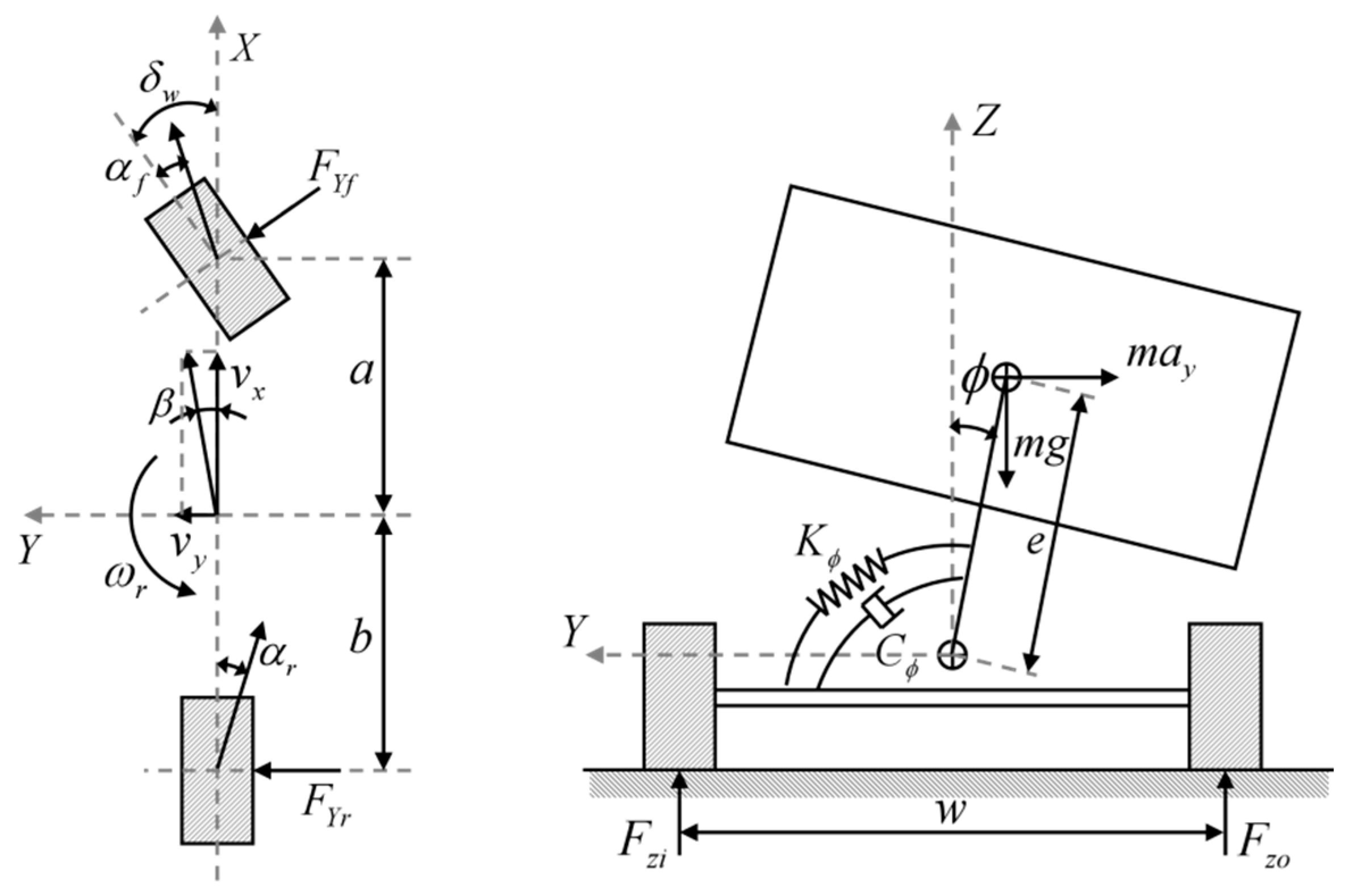
In order to monitor the roll state of the vehicle, it is necessary to introduce a three-degree-of-freedom model of the vehicle, as shown in Figure 3. This model not only considers the two degrees of freedom of lateral and yaw but also considers the degree of freedom of roll.

The dynamics equation of the vehicle is

$$m{a}_y-me\ddot{\varphi }=F_{Yf}\cos {\delta }_w+F_{Yf}$$

(27)

$$I_z{\dot{\omega }}_r=a{F}_{Yf}\cos {\delta }_w-b{F}_{Yr}$$

(28)

$$I_x\ddot{\varphi }+C_{\varphi }\dot{\varphi }+K_{\varphi }\varphi =mge\sin \varphi +m{a}_{y}e\cos \varphi$$

(29)

$$a_y=v_x\dot{\beta }+v_x{\omega }_r$$

(30)

$$F_{Yf}=K_f{\alpha }_f$$

(31)

$$F_{Yr}=K_r{\alpha }_r$$

(32)

When the vehicle speed V_x is constant and the front wheels are in a state of small steering angle, the following approximation can be made:

$$\left\{\begin{array}{c}\cos \delta w\approx 1\\ \cos \varphi \approx 1\\ \sin \varphi \approx \varphi \end{array}\right.$$

(33)

$${\alpha }_f\approx {\delta }_w-\beta -\frac{a{\omega }_r}{V_x}$$

(34)

$${\alpha }_r\approx \frac{b{\omega }_r}{V_x}-\beta$$

(35)

$$\beta \approx \tan \beta =\frac{V_y}{V_x}$$

(36)

Arranged into the state equation, we can obtain

$$\dot{X}=AX+B{\delta }_w$$

(37)

state variable $X={\left[\begin{array}{cccc}\beta & {\omega }_r& \dot{\varphi }& \varphi \end{array}\right]}^T$.

Matrix A is

$$A=\left[\begin{array}{cccc}-\frac{(K_f+K_r)I_x}{m{V}_x(I_x-m{e}^2)}& \frac{I_x}{m(I_x-m{e}^2)}(\frac{b{K}_r-a{K}_f}{m{V}_x{}^2}-1)& -\frac{e{C}_{\varphi }}{V_x(I_x-m{e}^2)}& -\frac{mg{e}^2-e{K}_{\varphi }}{V_x(I_x-m{e}^2)}\\ \frac{b{K}_r-a{K}_f}{I_z}& -\frac{a^2{K}_f+b^2{K}_r}{I_z{V}_x}& 0& 0\\ -\frac{(K_f+K_r)e}{I_x-m{e}^2}& \frac{(K_{r}b-K_{f}a)e}{(I_x-m{e}^2)V_x}& -\frac{C_{\varphi }}{I_x-m{e}^2}& -\frac{mge-K_{\varphi }}{I_x-m{e}^2}\\ 0& 0& 1& 0\end{array}\right]$$

(38)

Matrix B is

$$B={\left[\begin{array}{cccc}\frac{K_f{I}_x}{m{V}_x(I_x-m{e}^2)}& \frac{a{K}_f}{I_z}& \frac{K_{f}e}{I_x-m{e}^2}& 0\end{array}\right]}^T$$

(39)

Among them, m is the sprung weight of the vehicle; F_Yf is the ground lateral force on the front axle tire; F_Yr is the ground lateral force on the rear axle tire; δ_w is the front wheel steering angle; a_y is the lateral acceleration; $\varnothing$ is the roll angle; e is the distance from the roll center to the center of mass of the vehicle; $K_{\varnothing }$ is the roll stiffness of the vehicle body; $C_{\varnothing }$ is the roll damping coefficient; I_Z is the moment of inertia of the vehicle around the z-axis; β is the side slip angle; ω_r is the yaw rate; a is the distance from the front axle to the center of mass; b is the distance from the rear axle to the center of mass; α_f, α_r are the side slip angles of the front and rear axle tires, respectively; K_f and K_r are the roll stiffnesses of the front and rear axle tires, respectively; V_x and V_y are, respectively, the longitudinal and lateral speeds of the vehicle.

3.2. Roll Stability Controller

Based on the dynamic equation obtained from the three-degree-of-freedom model of the vehicle, an additional yaw moment can be added to the yaw dynamic equation around the Z axis to obtain the dynamic equation:

$$\left\{\begin{array}{c}m{a}_y-me\ddot{\varphi }=F_{Yf}\cos {\delta }_w+F_{Yr}\\ I_z{\dot{\omega }}_r=a{F}_{Yf}\cos {\delta }_w-b{F}_{Yr}+\Delta M_d\\ I_x\ddot{\varphi }+C_{\varphi }\dot{\varphi }+K_{\varphi }\varphi =mge\sin \varphi +m{a}_{y}e\cos \varphi \end{array}\right.$$

(40)

Rearranging Formula (40) can obtain the following state space equation:

$$\begin{array}{c}\dot{X}(t)=AX(t)+Bu(t)+B_{1}d(t)\\ y(t)=CX(t)\end{array}$$

(41)

where the A matrix is

$$A=\left[\begin{array}{cccc}-\frac{(K_f+K_r)I_x}{m{V}_x(I_x-m{e}^2)}& \frac{I_x}{m(I_x-m{e}^2)}(\frac{b{K}_r-a{K}_f}{m{V}_x{}^2}-1)& -\frac{e{C}_{\varphi }}{V_x(I_x-m{e}^2)}& -\frac{mg{e}^2-e{K}_{\varphi }}{V_x(I_x-m{e}^2)}\\ \frac{b{K}_r-a{K}_f}{I_z}& -\frac{a^2{K}_f+b^2{K}_r}{I_z{V}_x}& 0& 0\\ -\frac{(K_f+K_r)e}{I_x-m{e}^2}& \frac{(K_{r}b-K_{f}a)e}{(I_x-m{e}^2)V_x}& -\frac{C_{\varphi }}{I_x-m{e}^2}& -\frac{mge-K_{\varphi }}{I_x-m{e}^2}\\ 0& 0& 1& 0\end{array}\right]$$

(42)

where the B matrix is

$$B={\left[\begin{array}{cccc}0& \frac{1}{I_z}& 0& 0\end{array}\right]}^T$$

(43)

where the B₁ matrix is

$$B_1={\left[\begin{array}{cccc}\frac{K_f{I}_x}{m{V}_x(I_x-m{e}^2)}& \frac{a{K}_f}{I_z}& \frac{K_{f}e}{I_x-m{e}^2}& 0\end{array}\right]}^T$$

(44)

where the C matrix is

$$C=\left[\begin{array}{cccc}0& 0& 1& 0\end{array}\right]$$

(45)

The input of the entire control system is the additional yaw moment $∆M_d$, the output of the system is the roll angle of the center of mass of the vehicle Φ, and the front wheel rotation angle δ_w is used as the disturbance input item. The state quantity of this controller is $X\left(t\right)={\left[\beta {\omega }_r \dot{\varnothing } \varnothing \right]}^T$, the input quantity $u\left(t\right)=∆M_d$, the output $y\left(t\right)=\varnothing$, and the disturbance input $d\left(t\right)={\delta }_w$.

Before applying the model predictive control theory, Formula (41) needs to be discretized, and the forward Euler method should be used for discretization.

$$\dot{X}(t)=\frac{X(t+1)-X(t)}{\Delta t}=AX(t)+Bu(t)+B_1\mathrm{d}\left(\mathrm{t}\right)$$

(46)

Rearranged to

$$X(t+1)=(I+A)\Delta tX(t)+B\Delta tu(t)+B_1\Delta td(t)$$

(47)

make

$$F=(I+A)\Delta t$$

(48)

$$B_u=B\Delta t$$

(49)

$$B_d=B_1\Delta t$$

(50)

Then, the original Formula (47) can be written as

$$X(t+1)=FX(t)+B_{u}u(t)+B_{d}d(t)$$

(51)

Equation (51) is the discrete state equation. Based on the current state of the vehicle system at time k, the state of the vehicle in the future p steps is predicted. At this time, the system prediction time domain is p, and the control time domain is m (m < p). At the same time, the following assumptions need to be made:

(1)

Assume that the control quantity does not change after controlling the time domain m.

(2)

Assume that the disturbance input does not change after time k.

The system state quantity returned by the vehicle sensor at time k is x(k) (including n state quantities), which is used as the starting point of prediction to predict the system state at time k + 1, k + 2…k + p in the future.

Recursively deduce the discrete state equation, and we can obtain

$$\begin{array}{cc}\hfill x(k\left|k\right.)& =x(k)\hfill \\ \hfill x(k+1\left|k\right.)& =Fx(k\left|k\right.)+B_{u}u(k)+B_{d}d(k)\hfill \\ \hfill x(k+2\left|k\right.)& =Fx(k+1\left|k\right.)+B_{u}u(k+1)+B_{d}d(k+1)\hfill \\ & =F^{2}x(k)+F{B}_{u}u(k)+F{B}_{d}d(k)+B_{u}u(k+1)+B_{d}d(k+1)\\ & ⋮\hfill \\ \hfill x(k+p\left|k\right.)& =F^{p}x(k)+F^{p-1}{B}_{u}u(k)+F^{p-1}{B}_{d}d(k)+F^{p-2}{B}_{u}u(k+1)\hfill \\ & +F^{p-2}{B}_{d}d(k+1)+\dots +B_{u}u(k+p-1)+B_{d}d(k+p-1)\hfill \end{array}$$

(52)

make

$$X_p={\left[\begin{array}{c}x(k\left|k\right.)\\ x(k+1\left|k)\right.\\ x(k+2\left|k)\right.\\ \begin{array}{c}⋮\\ x(k+p\left|k)\right.\end{array}\end{array}\right]}_{n(p+1)\times 1}$$

(53)

$$X(k)={\left[\begin{array}{c}x(k)\\ x(k)\\ ⋮\\ x(k)\end{array}\right]}_{n\times 1}$$

(54)

$$U(k)={\left[\begin{array}{c}u(k)\\ u(k+1)\\ u(k+2)\\ \begin{array}{c}⋮\\ u(k+m-1)\end{array}\end{array}\right]}_{m\times 1}$$

(55)

$$D(k)={\left[\begin{array}{c}d(k)\\ d(k+1)\\ d(k+2)\\ \begin{array}{c}⋮\\ d(k+m-1)\end{array}\end{array}\right]}_{m\times 1}$$

(56)

Organized to obtained X_p = MX(k) + LU(k) + ND(k)

where

$$M={\left[\begin{array}{c}I\\ F\\ F^2\\ \begin{array}{c}⋮\\ F^p\end{array}\end{array}\right]}_{n(p+1)\times n}$$

(57)

$$L={\left[\begin{array}{cccc}0& 0& & 0\\ B_u& 0& \cdots & 0\\ F{B}_u& B_u& & 0\\ \begin{array}{c}⋮\\ F^{p-1}{B}_u\end{array}& \begin{array}{c}⋮\\ F^{p-2}{B}_u\end{array}& \begin{array}{c}\ddots \\ \cdots \end{array}& \begin{array}{c}⋮\\ B_u\end{array}\end{array}\right]}_{n(p+1)\times m}$$

(58)

$$N={\left[\begin{array}{cccc}0& 0& & 0\\ B_d& 0& \cdots & 0\\ F{B}_d& B_d& & 0\\ \begin{array}{c}\\ F^{p-1}{B}_d\end{array}& \begin{array}{c}⋮\\ F^{p-2}{B}_d\end{array}& \begin{array}{c}\ddots \\ \cdots \end{array}& \begin{array}{c}⋮\\ B_d\end{array}\end{array}\right]}_{n(p+1)\times m}$$

(59)

$$\begin{array}{l}Y={\left[\begin{array}{c}y(k\left|k\right.)\\ y(k+1\left|k\right.)\\ y(k+2\left|k\right.)\\ \begin{array}{c}⋮\\ y(k+p\left|k\right.)\end{array}\end{array}\right]}_{\left(\mathrm{p}+1\right)\times 1}=C{X}_p\\ =CMX(k)+CLU(k)+CND(k)\end{array}$$

(60)

3.3. Quadratic Programming Solution

The model predictive (MPC) algorithms require the design of a cost function according to the control objective. Equation (61) ensures the minimum error between the output and reference values while ensuring the minimum change of the control input. Based on these requirements, the discrete state equation can be transformed into a quadratic programming problem.

$$J(k)={(Y_p-R_e)}^T\overline{Q}(Y_p-R_e)+U{(k)}^T\overline{R}U(k)$$

(61)

In the formula, R_e is the reference value matrix input by the model predictive control, and the control target is the center of mass roll angle. Here, the reference value is set to 0; that is, R_e is a zero matrix.

In order to solve the quadratic optimization problem, the objective function J is transformed into the form of z^THz + 2fz. Substituting Formula (60) into Formula (61) and rearranging, we obtain

$$\begin{array}{l}J(k)={(Y_p-{\mathrm{R}}_e)}^T\overline{Q}(Y_p-{\mathrm{R}}_e)+U{(k)}^T\overline{R}U(k)\\ =U{(k)}^T(L^T{C}^T\overline{Q}LC+\overline{R})U(k)\\ +2(X{(k)}^T{M}^T{C}^T\overline{Q}CL+D{(k)}^T{N}^T{C}^T\overline{Q}CL)U(k)+\dots \end{array}$$

(62)

It can be seen from the comparison that z = U(k), $H=L^T{C}^{T}QCL+\overline{R}$,

$${f=2(X\left(k\right)}^T{M}^T{C}^{T}QCL+{D\left(k\right)}^T{N}^T{C}^{T}QCL)$$

Since the changes in the remaining items do not affect the optimization of U(k), they can be ignored.

3.4. Wheel Torque Distribution

When a high-speed vehicle is in a turning condition, due to the axle load transfer, its tendency to dump to the outside will increase the vertical load of the outer wheel, and the upper limit of its braking force will also increase accordingly. Therefore, to weaken the vehicle’s tendency to roll over, this study uses the outer front wheel braking method. The force analysis of the outer front wheel shows that

$$\frac{T_b}{r}\cdot a\cdot \sin {\delta }_w+\frac{T_b}{r}\cdot \frac{w}{2}\cdot \cos {\delta }_w=\Delta M_d$$

(63)

The braking torque of the outer front wheel can be obtained by sorting out

$$T_b=\frac{\Delta M_{d}r}{a\sin {\delta }_w+\frac{w}{2}\cos {\delta }_w}$$

(64)

3.5. Coordination Strategy of Yaw Stability Control and Roll Stability Control

At present, the lateral load transfer ratio (LTR) is a widely used rollover indicator. The lateral load transfer rate can express the change in the vertical load of the vehicle, and its expression is

$$LTR=\frac{F_{zl}-F_{zr}}{F_{zl}+F_{zr}}$$

(65)

In the formula, F_zl is the vertical load of the left tire of the vehicle, and F_zr is the vertical load of the right tire.

When the vehicle rolls over to a certain side or before the rollover, its vertical load will continue to decrease; that is, the wheels will gradually lift off the ground. When the vertical load of a wheel on a certain side is 0, it is considered that a rollover has occurred. That is, when F_zl = 0 or F_zr = 0, LTR = 1 is equivalent to the rollover of the vehicle. The value range of LTR is [–1, 1].

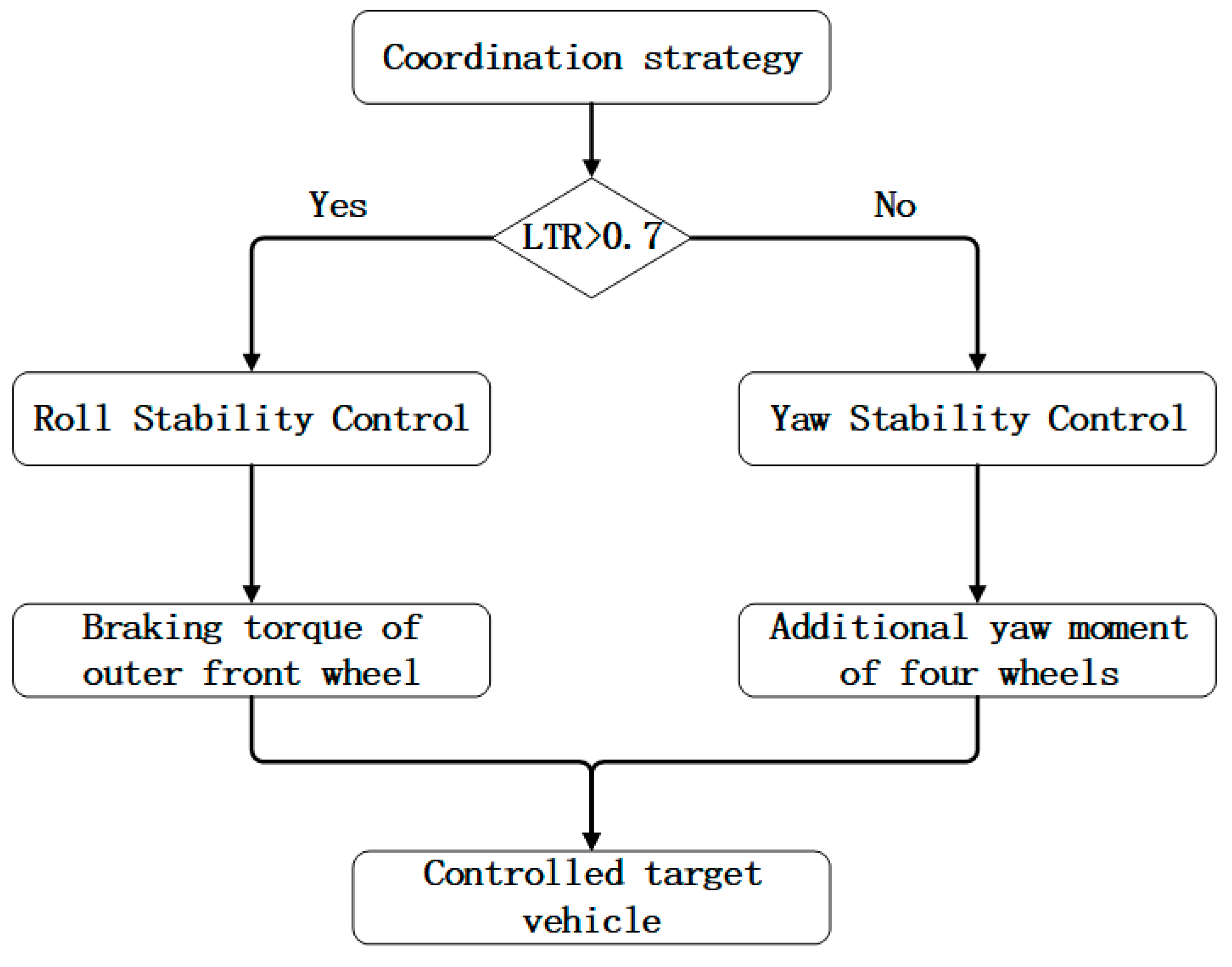
Large commercial vehicles, such as city buses, are prone to roll instability due to their high center of mass. Once the vehicle rolls over, it will directly threaten the life and safety of the driver and passengers. Therefore, the roll stability should be given priority over the yaw stability. When the vehicle is running normally, the yaw stability controller guarantees its stability. When the roll judgment index gradually increases and reaches the threshold, the vehicle roll stability controller starts to intervene, initializes the four-wheel torque to be evenly distributed, and adds roll yaw moment on this basis. As shown in Figure 4.

4. Simulation Result Analysis

4.1. Co-Simulation Platform

This study builds a MATLAB/Simulink 2021b and Trucksim 2020 joint simulation platform. The stability control algorithm of the vehicle is implemented in MATLAB/Simulink, and the control strategy is used to control the simulated vehicle of Trucksim using the co-simulation platform in order to verify the effectiveness of the proposed control strategy.

The vehicle parameters are shown in

Table 1. Vehicle parameters.

Parameter	Value	Parameter	Value
Vehicle mass (kg)	11,600	Body roll damping (Nms/rad)	38,000
Wheelbase (m)	6.15	Roll stiffness of front axle tires (N/rad)	110,000
Distance from front axle to center of mass (m)	3.85	Roll stiffness of rear axle tires (N/rad)	200,000
Distance from rear axle to center of mass (m)	2.3	Moment of inertia of X axis (kg m2)	17,036.8
Distance between left and right wheel tires (m)	1.903	Moment of inertia of Z axis (kg m2)	71,058
Vehicle centroid height (m)	1.5	Rolling radius of the tire (m)	0.465
Body roll stiffness (Nm/rad)	500,000

.

4.2. Simulation Verification of Yaw Stability

In order to verify the effectiveness of the stability control algorithm under braking conditions, two conditions are designed:

(1)

Steering wheel angle step condition;

(2)

Serpentine condition.

When the vehicle has yaw instability, it is usually accompanied by deviation, and thus, the road surface adhesion coefficient should not have a high value. Otherwise, the vehicle will roll over, which does not meet the verification conditions for yaw stability. The road surface adhesion coefficient is set to 0.3 in Trucksim. The simulation conditions are shown in

Table 2. Parameters of simulation working conditions.

Condition Name	Braking Force	Initial Speed	Steering Wheel Angle	Road Surface Adhesion Coefficient
Steering wheel angle step condition	5000 N	90	60	0.3
Serpentine condition	5000 N	90	90	0.3

.

4.2.1. Steering Wheel Angle Step Input

The steering wheel angle step input is shown in Figure 5.

The simulation results are shown in Figure 6.

It can be seen from Figure 6b,c that the yaw rate and the side slip angle have good control effects. The actual yaw rate can accurately follow the target value. The side slip angle is also stable near the target value of 0, with an amplitude range of [0, 0.081], and it steadily decreases under the action of the control algorithm. The simulation results without control are shown in Figure 6d,e. The yaw rate sharply increases, and the vehicle trajectory significantly deviates. The side slip angle also reaches a large magnitude in the range of (−3.14, 3.13). During the entire simulation process, the stability control algorithm reduces the maximum value of the side slip angle of the vehicle by 98.7%, which allows for effective avoidance of vehicle instability.

4.2.2. Serpentine Condition

The steering wheel input is shown in Figure 7.

The simulation results are shown in Figure 8.

The steering wheel input is sinusoidal with a maximum angle of 90° and two cycles in total, as shown in Figure 7. The following situation of the control target can be deduced from Figure 8b,c. The yaw rate can still follow the target value with high precision. In addition, the side slip angle can regularly change according to the changing trend of the steering wheel angle curve in the serpentine condition, which shows that the side slip angle is also controlled. Figure 8d,e show that the vehicle without the stability control algorithm obviously loses control, and the sideslip situation is serious. Moreover, the yaw rate sharply increases. By comparing the specific data in Figure 8c,e, it can be deduced that the amplitude range of the side slip angle of the vehicle without adding the stability control algorithm is [−0.12, 0.12]. The amplitude range of the side slip angle of the vehicle added to the stability control algorithm is [−3.14, 3.14]. Throughout the simulation, the stability control algorithm reduces the vehicle’s side slip angle magnitude by 96.2%. In addition, according to the changing trend of the steering wheel angle, the side slip angle does not change. This shows that the vehicle is already in an unstable state at this time, and there is a phenomenon of flicking and turning around. The above conclusion can also be verified from the vehicle trajectory in Figure 8f. Under the action of the control algorithm, the driving route of the vehicle maintains a serpentine shape. The vehicle’s trajectory without the action of the stability control algorithm produces a large deviation and cannot maintain the serpentine condition.

4.3. Verification of Roll Stability

The fishhook condition is often used to evaluate the roll stability of the vehicle due to the fact that it can simulate the emergency avoidance situation that is prone to vehicle rollover. Therefore, this paper also adopts the fishhook working condition to verify the effectiveness of the proposed roll stability control algorithm.

Because the angle of the steering wheel significantly changes in the fishhook condition, the vehicle is more prone to rollover on roads with a high adhesion coefficient. Therefore, in order to verify the control effect of the roll stability algorithm, this paper considers this working condition for testing. In the simulation test, the initial vehicle speed and the road surface adhesion coefficient are set to 70 km/h and 0.85, respectively.

The simulation results of the fishhook conditions are shown in Figure 9.

It can be seen from Figure 9a that the steering wheel quickly turns left to the 90° position in 1 s and then maintains it for 0.25 s. Afterward, the steering wheel quickly turns to the right to the −90° position and then slowly returns to the initial position after holding for 3 s. The steering wheel is held for 2 s after returning to its original position. During the whole process, the steering wheel has a maximum rotation angle of 90°. This working condition can simulate the situation of emergency obstacle avoidance. It can be seen from Figure 9b that under the action of no stability control algorithm, the calculation of the LTR of the vehicle has stopped in more than 5 s, which indicates that it has completely rolled over at this time. However, the LTR value of the vehicle under the action of the stability control algorithm can return to normal, which proves that the roll control is effective. The roll angle and roll angular velocity are the indexes of the presented control quantification. It can be seen from Figure 9d,e that under the action of the stability control algorithm, the vehicle roll angle and the roll angular velocity can gradually return to a stable state when the LTR reaches 1. If the vehicle is not applied with stability control, its roll angle and roll rate sharply increase at 5 s, and finally, instability and rollover occur. It can be deduced from the specific data of the simulation that for 0–3 s, the intervention of the stability control algorithm has no significant influence on the roll angle curve of the vehicle. Within 3–6 s, the maximum roll angle of the vehicle without the stability control algorithm reaches 34.03°, while that with the stability control algorithm is only 6.44°. By comparing the specific data in Figure 9d, it can be deduced that the stability control algorithm can reduce the maximum value of the roll angle by 81.1% within 3–6 s. In addition, within 3–6 s, the maximum value of the vehicle’s roll rate without the stability control algorithm reaches 55.62 °/s, while that with the stability control algorithm is only 19.49 °/s. By comparing the specific data in Figure 9e, it can be seen that within 3–6 s, the stability control algorithm can reduce the maximum value of the roll angular velocity by 65.0%. It can also be seen from Figure 9f that under the action of the stability control algorithm, the vehicle’s lateral acceleration can gradually return to a steady state. Conversely, if no stability control is applied to the vehicle, its lateral acceleration will exhibit drastic changes until it eventually rolls over. By comparing the specific data in Figure 9f, it can be observed that the amplitude range of the lateral acceleration of the vehicle without adding the stability control algorithm is [−4.07, 5.38]. The amplitude range of the vehicle lateral acceleration added to the stability control algorithm is [−4.12, 4.28]. The stability control algorithm reduces the magnitude of the vehicle’s lateral acceleration by 11.1% throughout the simulation. Figure 9g shows that without the intervention of the stability control algorithm, the vehicle’s driving trajectory significantly deviates. Since the vehicle rolls over in the middle of driving, its driving distance is relatively short in the simulation. It can be seen from the simulation experiment of the fishhook condition that the roll stability control strategy has a good control effect.

5. Conclusions

In this paper, a vehicle yaw stability controller is designed based on the linear two-degree-of-freedom model and the LQR algorithm. A vehicle roll stability controller is also designed based on a linear three-degree-of-freedom model and an MPC algorithm. A coordinated control strategy for the yaw and roll stability is designed by considering the LTR as the condition of yaw and roll stability switching. In addition, the designed control strategy is verified by MATLAB/Simulink and Trucksim co-simulation.

5.1. Discussion and Analysis of Results

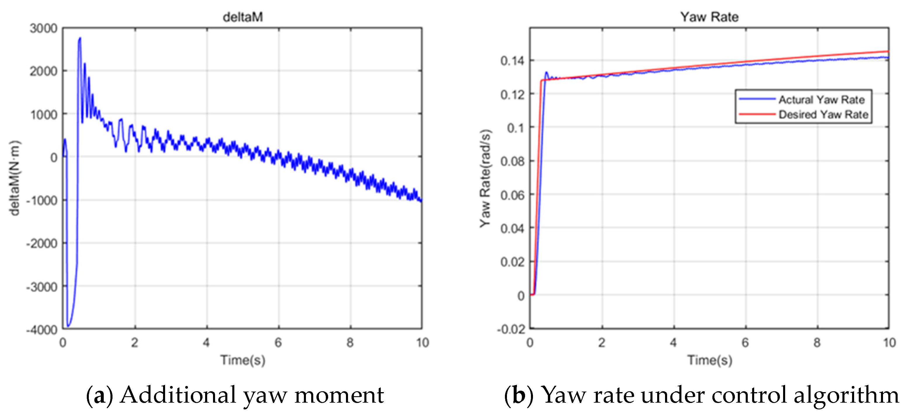
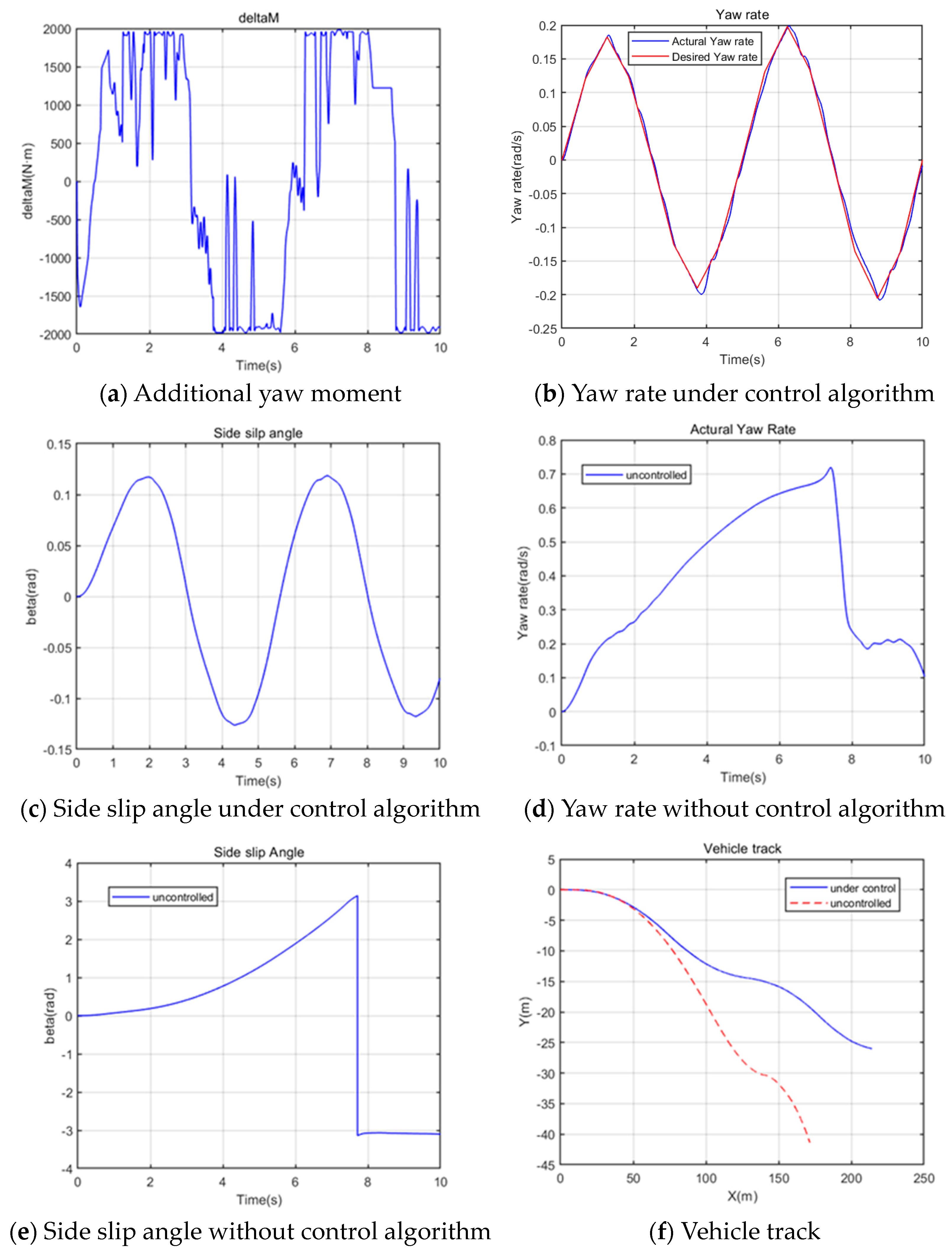
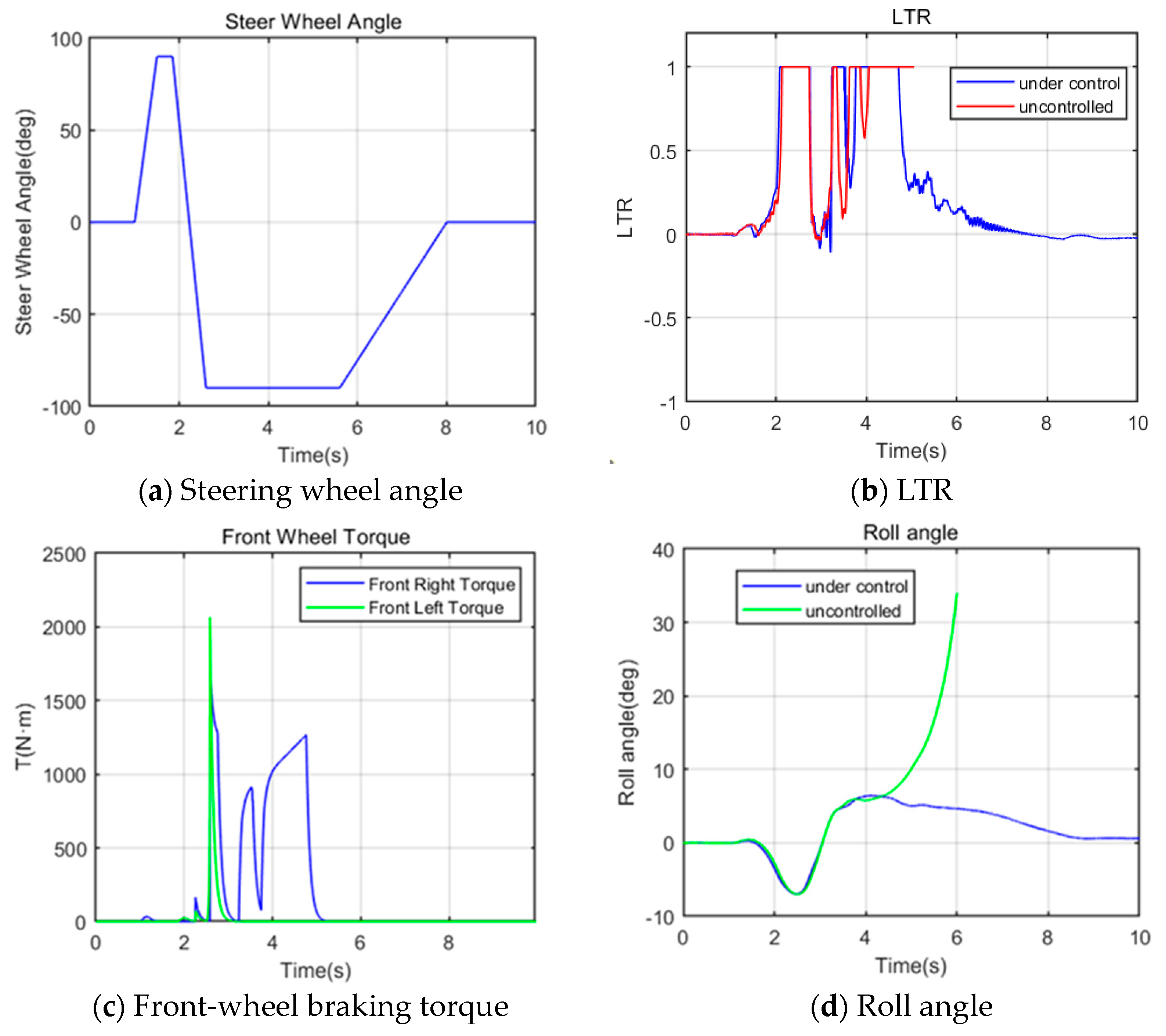
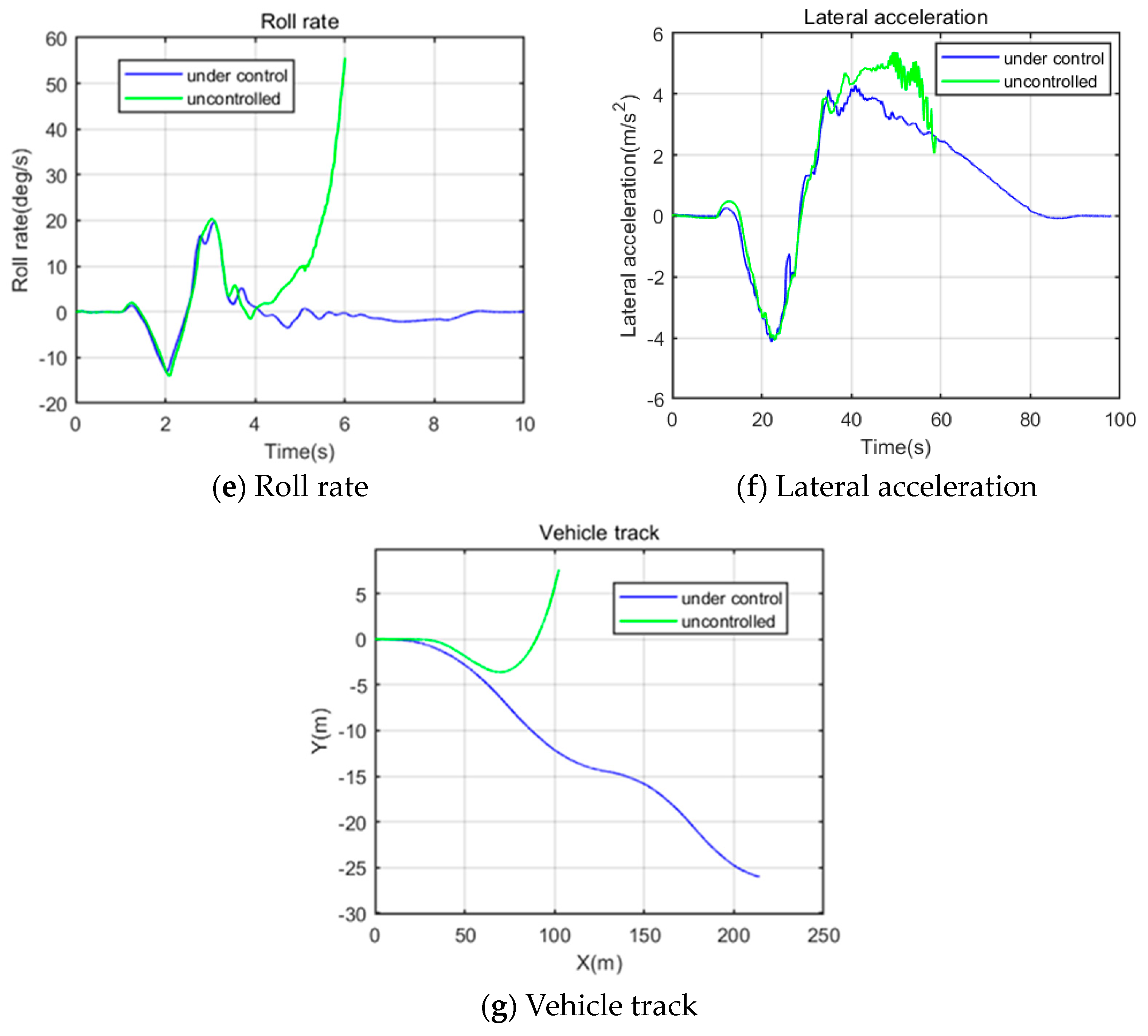
Compared with no control, in terms of yaw stability, the stability control algorithm can make the yaw rate track the target value with high precision, and it can also make the side slip angle regularly follow the real-time change of the steering wheel angle and reduce its amplitude size. As for the roll stability, the simulation results show that the stability control algorithm can significantly reduce the maximum magnitude of the curve responses of roll angle, roll angular velocity, and lateral acceleration, improve their respective convergence, and suppress the occurrence of rollover. From the simulation data results, when the vehicle is running at a high speed of 90 km/h, the stability control algorithm can control the yaw rate tracking error within 0.05 rad/s. In addition, the control algorithm can reduce the maximum amplitude of the side slip angle, the maximum value of the roll angle, the maximum value of the roll angular velocity, and the amplitude of the lateral acceleration by more than 96%, 81.1%, 65.0%, and 11.1%, respectively. It can be deduced from the analysis of the simulation results that the designed control algorithm has a good control effect in improving the electric bus’s yaw stability and roll stability.

The work in [37] is also based on distributed drive, a new electric vehicle drive architecture, and designs a stability coordination control algorithm that considers vehicle yaw and roll. However, [37] is different from this article in the specific selection of the control algorithm. The work in [37] uses the fuzzy control method for vehicle yaw and roll stability control. In terms of verifying the effectiveness of the control algorithm, working conditions similar to those in this article were used for simulation verification. Under the step input of the steering angle, the vehicle travels at 90 km/h. Under the control algorithm of [37], the maximum error of the actual yaw rate following the expected value reaches 0.03 rad/s. Under the control algorithm designed in this article, the maximum error of the actual yaw rate following the expected value is only within 0.01 rad/s. Under serpentine conditions, the vehicle travels at 90 km/h. Under the control algorithm of [37], the maximum error of the actual yaw rate following the expected value reaches 0.1 rad/s. Under the control algorithm designed in this article, the maximum error of the actual yaw rate following the expected value is only within 0.03 rad/s. Under the fishhook condition that easily causes the vehicle to roll, the vehicle travels at 70 km/h. Under the control algorithm of [37], the maximum roll angle reaches 0.02 rad, and the maximum roll angular speed reaches 0.04 rad/s. Under the control algorithm designed in this article, the maximum roll angle is only 0.0105 rad, and the maximum roll angle speed reaches 0.035 rad/s. This is due to the fact that the LQR control algorithm is superior to the fuzzy control algorithm in terms of control accuracy. Although the fuzzy control algorithm has the advantages of a simple control principle and no need to establish a clear mathematical model to achieve control, its control strategy relies heavily on experience design. The LQR algorithm is designed based on a two-degree-of-freedom model that can fully reflect the vehicle’s yaw properties, and an optimization objective function is designed to achieve the solution.

5.2. Future Research Prospects

It can be deduced from the analysis of the simulation results that the designed control algorithm has a good control effect in improving the electric bus’s yaw stability and roll stability.

However, room for improvement still exists. More precisely, the control algorithms can be further optimized. In addition, the control parameters in the LQR and MPC algorithms used in this paper are fixed. In future work, a variable parameter regulator or an adaptive algorithm can be introduced to meet the stability requirements of changing the working conditions. In terms of road surface conditions, this paper does not consider a model of aerodynamic-road surface interaction. In subsequent research, in order to further ensure the stability of the vehicle, the aerodynamic-road interaction model can be fully considered to guide the design of the control algorithm. Moreover, in terms of algorithm verification, no real vehicle test was conducted due to the danger of its conditions. Thus, the test conditions can be adjusted to verify the control effect of the control algorithm on the actual vehicle according to the requirements of the site and the safety of the test.