
Fuel-Efficiency Improvement by Component-Size Optimization in Hybrid Electric Vehicles


Abstract
1. Introduction
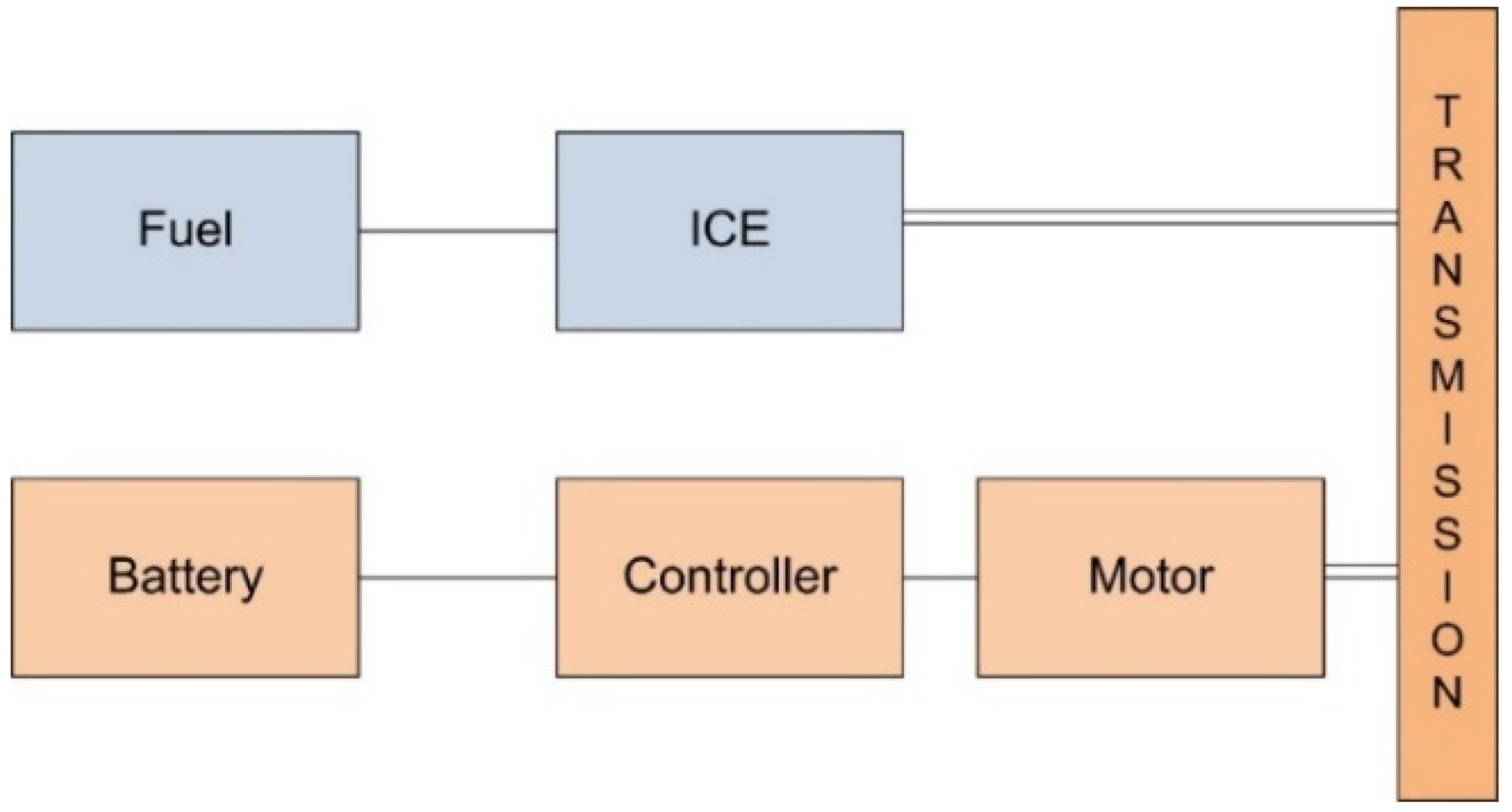
2. Modeling of Hybrid Electric Vehicles
2.1. ICE Modeling
2.1.1. Cranking
2.1.2. ICE off
2.1.3. Idle
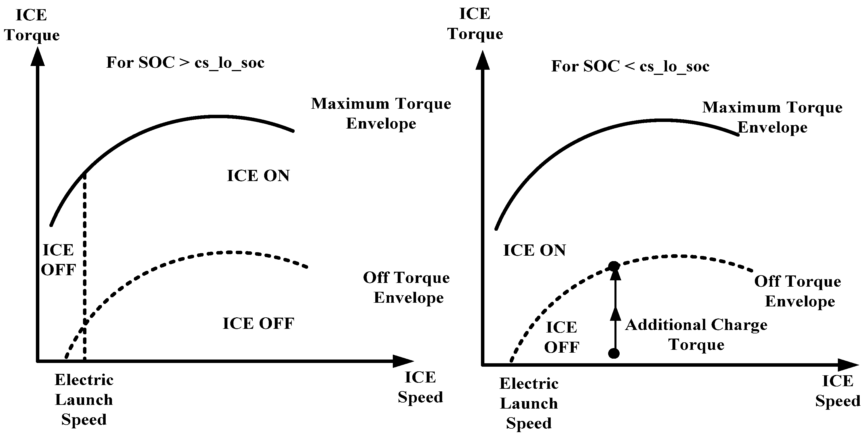
2.1.4. ICE on
2.2. Motor Modeling
2.2.1. Propulsion Mode
2.2.2. Regenerative Mode
2.2.3. Spinning Mode
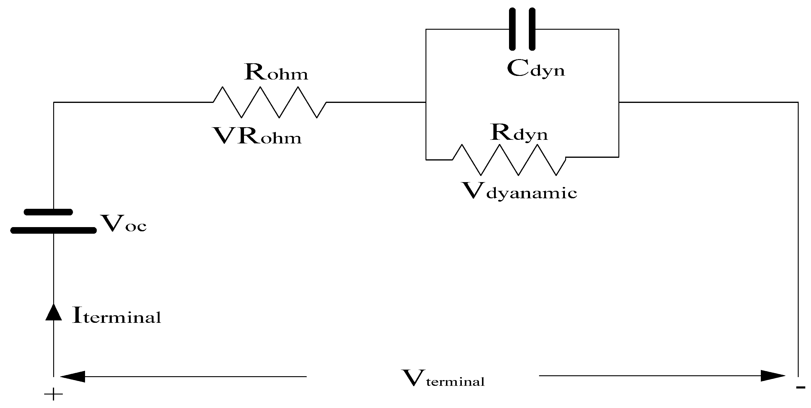
2.3. Battery Modeling
3. Problem Formulation
4. Energy Management System
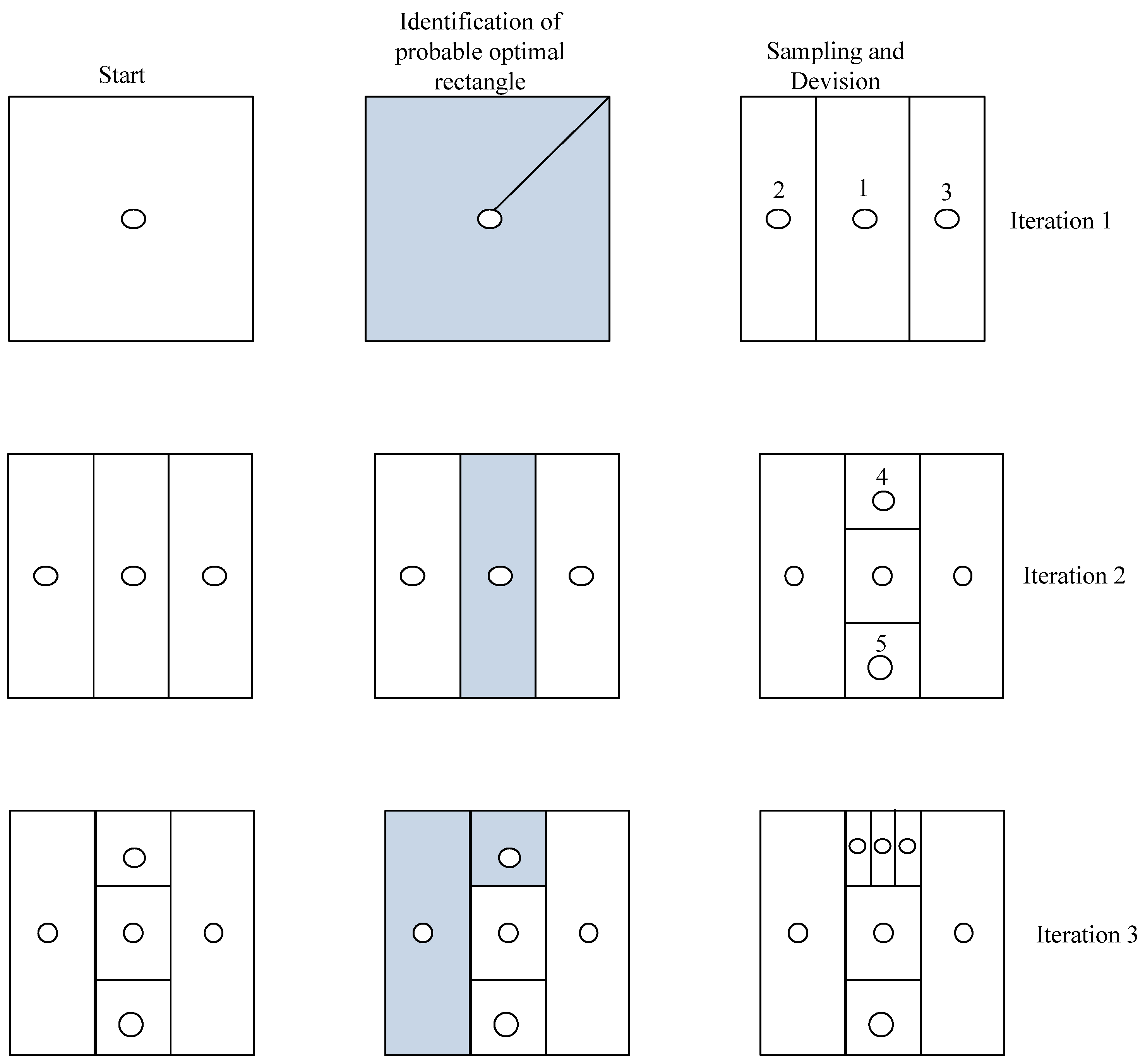
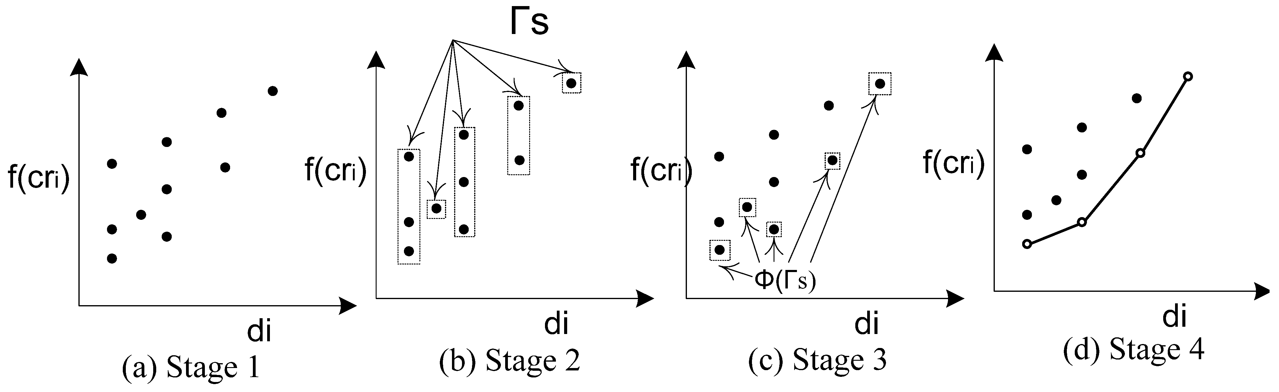
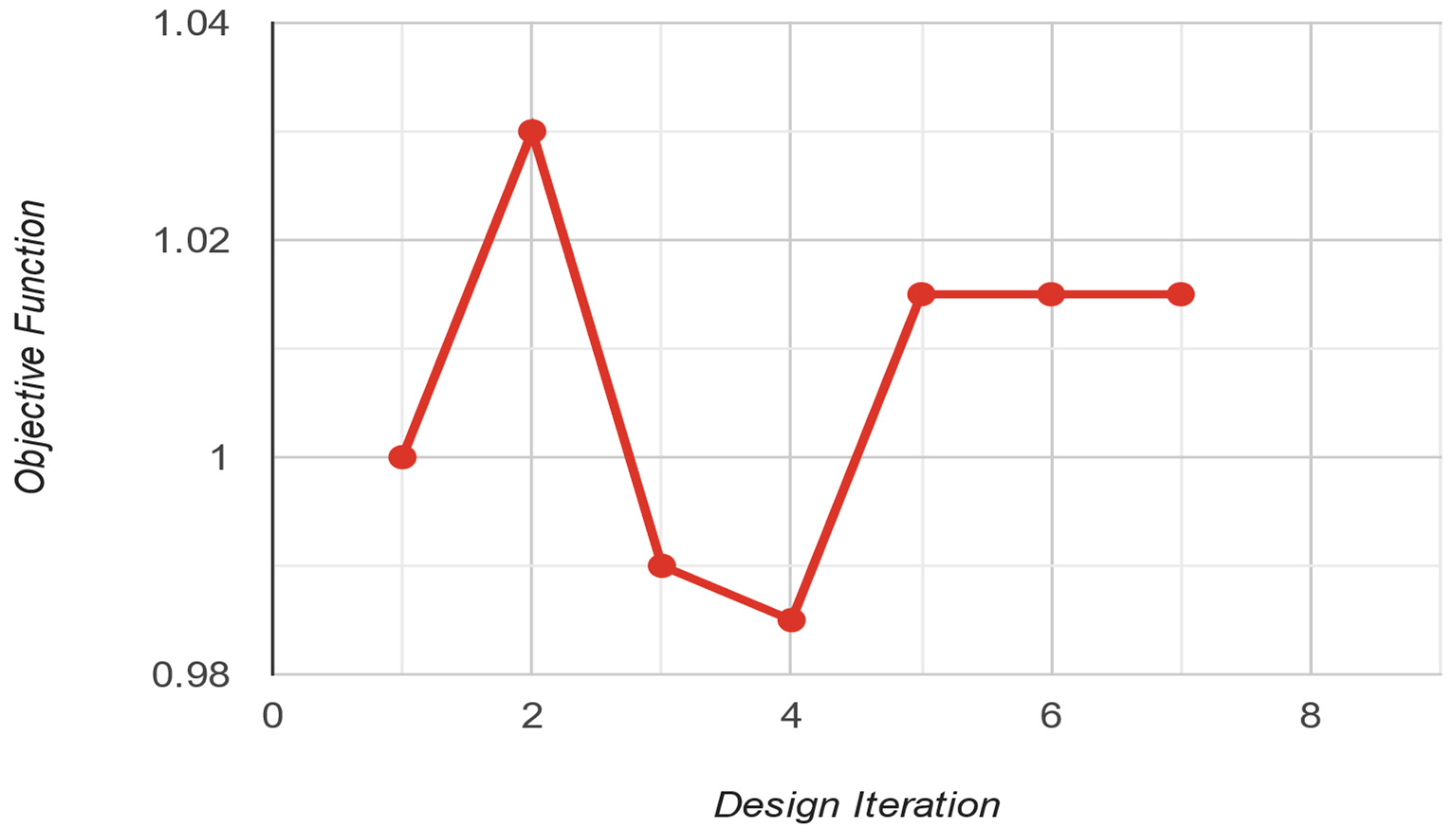
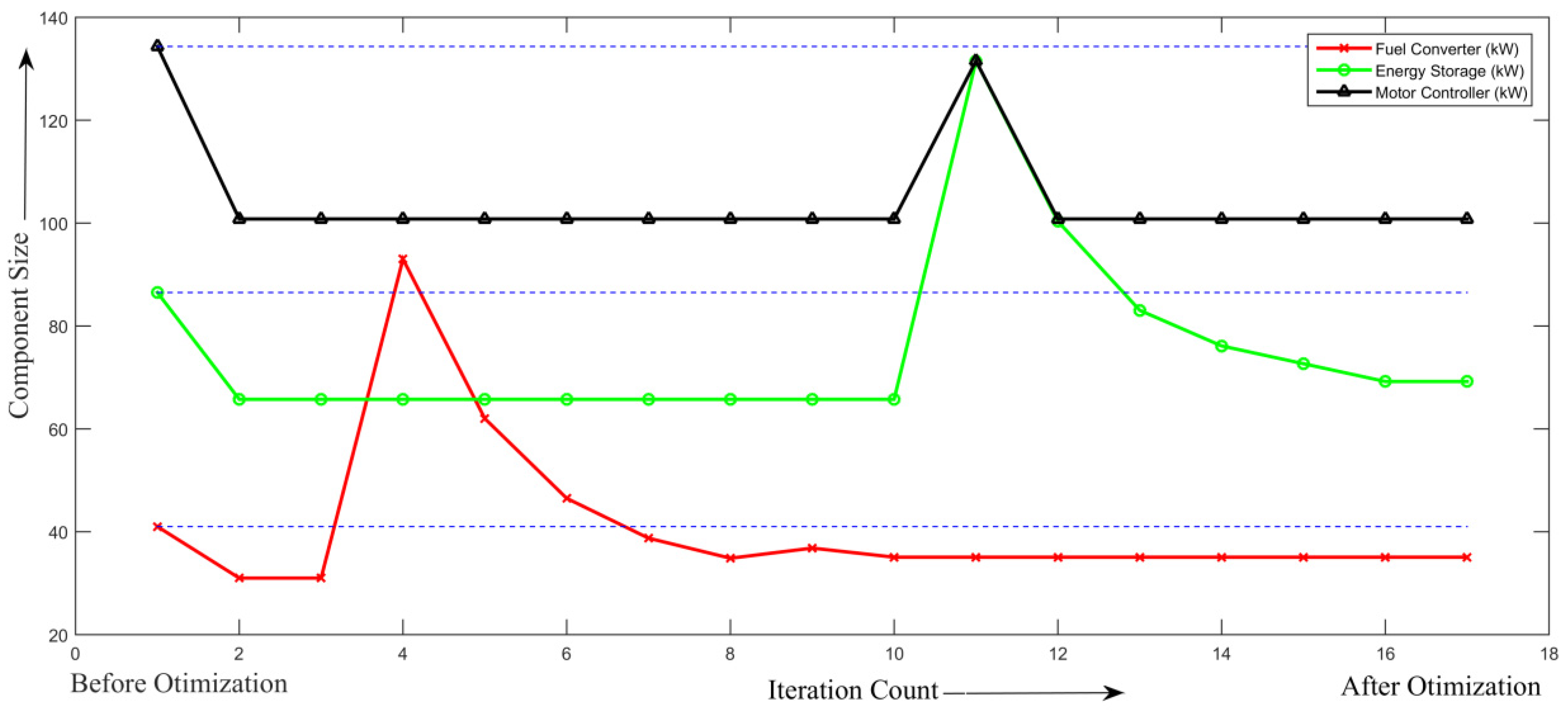
5. Optimization Process
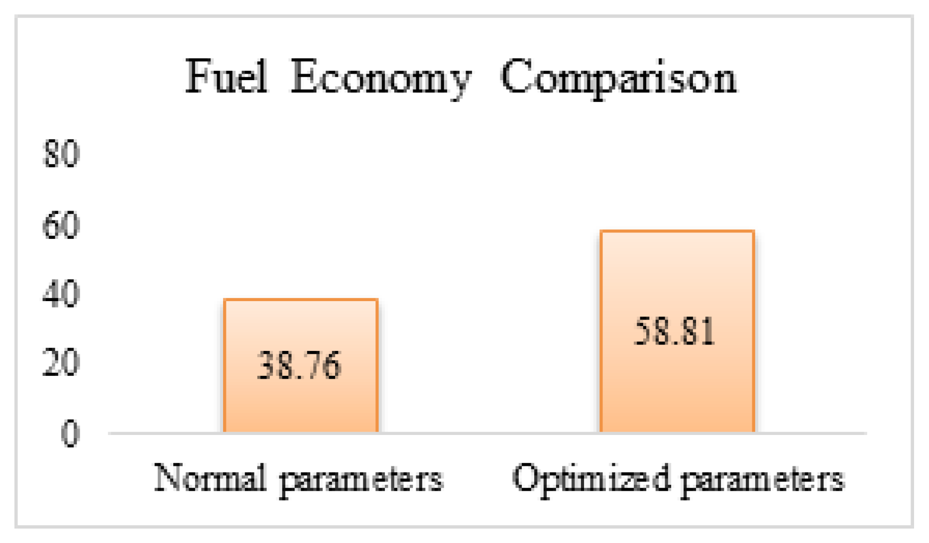
6. Results and Discussion
7. Conclusions
Author Contributions
Funding
Data Availability Statement
Conflicts of Interest
Abbreviations
| Symbol/Abbreviation | Meaning |
| Τ | Torque (Nm) |
| τcrank | Cranking torque (Nm) |
| τaccess | Lumped torque of mechanical accessories (Nm) |
| τcct | Closed throttle torque (Nm) |
| Jeng, Jmotor | Engine and motor inertia (kg) |
| α1, α2, α3, α4 | Coefficients for static friction, Coulomb friction, viscous friction, and air compression torque |
| ω | Angular speed (rad/sec) |
| τref, τdemand | Reference and demanded torque (N-m) |
| τmotor, τregeneration | Motor and regenerative torque (N-m) |
| τspin_loss | Toque loss in spinning (N-m) |
| Pelectrical, Pmechanical | Electrical and mechanical power (kW) |
| Vbus, Vterminal | DC bus and terminal voltage (V) |
| I | Current (A) |
| R | Resistance (Ohm) |
| SOC | State of charge |
| T | Temperature (°C) |
| C | Capacitance (F) |
| Dyn | Dynamic |
| AHr | Ampere hour |
| ƞ | Efficiency |
| CVT | Continuous variable transmission |
| x | State variable |
| u | Control variable |
| Γ | Set of possible hyper-rectangles |
| d | Size of rectangle |
| Φ(Γs) | Hyper-rectangle with best-objective-function value |
| € | Set of all best-objective-function hyper-rectangles |
| cr | Center of objective function |
References
- Mi, C.; Masrur, M.A.; Gao, D.W. Hybrid Electric Vehicles, Principles and Applications with Practical Perspectives; Wiley: Hoboken, NI, USA, 2011; pp. 1–4. [Google Scholar]
- Shafiq, M.; Iqbal, M. Effects of automobile pollutant on the phenology and periodicity of some roadside plants. Pak. J. Bot. 2003, 35, 931–938. [Google Scholar]
- Bhandarkar, D.S. Vehicular pollution, their effect on human health and mitigation measures. Veh. Syst. Dyn. 2013, 1, 33–40. [Google Scholar]
- Graham, L.; Noseworthy, L.; Fugler, D.; O’Leary, K.; Karman, D.; Grande, C. Contribution of vehicle emissions from an attached garage to residential indoor air pollution levels. J. Air Waste Manag. Assoc. 2004, 54, 563–584. [Google Scholar] [CrossRef] [PubMed]
- Drobnik, J.; Jain, P. Electric and Hybrid Vehicle Power Electronics Efficiency, Testing and Reliability. World Electr. Veh. J. 2013, 6, 719–730. [Google Scholar] [CrossRef]
- Lie, T.T.; Prasad, K.; Ding, N. The electric vehicle: A review. Int. J. Electr. Hybrid Veh. 2017, 9, 49–66. [Google Scholar] [CrossRef]
- Cikanek, S.; Bailey, K.; Powell, B. Parallel hybrid electric vehicle dynamic model and powertrain control. In Proceedings of the 1997 American Control Conference, Albuquerque, NM, USA, 6 June 1997; pp. 68–88. [Google Scholar]
- Won, J.-S.; Langari, R.; Ehsani, M. An energy management and charge sustaining strategy for a parallel hybrid vehicle with cvt. IEEE Trans. Control Syst. Technol. 2005, 13, 313–320. [Google Scholar]
- Sun, Z.; Wang, Y.; Chen, Z.; Li, X. Min-max game based energy management strategy for fuel cell/supercapacitor hybrid electric vehicles. Appl. Energy 2020, 267, 115086. [Google Scholar] [CrossRef]
- Khoucha, F.; Benbouzid, M.; Kheloui, A. An optimal fuzzy logic power sharing strategy for parallel hybrid electric vehicles. In Proceedings of the IEEE Vehicle Power and Propulsion Conference, Lille, France, 1–3 September 2010; pp. 1–5. [Google Scholar]
- Li, S.G.; Sharkh, S.M.; Walsh, F.C.; Zhang, C.N. Energy and battery management of a plug-in series hybrid electric vehicle using fuzzy logic. IEEE Trans. Veh. Technol. 2011, 60, 3571–3585. [Google Scholar] [CrossRef]
- Gharibeh, H.F.; Yazdankhah, A.S.; Azizian, M.R.; Farrokhifar, M. Online energy management strategy for fuel cell hybrid electric vehicles with installed PV on roof. IEEE Trans. Ind. Appl. 2021, 57, 2859–2869. [Google Scholar] [CrossRef]
- Hu, X.; Liu, S.; Song, K.; Gao, Y.; Zhang, T. Novel fuzzy control energy management strategy for fuel cell hybrid electric vehicles considering state of health. Energies 2021, 14, 6481. [Google Scholar] [CrossRef]
- Zhao, P.; Wang, Y.; Chang, N.; Zhu, Q.; Lin, X. A deep reinforcement learning framework for optimizing fuel economy of hybrid electric vehicles. In Proceedings of the 23rd Asia and South Pacific Design Automation Conference (ASPDAC), Jeju, Republic of Korea, 22–25 January 2018; pp. 196–202. [Google Scholar]
- Du, G.; Zou, Y.; Zhang, X.; Kong, Z.; Wu, J.; He, D. Intelligent energy management for hybrid electric tracked vehicles using online reinforcement learning. Appl. Energy 2019, 251, 113388. [Google Scholar] [CrossRef]
- Sun, H.; Fu, Z.; Tao, F.; Zhu, L.; Si, P. Data-driven reinforcement-learning-based hierarchical energy management strategy for fuel cell/battery/ultracapacitor hybrid electric vehicles. J. Power Sources 2020, 455, 227964. [Google Scholar] [CrossRef]
- Lee, H.; Kang, C.; Park, Y.-I.; Kim, N.; Cha, S.W. Online data-driven energy management of a hybrid electric vehicle using model-based q-learning. IEEE Access 2020, 8, 84444–84454. [Google Scholar] [CrossRef]
- He, H.; Wang, Y.; Li, J.; Dou, J.; Lian, R.; Li, Y. An improved energy management strategy for hybrid electric vehicles integrating multistates of vehicle-traffic information. IEEE Trans. Transp. Electrif. 2021, 7, 1161–1172. [Google Scholar] [CrossRef]
- Tian, X.; He, R.; Sun, X.; Cai, Y.; Xu, Y. An anfis-based ecms for energy opti- mization of parallel hybrid electric bus. IEEE Trans. Veh. Technol. 2020, 69, 1473–1483. [Google Scholar] [CrossRef]
- Liu, Y.; Liu, J.; Qin, D.; Li, G.; Chen, Z.; Zhang, Y. Online energy management strategy of fuel cell hybrid electric vehicles based on rule learning. J. Clean. Prod. 2020, 260, 121017. [Google Scholar] [CrossRef]
- Tulpule, P.; Marano, V.; Rizzoni, G. Energy management for plug-in hybrid electric vehicles using equivalent consumption minimisation strategy. Int. J. Electr. Hybrid Veh. 2010, 2, 329–350. [Google Scholar] [CrossRef]
- Borthakur, S.; Subramanian, S. Design and optimization of a modified series hybrid electric vehicle powertrain. Proc. Inst. Mech. Eng. Part D J. Automob. Eng. 2018, 233, 1419–1435. [Google Scholar] [CrossRef]
- Dirnberger, M.; Herzog, H.G. A verification approach for the optimization of mild hybrid electric vehicles. In Proceedings of the IEEE International Electric Machines & Drives Conference (IEMDC), Coeur d’Alene, ID, USA, 10–13 May 2015; pp. 1494–1500. [Google Scholar]
- Zhang, F.; Hu, X.; Langari, R.; Wang, L.; Cut, Y.; Pang, H. Adaptive energy management in automated hybrid electric vehicles with flexible torque request. Energy 2021, 214, 118873. [Google Scholar] [CrossRef]
- Zhu, Y.; Chen, Y.; Wu, Z.; Wang, A. Optimisation design of an energy management strategy for hybrid vehicles. Int. J. Altern. Propuls. 2006, 1, 47–62. [Google Scholar] [CrossRef]
- Tian, Y.; Liu, J.; Yao, Q.; Liu, K. Optimal Control Strategy for Parallel Plug-in Hybrid Electric Vehicles Based on Dynamic Programming. World Electr. Veh. J. 2021, 12, 85. [Google Scholar] [CrossRef]
- Adeleke, O.; Li, Y.; Chen, Q.; Zhou, W.; Xu, X.; Cui, X. Torque Distribution Based on Dynamic Programming Algorithm for Four In-Wheel Motor Drive Electric Vehicle Considering Energy Efficiency Optimization. World Electr. Veh. J. 2022, 13, 181. [Google Scholar] [CrossRef]
- Jonathan, N.; Duysinx, P.; Louvigny, Y. Eco-efficiency optimization of hybrid electric vehicle based on response surface method and genetic algorithm. In Proceedings of the EET-2008 European Ele-Drive Conference International Advanced Mobility Forum, Geneva, Switzerland, 11–13 March 2008; pp. 1–10. [Google Scholar]
- Osornio-Correa, C.; Villarreal-Calva, R.; Estavillo-Galsworthy, J.; Molina-Cristóbal, A.; Santillán-Gutiérrez, S. Optimization of power train and control strategy of a hybrid electric vehicle for maximum energy economy. Ing. Investig. Tecnol. 2013, 14, 65–80. [Google Scholar] [CrossRef]
- Ebbesen, S.; Donitz, C.; Guzzella, L. Particle swarm optimisation for hybrid electric drive-train sizing. Int. J. Veh. Des. 2012, 58, 181–199. [Google Scholar] [CrossRef]
- Hegazy, O.; Van Mierlo, J. Optimal power management and powertrain components sizing of fuel cell/battery hybrid electric vehicles based on particle swarm optimization. Int. J. Veh. Des. 2012, 58, 200–222. [Google Scholar] [CrossRef]
- Styler, A.; Nourbakhsh, I. Real-time predictive optimization for energy management in a hybrid electric vehicle. In Proceedings of the Twenty-Ninth AAAI Conference on Artificial Intelligence, AAAI’15, Austin, TX, USA, 25–30 January 2015; pp. 737–743. [Google Scholar]
- Liu, Y.; Gao, J.; Qin, D.; Zhang, Y.; Lei, Z. Rule-corrected energy management strategy for hybrid electric vehicles based on operation-mode prediction. J. Clean. Prod. 2018, 188, 796–806. [Google Scholar] [CrossRef]
- Xu, F.; Shen, T. Decentralized optimal merging control with optimization of energy consumption for connected hybrid electric vehicles. IEEE Trans. Intell. Transp. Syst. 2022, 23, 5539–5551. [Google Scholar] [CrossRef]
- Larmini, J.; Lowry, J. Electric Vehicle Technology Explained; Willey: Hoboken, NI, USA, 2012; pp. 1–10. [Google Scholar]
- Guzzela, L.; Sciarreta, A. Vehicle Propulsion System, Introduction to Modeling and Optimization; Springer: Berlin/Heidelberg, Germany, 2007; pp. 5–15. [Google Scholar]
- Liu, W. Introduction to Hybrid Vehicle System Modeling and Control; John Wiley & Sons: Etobicoke, ON, Canada, 2013. [Google Scholar]
- Rousseau, G.; Sinoquet, D.; Sciarretta, A.; Milhau, Y. Design optimisation and optimal control for hybrid vehicles. Optim. Eng. 2011, 12, 199–213. [Google Scholar]
- Zoelch, U.; Schroeder, D. Dynamic optimization method for design and rating of the components of a hybrid vehicle. Int. J. Veh. Des. 1998, 19, 1–13. [Google Scholar]
- Kleimaier, A.; Schroder, D. Optimization strategy for design and control of a hybrid vehicle. In Proceedings of the 6th International Workshop on Advanced Motion Control, Nagoya, Japan, 30 March–1 April 2000; pp. 459–464. [Google Scholar]
- Markel, T.; Brooker, A.; Hendricks, T.; Johnson, V.; Kelly, K.; Kramer, B.; O’Keefe, M.; Sprik, S.; Wipke, K. ADVISOR: A systems analysis tool for advanced vehicle modeling. J. Power Sources 2022, 110, 255–266. [Google Scholar] [CrossRef]
- ADVISOR Documentation. 2013. Available online: https://adv-vehicle-sim.sourceforge.net/advisor_doc.html (accessed on 8 October 2022).
- Jeanneret, B.; Buttes, A.G.D.; Keromnes, A.; Pelissier, S.; Moyne, L.L. Optimal Control for Cleaner Hybrid Vehicles: A Backward Approach. Appl. Sci. 2022, 12, 578. [Google Scholar] [CrossRef]
- Jeanneret, B.; Guille, D.B.; Pelluet, J.; Keromnes, A.; Pélissier, S.; Moyne, L. Optimal Control of a Spark Ignition Engine Including Cold Start Operations for Consumption/Emissions Compromises. Appl. Sci. 2021, 11, 971. [Google Scholar] [CrossRef]
- Jones, D.R. The DIRECT Global Optimization Algorithm. Encyclopedia of Optimization; Springer: Berlin/Heidelberg, Germany, 2009; pp. 725–735. [Google Scholar]
- Jones, D.R.; Martin, J. The DIRECT algorithm: 25 years Later. J. Glob. Optim. 2021, 79, 521–566. [Google Scholar] [CrossRef]
- Gao, W.; Mi, C. Hybrid vehicle design using global optimisation algorithms. Int. J. Electr. Hybrid Veh. 2007, 1, 57–70. [Google Scholar] [CrossRef]
- Nicholas, P. A Dividing Rectangles Algorithm for Stochastic Simulation Optimization. In Proceedings of the 14th INFORMS Computing Society Conference, Richmond, VA, USA, 11–13 January 2015; pp. 47–61. [Google Scholar]
- Drive Cycle Data. Available online: https://www.nrel.gov/transportation/secure-transportation-data/tsdc-drive-cycle-data.html (accessed on 10 October 2022).


| Variable | Description |
|---|---|
| cs_hi_soc | Highest target battery SOC |
| cs_lo_soc | Lowest target battery SOC |
| cs_electric_launch_spd _hi | Vehicle speed below which pure EV mode is switched on |
| cs_electric_launch_spd _lo | Lowest vehicle speed in pure EV mode |
| cs_off_trq_frac | Minimum torque threshold; when controlled at a lower torque, the ICE will switch off if SOC > cs_lo_soc |
| cs_min_trq_frac | Minimum torque threshold; when controlled at a lower torque, the ICE operates at the threshold torque and the motor works in regenerating mode if the SOC < cs_lo_soc |
| cs_charge_trq | Additional torque required by the ICE for recharging the battery when the ICE is ON |
| Variable Name | Initial Condition | Lower Bound | Upper Bound |
|---|---|---|---|
| cs_lo_SOC | 0.4 | 0.1 | 0.5 |
| cs_hi_SOC | 0.8 | 0.55 | 1 |
| cs_charge_trq | 15.25 | 1 | 80.9 |
| cs_min_trq_frac | 0.4 | 0.05 | 1 |
| cs_off_trq_frac | 0.05 | 0.05 | 1 |
| cs_electric_launch_spd_lo | 0 | 0 | 15 |
| cs_electric_launch_spd_hi | 10 | 10 | 30 |
| Parameter | Goal | Tolerance |
|---|---|---|
| Speed (mph) | 55 | 0.01 |
| Grade (%) | 6 | 0.05 |
| Speed Range | Goal | Tolerance |
|---|---|---|
| 0–18 mph | 3.5 | 0.02 |
| 0–30 mph | 10 | 0.02 |
| 0–60 mph | 12 | 0.02 |
| 40–60 mph | 5.3 | 0.02 |
| 0–85 mph | 23.4 | 0.05 |
| Parameter | Value |
|---|---|
| Drive train | Parallel |
| ICE type | SI |
| Battery | Lead acid (308 V) |
| Motor | AC_75 |
| Transmission | Manual |
| Vehicle mass | 1350 kg |
| Drive Cycle | Before Optimization | After Optimization | Percent Increase |
|---|---|---|---|
| CYC_UDDS | 42.1 | 75.7 | 79.8 |
| CYC_US06 | 36.6 | 39.1 | 6.8 |
| CYC_FTP | 41.9 | 71.5 | 70.6 |
| CYC_INRETS | 36.5 | 44.2 | 21.1 |
| CYC_WVYSUB | 42.5 | 56 | 31.8 |
| CYC_REP05 | 39.7 | 44.9 | 13.1 |
| CYC_OCC | 31.7 | 76.3 | 140.7 |
| CYC_LA92 | 36.6 | 48.6 | 32.8 |
| CYC_ARB02 | 35.8 | 40.4 | 12.8 |
| CYC_India_Hwy | 49.2 | 57 | 15.9 |
| CYC_India_Urban | 33.8 | 93.2 | 175.7 |
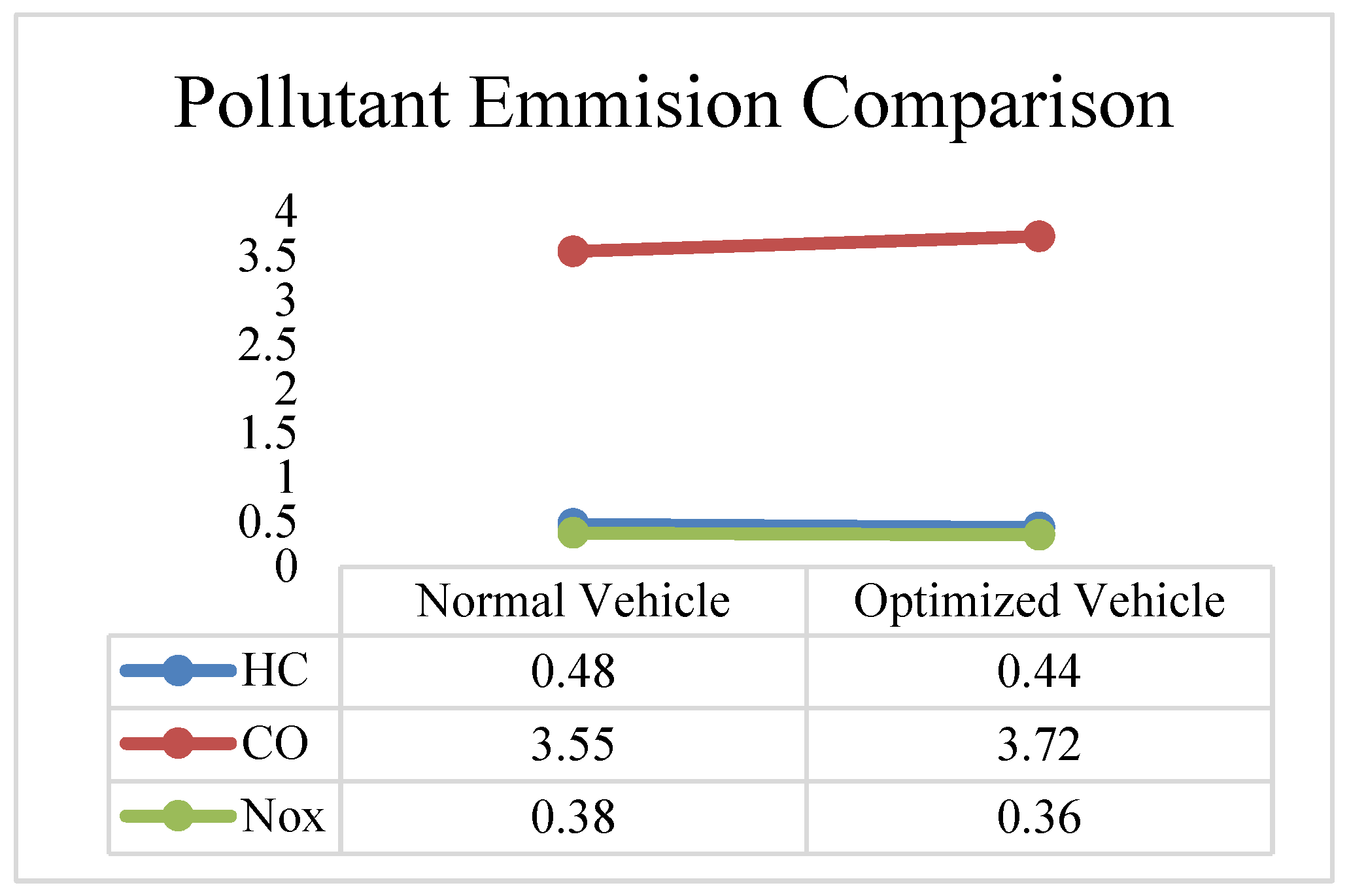
| Drive Cycle | Pollutant | Before Optimization | After Optimization | Percentage Change |
|---|---|---|---|---|
| CYC_UDDS | HC | 0.553 | 0.476 | 13.9 |
| CO | 2.445 | 2.537 | −3.76 | |
| NOx | 0.41 | 0.358 | 12.7 | |
| CYC_US06 | HC | 0.54 | 0.505 | 6.5 |
| CO | 9.07 | 9.625 | −6.1 | |
| NOx | 0.476 | 0.437 | 8.2 | |
| CYC_FTP | HC | 0.416 | 0.372 | 106 |
| CO | 1.978 | 2.155 | −8.9 | |
| NOx | 0.347 | 0.313 | 9.8 | |
| CYC_INRETS | HC | 0.355 | 0.324 | 8.7 |
| CO | 2.304 | 2.452 | −6.4 | |
| NOx | 0.316 | 0.292 | 7.6 | |
| CYC_WVYSUB | HC | 0.568 | 0.546 | 3.9 |
| CO | 2.155 | 2.311 | −7.2 | |
| NOx | 0.386 | 0.392 | −1.5 | |
| CYC_REP05 | HC | 0.305 | 0.282 | 7.5 |
| CO | 4.97 | 5.234 | −5.3 | |
| NOx | 0.295 | 0.265 | 10.2 | |
| CYC_OCC | HC | 0.67 | 0.593 | 11.5 |
| CO | 2.802 | 2.547 | 9.1 | |
| NOx | 0.428 | 0.394 | 7.9 | |
| CYC_LA92 | HC | 0.473 | 0.447 | 5.5 |
| CO | 3.166 | 4.461 | −40.9 | |
| NOx | 0.416 | 0.397 | 4.6 | |
| CYC_ARB02 | HC | 0.325 | 0.291 | 10.4 |
| CO | 5.51 | 5.317 | 3.5 | |
| NOx | 0.324 | 0.303 | 6.5 | |
| CYC_India_Urban | HC | 0.477 | 0.399 | 16.4 |
| CO | 2.15 | 1.846 | 14.1 | |
| NOx | 0.377 | 0.317 | 15.9 | |
| CYC_India_Hwy | HC | 0.582 | 0.573 | 1.5 |
| CO | 2.457 | 2.416 | 1.7 | |
| NOx | 0.447 | 0.501 | −12.1 |
Disclaimer/Publisher’s Note: The statements, opinions and data contained in all publications are solely those of the individual author(s) and contributor(s) and not of MDPI and/or the editor(s). MDPI and/or the editor(s) disclaim responsibility for any injury to people or property resulting from any ideas, methods, instructions or products referred to in the content. |
© 2023 by the authors. Licensee MDPI, Basel, Switzerland. This article is an open access article distributed under the terms and conditions of the Creative Commons Attribution (CC BY) license (https://creativecommons.org/licenses/by/4.0/).
Share and Cite
Srivastava, S.; Maurya, S.K.; Chauhan, R.K. Fuel-Efficiency Improvement by Component-Size Optimization in Hybrid Electric Vehicles. World Electr. Veh. J. 2023, 14, 24. https://doi.org/10.3390/wevj14010024
Srivastava S, Maurya SK, Chauhan RK. Fuel-Efficiency Improvement by Component-Size Optimization in Hybrid Electric Vehicles. World Electric Vehicle Journal. 2023; 14(1):24. https://doi.org/10.3390/wevj14010024
Chicago/Turabian StyleSrivastava, Swapnil, Sanjay Kumar Maurya, and Rajeev Kumar Chauhan. 2023. "Fuel-Efficiency Improvement by Component-Size Optimization in Hybrid Electric Vehicles" World Electric Vehicle Journal 14, no. 1: 24. https://doi.org/10.3390/wevj14010024
APA StyleSrivastava, S., Maurya, S. K., & Chauhan, R. K. (2023). Fuel-Efficiency Improvement by Component-Size Optimization in Hybrid Electric Vehicles. World Electric Vehicle Journal, 14(1), 24. https://doi.org/10.3390/wevj14010024