Unifying Criteria for Calculating the Levelized Cost of Driving in Electro-Mobility Applications

Abstract

The Levelized Cost of Driving (LCOD) calculates how much it costs to drive a vehicle, per kilometer, over the vehicle lifespan, and it is typically measured in USD/km. LCOD has been widely applied to assess and compare the performance of Electric Vehicles (EVs) and Internal Combustion engine Vehicles (ICVs). Unfortunately, there is no common methodology to establish how to compute LCOD. As authors use different criteria to determine which elements are relevant in LCOD, it is difficult to compare results. To overcome this issue, we re-introduce the LCOD concept, where the most relevant expenditures and incomes are included. This novel LCOD definition also incorporates key elements that are sometimes neglected, such as the second life of batteries in EVs, EV battery degradation models, and stochastic models, to characterize daily operation. The proposed methodology is applied to assess the cost of using EVs as taxis in the city of Quito, Ecuador.

1. Introduction

Electric Vehicles (EVs) are currently considered one of the most promising alternatives to Internal Combustion engine Vehicles (ICVs) in the endeavor towards a cleaner transportation sector [1]. The massive usage of these free-emission terrestrial vehicles is starting to become a reality in some countries, such as Norway and Iceland [2], and the total number of EVs around the world has been steadily increasing during the last decade [3]. Despite this positive trend, the worldwide adoption of EVs is still limited compared with conventional automobiles. This phenomenon is attributed to diverse factors including inferior performance, considerable initial cost, and limited charging infrastructure. The high purchase cost is still one of the most important barriers to acquire EVs [4]. Nonetheless, the costs associated with the operation and maintenance of EVs tend to be lower compared with ICVs, which might hence alleviate the initial investment in the long term. Considering the above, one may wonder which vehicular technology (EVs or ICVs) is currently more convenient. To address this question, we need an indicator capable of measuring the performance of one vehicle in economic terms.

The Levelized Cost arises as a natural economic gauge to compare the performance of different vehicular technologies. Levelized Cost aims at determining the cost associated with driving an electric automobile, throughout its entire lifespan, measured in USD/km. Due to its direct interpretability, it has been widely applied to assess the performance of EVs and ICVs [5,6,7,8,9]. The Life Cycle Cost (LCC) is an economic evaluation technique that determines the total cost of owning, operating, and disposing of a system over its lifespan [10,11,12].

Indeed, Ref. [5] determines the Levelized Cost of Driving (LCOD) by taking into account Capital Expenditures (CAPEX) and annual energy consumption expenditures, and assumes that the annual distance traveled is fixed. Jadun et al. in [6] outperforms the LCOD formulation introduced in [5] by incorporating novel relevant factors: Operational Expenditures (OPEX) and efficiency. On the other hand, a more practical analysis is presented in [7], wherein the authors leverage LCOD to compare the economic performance of EVs and ICVs by using real-world data collected by the EV subsidiary program in Beijing. This comprehensive study even encompasses user driving patterns and vehicle age. Finally, perhaps the most complete LCOD implementation is developed in [9] by the National Renewable Energy Laboratory (NREL). The model incorporates numerous inputs such as vehicle type, battery, energy fee, battery lifetime, user driving patterns, and infrastructure costs. Additionally, it describes the EV battery as a function of the operational profile, with the aim of finding a degradation rate per mile. As noted, each of these research efforts takes into consideration dissimilar factors (see

Table 1. Summary of the factors commonly considered for economic analyzes to evaluate electric mobility.

Factor	Reviewed Works
	Levelized Cost (LCOD)					Life Cycle Cost (LCC)					Other Approaches
	[5,6]	[7]	[8]	[9]	Proposal	[13]	[10]	[11]	[12]	[14]	[15]	[16]	[17]
Charging station infrastructure				✓	✓		✓
EV price	✓	✓	✓	✓	✓	✓	✓	✓	✓	✓	✓	✓	✓
Taxes		✓											✓
Depreciation					✓						✓
Maintenance cost	✓	✓	✓	✓	✓	✓	✓	✓	✓	✓	✓	✓	✓
Operational cost	✓	✓	✓	✓	✓	✓	✓	✓	✓	✓	✓	✓	✓
Air emission						✓		✓		✓	✓	✓	✓
Government incentives		✓		✓		✓					✓
Social externalities						✓
Insurance cost		✓		✓	✓	✓			✓
Residual value				✓	✓	✓		✓	✓
Disposal costs					✓			✓	✓
Depth of Discharge (DoD)				✓	✓						✓
Battery price		✓		✓	✓	✓		✓	✓			✓
Battery degradation				✓	✓
Stochasticity of daily operation		✓	✓	✓	✓						✓		✓
Hybrid Electric Vehicles (HEVs)	✓						✓	✓			✓
Battery second life					✓

).

There are certainly other approaches that can also be used to compare different vehicular technologies. For instance, in [15] authors propose a methodology to evaluate the unit-based cost of Electric Vehicles, Hybrid EVs, Plug-in Hybrid EVs, and ICVs. They consider two assessment indices: the first one is focused on the vehicle expenditures, whereas the second measures social impact. On the other hand, Ref. [14] investigate the economic impact of two charging strategies for EVs: (i) conventional approach, in which the recharge is carried out at the station, and (ii) battery swapping, wherein the depleted EV battery is just swapped by a charged one. They analyze how the charging policies could impact the battery lifetime and the long-term costs. In [16,17], the authors examine the feasibility of the massive usage of EVs as taxis in Seoul, South Korea. Finally, in [13], researchers propose an economic indicator called Life-Cycle Private Cost (LCPC), which seeks to calculate the present value of the costs associated with the vehicle operational lifetime. To perform this, they apply the Net Present Value (NPV) approach. Similar to the LCOD implementations discussed earlier, these research efforts incorporate diverse assumptions and factors into the economic analysis, which have been conveniently summarized in Table 1.

Considering the aforementioned information, it can be stated that these analyses lack unified criteria to evaluate EVs from an economic standpoint. This is even more notorious in the case of LCOD-based indicators, because all authors are trying to estimate the same quantity using different considerations. As a consequence, their results are not comparable at all, which is certainly undesirable. To overcome this issue, in this work, we re-introduce the LCOD concept, with a clear orientation to electro-mobility applications, using a unified perspective where the most relevant expenditures and incomes are included. This unified approach also includes key elements sometimes obviated in other approaches: battery second life, EV battery degradation model based on the operational conditions, and stochasticity of the daily operation. In this regard, the main contributions of this work are:

• We re-introduce the LCOD from a unified approach so that findings and results obtained in different research initiatives will be comparable.
• We include some key concepts into the economic analysis that are often obviated: battery second life, EV battery degradation model based on the operational conditions, and stochasticity of the daily operation. Table 1 includes the aspects considered by the proposed LCOD model.

This paper is organized as follows. Section 2 presents the proposed methodology to evaluate the operation of EVs from an economic perspective. Section 3 focuses on the analysis of a case study where the economic feasibility of EVs used as taxis in the South-American city of Quito, Ecuador, is explored. Section 4 presents a summary of the main results and a discussion based on a sensitivity analysis and, finally, Section 5 shows the main conclusions of this research effort.

2. Proposed Methodology for Evaluating Economically the Operation of EVs

To assess the economic performance of a particular vehicular technology, we propose examining the associated implications from a project evaluation perspective to leverage widely-known tools such as NPV. By doing so, our analysis will be focused on investigating the expected cash flows throughout the project life cycle. These cash flows are associated with capital expenditures, maintenance expenditures, and rewards obtained during the daily operation. In this approach, we can suppose that both the vehicle price and maintenance expenditures are fixed, whereas rewards could be variant. These assumptions trigger the following question: what is the minimum reward per kilometer that guarantees the feasibility of the project? This lower bound for rewards is informative regarding the economic performance of the vehicle when used in a specific application; therefore, it constitutes a valid economic indicator. Motivated by the previous insights, the Levelized Cost of Driving (LCOD) arises as an economic indicator that systematically addresses the above question; it is formally derived in the following paragraphs from a unified perspective.

Considering these aspects, let us initiate the proposed procedure by computing the NPV:

$$\begin{array}{cc}\hfill \mathrm{NPV}=-\mathrm{CAPEX}+\sum _{t=1}^n& \left(\frac{I_t-{\mathrm{OPEX}}_t}{{(1+r)}^t}\right)+\frac{\mathrm{RV}}{{(1+r)}^n}-\sum _{tc=1}^{nc}\frac{\mathrm{DC}+\mathrm{RC}}{{(1+r)}^{yc}}\hfill \end{array}$$

(1)

The NPV is evaluated at a fixed horizon equal to n years with a discount rate r. As usual, the NPV includes Operational Expenditures (OPEX), Capital Expenditures (CAPEX), incomes (I), Residual Value (RV), and the Reparation Cost (RC). Disposal Costs (DC) is the cost of recycling the EV batteries. The formulation allows to consider an RV of the vehicle at the end of the project. When there is a battery replacement in the EV or engine repair in the ICV, it is considered an RC and a DC in the year (yc) that the change is made. The sum of the amount (nc) of the RC and DC is made during the life of the project.

It is also relevant to observe that in (1) the income can be described as a reward per kilometer traveled, which is denoted as $\lambda$ [USD/km]. With this definition, the incomes collected during the year t can be rewritten as $\lambda$ · KM${}_t$, where KM${}_t$ is the distance in kilometers traveled during year t. Subsequently, we can now calculate the minimum $\lambda$ that guarantees the project feasibility. To do this, we replace $I_t$ by $\lambda$ · KM${}_t$ in (1), and afterward solve NPV$\left(r\right)=0$. By doing so, the solution of this equation is, by definition, the proposed indicator LCOD. Finally, we can derive a closed-form expression of LCOD resulting in the following:

$$\mathrm{LCOD}:=\frac{\mathrm{CAPEX}-\frac{\mathrm{RV}}{{(1+r)}^n}+{\sum }_{tc=1}^{nc}\frac{\mathrm{DC}+\mathrm{RC}}{{(1+r)}^{yc}}+{\sum }_{t=1}^n\frac{{\mathrm{OPEX}}_t}{{(1+r)}^t}}{{\sum }_{t=1}^n\frac{{\mathrm{KM}}_t}{{(1+r)}^t}}$$

(2)

Although the LCOD derivation is general, the computation of each of the terms related to its definition will depend on the particular vehicular technology under evaluation. As examples, in the following subsections (Section 2.1, Section 2.2 and Section 2.3), the determination of these quantities for the case of EVs and ICVs will be explored from the LCOD perspective. In this regard, it will be relevant to focus the analysis on the EVs and ICVs in Section 3 wherein both technologies will be compared economically with one application related to taxis by the proposed LCOD indicator. Moreover, Section 2.4 also presents a detailed discussion on how to incorporate the stochasticity of the daily operation of vehicles into the LCOD analysis.

2.1. CAPEX

CAPEX constitutes the initial capital investment to buy a vehicle. Consequently, it solely depends on the vehicle market price.

2.2. Residual Value and Reparation Cost

After finishing the project, the vehicle may still be useful and thus have a commercial value, which is known as the residual value. This value may increment notably if the vehicle is repaired, hence we consider a final Reparation Cost (RC) as well. At this point, we must distinguish between EVs and ICVs. In the case of EVs, their battery may be almost completely degraded at end of the project; therefore, the RC${}_{ev}$ will be equal to the price of a new battery (B) plus some mechanical adjustments(MA${}_{ev}$), then:

$${\mathrm{RC}}_{ev}=B+{\mathrm{MA}}_{ev}.$$

(3)

On the other hand, in the case of ICVs, the RC will include just mechanical adjustments, thus RC${}_{icv}$ = MA${}_{icv}$.

Furthermore, for EVs, we acknowledge that the degraded battery is not simply discarded, but sold so that it may be used as energy storage in other applications. This concept is known as battery second life and aims at re-purposing degraded batteries [18,19]. In other words, when a battery is considered degraded at one application (e.g., EVs), it can still be useful for a less-demanding application (e.g., domestic usage). Due to the above, in the case of EVs, we assume that the total residual value can be computed as RV = RV${}_{ev}$ + RV${}_{bat}$, where RV${}_{ev}$ is the residual value of the EV with the new battery and RV${}_{bat}$ corresponds to the residual value of the degraded battery.

2.3. Operational Expenses (OPEX)

The annual Operational Expenses (OPEX) is the result of the sum of two expenses: annual maintenance cost (aMC${}_t$) and annual energy consumption cost(ECC${}_t$), i.e., OPEX${}_t$ = aMC${}_t$ + ECC${}_t$. In the case of ICVs, the annual maintenance cost has this form:

$$a{\mathrm{MC}}_t^{ICV}=K_{ICV}·{\mathrm{KM}}_t+\mathbb{1}({\mathrm{CKM}}_t-{\mathrm{KM}}_{max})·Re{p}_{ICV}.$$

(4)

The first addend represents an annual maintenance cost proportional to the kilometers traveled, where $K_{ICV}$ [USD/km] is the maintenance fee. On the other hand, the second addend indicates that if the cumulative kilometers traveled CKM${}_t$, measured from the last reparation, exceeds a threshold KM${}_{max}$, then the automobile will require a major reparation whose cost is $Re{p}_{ICV}$. Notice that $𝟙\left(x\right)=1$ if $x\ge 0$ and $𝟙\left(x\right)=0$ otherwise. Although in EVs the maintenance cost is usually lower, we must incorporate the possibility of the EV battery getting degraded prematurely before project completion. In such a scenario, it must be replaced, which leads to an expenditure equal to the cost of a new battery B. Consequently,

$$a{\mathrm{MC}}_t^{Ev}=K_{EV}·{\mathrm{KM}}_t+B·𝟙(0.8-{SOH}_t),$$

(5)

where $K_{EV}$ [USD/km] is the EV reparation cost and the other addend corresponds to battery replacement costs. This cost is nonexistent if the battery State-of-Health (SOH) is greater than 80% by the end of the year t; otherwise, it is equal to B. The threshold 80% is chosen because experts suggest that the batteries are no longer useful for traction purposes after they have lost a 20% of their capacity [20,21,22].

Remark 1.

A robust model to forecast the EV battery degradation process is of utmost importance to fulfill a solid economic analysis in the field of EVs, and thus to apply the proposed LCOD indicator. On the contrary, if we adopt a simplistic degradation model, its prediction might indicate that the battery will not get degraded during the project life cycle. Nonetheless, in practice, the battery could get degraded in the middle of the project execution, which may result in a substantial unexpected expenditure that was not contemplated whatsoever in the initial economic analysis. Therefore, the utilization of a detailed battery degradation model that allows to compute reliable predictions is strongly recommended. Such a model should account for several critical factors that govern the EV battery degradation process, such as discharge rate, Depth of Discharge (DoD), temperature, among others [23]. In addition to this, we need to characterize the EV daily usage profile, for example in terms of the daily distance traveled and average speed, because this profile defines the typical current profile delivered by the battery, which in turn impacts its degradation process, as mentioned previously.

Looking at the annual energy consumption cost, ECC${}_j$ varies depending on the price of the energy consumed during the year ${}_t$, then:

$${\mathrm{ECC}}_t=\sum _{i=1}^{N{r}_t}{E}_i·e{f}_i,$$

(6)

where $N{r}_t$ corresponds to the total number of recharges during the year ${}_t$, $E_i$ (expressed in [kWh] in the case of EVs and [GL] for ICVs) represents the magnitude of the recharge when the EV is connected to the power supply or the refuel in the case of ICVs.; and $e{f}_i$ (expressed in USD/kWh and USD/GL for EVs and ICVs, respectively) is the energy fee. Hence, we need to know in advance the number of annual recharges to calculate ECC${}_t$; unfortunately, it is unfeasible in practice due to the stochasticity associated with the daily operation of vehicles. A recommended procedure to overcome this challenge is to characterize the daily distance traveled by the vehicle at the application under study, and then infer energy consumption based on the distance traveled.

2.4. Dealing with the Stochasticity of Daily Vehicle Operation by Monte Carlo Simulation

As noted in Section 2.3, which focused on the analysis of operational expenses, OPEX directly depends on the operational conditions and usage patterns associated with the vehicle. Indeed, when a vehicle is used more aggressively, it degrades more quickly and spends more energy; consequently, its owner will incur higher annual costs. Unfortunately, if at the time of the economic evaluation we are unable to know in advance the exact operating conditions at which the vehicle will be exposed, then computing the OPEX is not straightforward. We propose dealing with this issue by using a Monte Carlo simulation to recreate probable scenarios of future operation and determine the associated LCOD. The underlying idea is to simulate the daily operation of $N_r$ (where $N_r$ is large enough) vehicles and to collect the individual annual OPEX to estimate the stochasticity of this variable. By carrying out this procedure, we can estimate the LCOD for each of these vehicles, and then obtain an approximation to the Probability Density Function (PDF) of the LCOD. This PDF is informative about the variability of the LCOD, and thus helps us to perform a more reliable economic evaluation. The complete simulation procedure is more formally explained in Algorithm 1. It simulates the daily operation of the vehicles for $365·N_y$ (Lines 3–9), where $N_y$ is the project lifetime. For each vehicle, for each day, it samples the distance traveled from ${\mathcal{P}}_{dist}$ (Line 4), which should be estimated based on historical data. Afterward, it saves the daily degradation and energy consumption (Line 5–6), which enables to compute the annual OPEX at the end of each year (Line 7–9). Finally, the LCOD for each vehicle simulated is saved (Line 10). According to the theory behind Monte-Carlo-based procedures, when $N_r$ is large enough, the histogram obtained from the collection of LCOD${}_i$ permits us to approximate the LCOD PDF. Last but not least, sensitivity analyses were performed using the Multi-Objective Optimization using Genetic Algorithms function, in MATLAB, to find the Pareto front of the LCOD with respect to the variable under analysis.

Algorithm 1 Monte Carlo simulation to predict the LCOD probability distribution

Inputs: ${\mathcal{P}}_{dist}:$ Distribution of the distance traveled daily by the vehicles.

Output: LCOD: The final LCOD for each vehicle simulated.

1: for$i=1,\cdots ,N_r$do

2:    $year=0$

3:    for $j=1,\cdots ,365·N_y$ do

4:        $d_j{\mathcal{P}}_{dist}$▹ Sample distance traveled from ${\mathcal{P}}_{dist}$

5:        $de{g}_j\leftarrow$ Calculated daily degradation based on $d_j$

6:        $ec{c}_j\leftarrow$ Compute consumption cost based on $d_j$

7:        if j is the last day of the year then

8:           $year=year+1$

9:           OPEX${}_{year}^j\leftarrow$ Calculate OPEX based on the annual realizations of $de{g}_j$ and $ec{c}_j$.

10:    LCOD${}_i\leftarrow$ Compute LCOD considering OPEX${}_{year}^j$, using Multi-Objective Genetic Algorithm optimization to find the Pareto front.

11: return$LCOD$

Remark 2.

Notice that the LCOD methodology is generic and can be used for both taxis and privately owned vehicles. The user just needs to characterize the daily distance traveled because this quantity directly impacts the OPEX.

3. Case Study: Evaluating the Economic Feasibility of EV Taxis in the City of Quito, Ecuador

Nowadays the Ecuadorian government is seriously evaluating the massive usage of EVs as taxis in Quito, the capital of Ecuador. The implementation of this policy may be notably beneficial to the community from the environmental-care perspective, however, the economic impact is not clear enough. Motivated by the above, in this case study, we will apply LCOD to contrast EVs and ICVs operating as taxis in Quito with the objective of determining which vehicular technology is more convenient. This case of study is also pertinent because several countries are studying pilot projects for the transition from conventional taxis to electric vehicles.

As discussed in Section 2.4, to compute a more reliable estimation of the actual LCOD, it is essential to characterize the distance traveled daily by the vehicles in the application under study. Consequently, we need to statistically represent the distance traveled, daily, by taxis in Quito. To accomplish this, the distribution of total travel distance was first approximated by fitting a non-parametric probability density function (PDF) to measurements collected in a real-world database [24]. The PDF fit result is depicted in Figure 1. Notice that the mean and the standard deviation of the data are 146.1 km and 34.6 km, respectively, whereas the mean and the standard deviation of the fit are 145.6 km and 36.2 km, respectively.

Furthermore, the parameters of the LCOD procedure utilized in this case study were adjusted to represent the Ecuadorian vehicle market (see

Table 2. Case study parameters.

LCOD Parameters	EV	ICV
Economic Parameters
CAPEX [USD]	$39,990	$20,000
Residual Value (RV)	$20,000	$10,000
Battery price (B) [USD]	$8000	-
RC${}_{ICV}$ [USD]	-	$2000
K [USD/km]	$0.025	$0.05
DC [USD]	$-	$-
Technical features
Battery capacity [kWh]	40	-
EV range [km]	280	-
Expected battery lifetime [# cycles]	1000	-
ICV performance in the City [km/GL]	-	45
EV performance in the City [km/kWh]	7.04	-
KM${}_{max}$ [1000 km]	-	400
Energy consumption fee
Electric fee [USD/kWh]	$0.17	-
Fuel fee [USD/GL] (85 & 92 octane)	-	$2.55–$4.66
NPV parameters
Discount rate	10% and 12%

). The vehicles compared in this study are the following:

• EV: NISSAN LEAF 100% Electric, Autonomy: 280 km, Power: 147 hp, Battery capacity 40 kWh, 0.142 kWh/km, 2021 Year.
• ICV: Data sheet ICV: KIA RIO Sedan vehicle cylinder capacity: 1.4 L MPI $4\times 2$, Vehicle performance in the city: (12.1 km/lt), 2021 Year.

Two different fuel fees found in Ecuador are analyzed, 2.55 USD/GL and 4.66 USD/GL, which correspond to the current subsidized prices for the fuel of 85 and 92 octane, respectively.

Disposal Costs (DC) is not considered in this case study because there is still no regulation in Ecuador for the handling and recycling costs of EV batteries.

The EV charging cost depends on where and when the battery is charged. Two recharge options are considered: charging at home and using a charging station. Regarding the charging station tariff price, the Government of Ecuador, based on the provisions of the Organic Law on Energy Efficiency, is working to establish a maximum price (price cap) for fast charging for charging stations, which is estimated to be a value of 0.17 USD/kWh. On the other hand, for EV charging at homes, according to Ecuador Agency of Regulation and Control of Energy (https://www.controlrecursosyenergia.gob.ec/servicio-publico-de-energia-electrica-spee/, (accessed on 1 February 2022)), there is a fixed monthly cost of 4 USD/kW due to demand rate and a variable hourly rate described as follows: from 8:00 to 18:00 it is 0.08 USD/kWh, from 18:00 to 22:00 it is 0.10 USD/kWh, and from 22:00 to 8:00 it is 0.05 USD/kWh. For analysis purposes, we assume that the electricity price is 0.17 USD/kWh, which corresponds to the highest fee—utilizing just charging stations. We also conduct a sensitivity analysis with respect to the electricity price, accounting for the other possible fees.

To forecast the battery degradation process, we adopt the degradation model presented in [25], since it allows us to incorporate the charging policy into the simulation procedure, and hence to reproduce more realistic scenarios. Besides, this model has shown promising results [23,26,27] despite its simplicity. The model assumes that the battery capacity evolves cycle by cycle according to the following expression:

$$C_{k+1}={\eta }_k(So{C}_k^{min},So{C}_k^{max})·C_k,$$

(7)

where C is the battery capacity and ${\eta }_k\in (0,1)$ is the Coulomb efficiency. The latter quantity is dependent on the State-of-Charge (SoC) variation at cycle k and can be tuned for a particular battery following the instructions presented in [25]. Additionally, in our simulations, we suppose that the EV battery will always be recharged when its SoC is less or equal than 20%.

Remark 3.

The EV battery degradation model utilized in the simulation framework should be not only robust but also versatile to be tuned directly through the information provided by the battery datasheet. We highlight this point because the academia offers abundant methodologies to forecast the battery capacity fade, including for instance methods based on electric circuits [28,29,30,31] or electrochemistry [32,33,34]. However, tuning such models demands a huge number of experiments, which are impossible to conduct at the economic evaluation step because we do not even have the vehicle yet. Therefore, our best alternative is to go for methods capable of being tuned based on the information provided by the battery manufacturer such as [25].

4. Case Study: Obtained Results and Sensitivity Analysis

Firstly, we use LCOD to assess the performance of both EVs and ICVs as taxis in Quito, Ecuador. To perform this task, we compute a Monte Carlo simulation with ${10}^3$ instances, according to the procedure described in Section 2.4. The corresponding results are summarized in

Table 3. LCOD result obtained from a Monte Carlo simulation with ${10}^3$ realizations.

	Mean ($\mathit{r}=8$%) [USD/100 km]	Mean ($\mathit{r}=10$%) [USD/100 km]	Mean ($\mathit{r}=12$%) [USD/100 km]
EV LCOD	20.55	21.75	23.03
ICV LCOD [2.55 USD/GL]	17.68	18.38	19.09
ICV LCOD [4.66 USD/GL]	22.36	23.07	23.78

for three different discount rate values: r = 8%, r = 10%, r = 12%. On the one hand, we observe that when the refueling cost in ICVs is assumed to be 2.55 USD/GL, the EV LCOD exceeds the ICV LCOD in 2.87 USD/100 km, 3.37 USD/100 km, 3.94 USD/100 km for each of those discount rates, respectively, which is equivalent to a 15.5% of excess, on average, with respect to the ICV LCOD. On the other hand, we observe that when the refueling cost in ICVs is assumed to be 4.66 USD/GL, the ICV LCOD exceeds the EV LCOD in 2.08 USD/100 km, 1.32 USD/100 km, 0.75 USD/100 km for each discount rate, considered in the analysis, which is equivalent to 5.61% excess, on average, with respect to the EV LCOD. The EV LCOD results are equivalent to the value of ICV LCOD considering a fuel cost of 4.66 USD/GL. Therefore, the operation of an EV as a taxi in this city may be cheaper, the same, or even more expensive compared with the utilization of ICVs, depending on the fuel cost in the locality. It must be also noted that this statement is naturally based on actual fuel prices and, thus, it is always recommended to repeat this financial analysis with up-to-date data before reaching a definitive conclusion in the future.

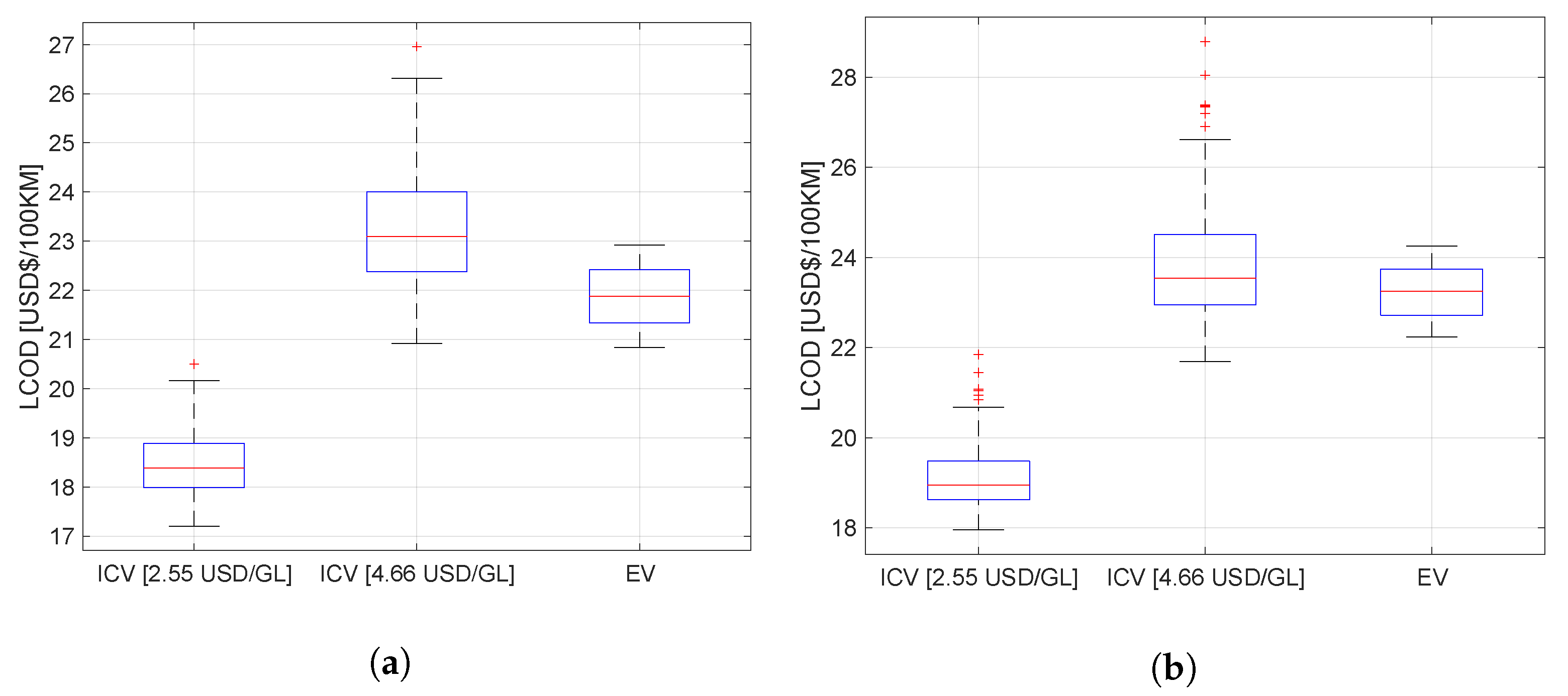
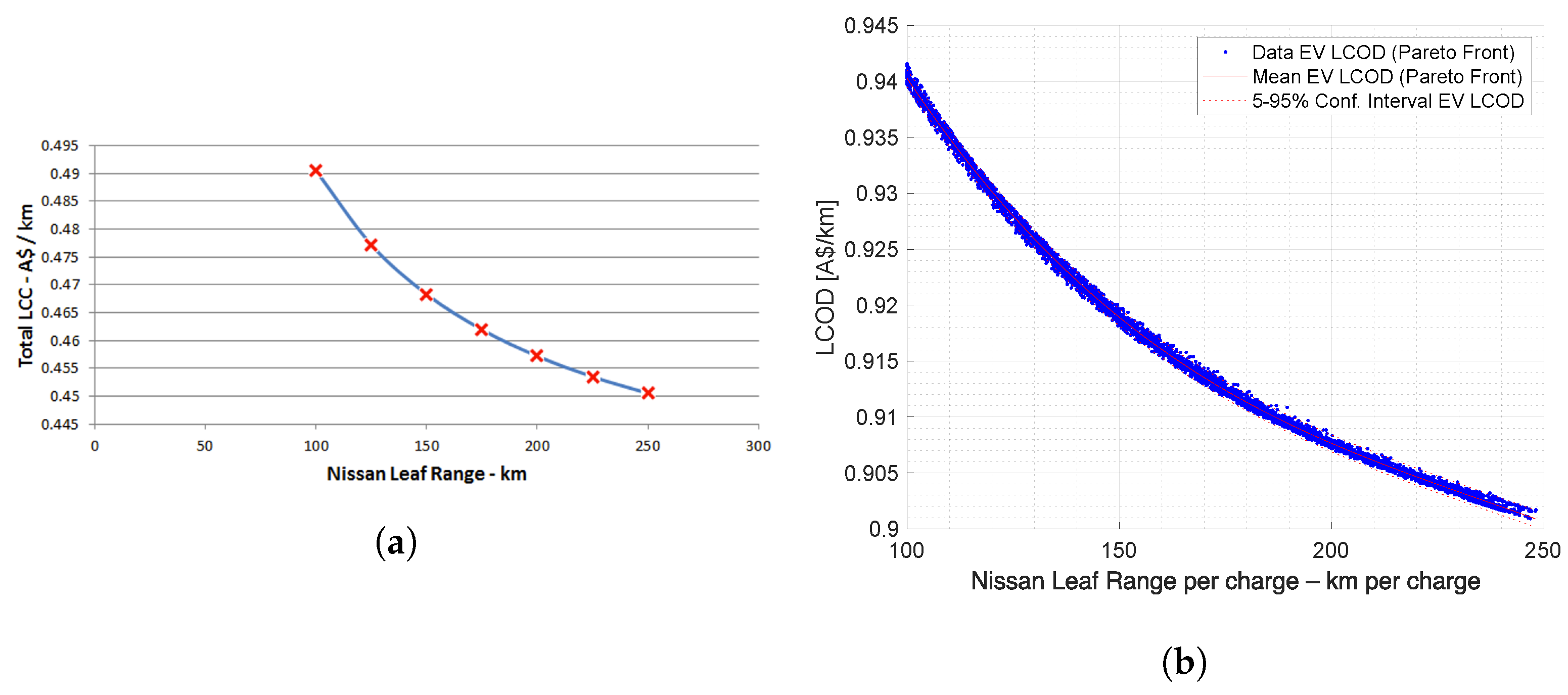
4.1. Sensibility Analysis with Respect to Vehicle Performance

Another key factor to keep in mind when computing the LCOD is the Vehicle Specific Fuel Consumption (VSFC), defined as a ratio between the distance traveled and the corresponding energy consumed over this distance. This quantity is hence measured in km/GL and km/kWh for ICVs and EVs, respectively. Since VSFC can vary depending on the profile use of the vehicle and the characteristics of the route (road, urban streets, or highway), we conducted a sensitivity analysis over this quantity using a Monte Carlo simulation. We suppose that the VSFC for the IC can be modeled by a normal random variable with a mean of 45 km/GL and a standard deviation of 5 km/GL. Similarly, for the EV, we suppose that its VSFC follows a normal random variable with a mean of 7 km/kWh and a standard deviation of 2.5 km/kWh. Subsequently, we proceed to sample from these distributions and for each sample we compute the LCOD. The results obtained are depicted in Figure 2a,b for discount rates $r=10$% and $r=12$%, respectively.

Regarding the estimates for annual average operational expenses (annual average OPEX), obtained results are shown in

Table 4. Annual OPEX Statistics.

	Mean (OPEX) [USD]	Standard Deviation [USD]
EV	2402.3	87.39
ICV [2.55 USD/GL]	4872.9	70.07
ICV [4.66 USD/GL]	7015.0	100.87

. It is noteworthy that EV-related costs represent $49.3$% of ICVs, when considering 2.55 USD/GL, or $34.24$% of ICVs when considering 4.66 USD/GL instead.

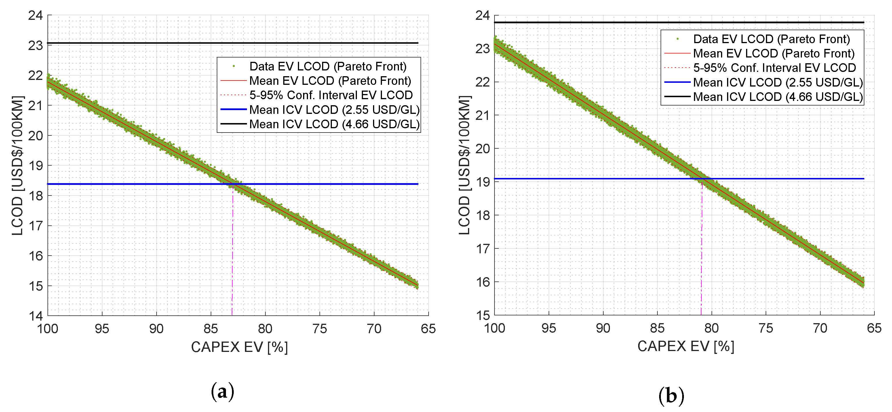
4.2. Sensibility Analysis with Respect to EV CAPEX

To generate the results above, we supposed that CAPEX of the EV was fixed and equal to USD 39,990. Nevertheless, this initial cost might diminish, for example, as a result of government subsidies or new battery technologies. In fact, since several nations are investing in these types of vehicles with the objective of alleviating greenhouse gas emissions, as well as the industry of EVs reducing costs notably, these two potential causes seem reasonable. Aiming at determining the impact of EV CAPEX reductions on the EV-LCOD, we build a sensibility by applying the Pareto front with respect to this variable with ${10}^3$ realizations. This result is depicted in Figure 3a,b for discount rates $r=10$% and $r=12$%, respectively. As expected, it evidences that EV LCOD is directly proportional to the EV CAPEX. In particular, if $r=10$% is assumed, a 17% reduction in EV CAPEX for the scenario where refueling cost in ICVs is 2.55 USD/GL, implies that both vehicular technologies (EV and ICV) have the same performance in terms of LCOD. On the other hand, if $r=10$% in a scenario where the refueling cost in ICV is 4.66 USD/GL, EV technology is cheaper than ICV.

Analogously, if $r=12$% is assumed, a 19% reduction in EV CAPEX for the scenario where refueling cost in ICVs is 2.55 USD/GL implies that both vehicular technologies (EV and ICV) have the same performance in terms of LCOD. On the other hand, if $r=12$%, in a scenario where the refueling cost in ICV is 4.66 USD/GL, EV technology is cheaper than ICV. We should remark that this metric solely regards financial countable costs, but not other positive externalities of EVs, such as its contribution in mitigating both air and acoustic pollution, which are well-known incentives that boost the proliferation of such automobiles.

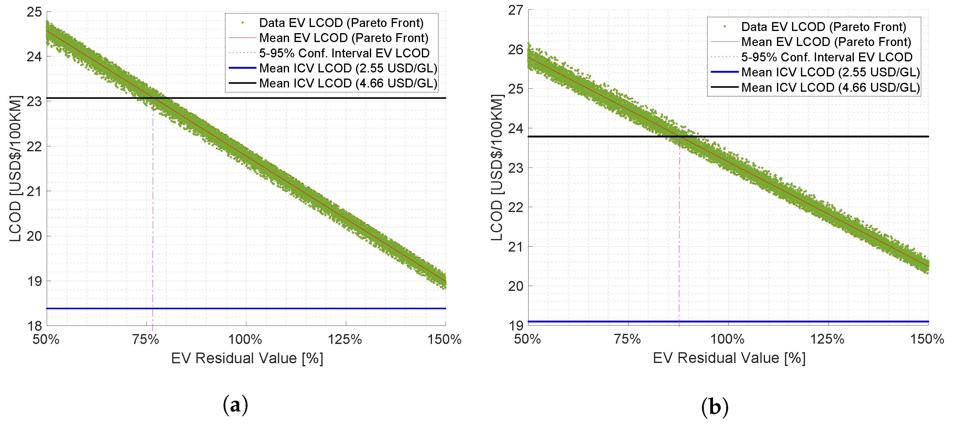
4.3. Sensibility Analysis with Respect to EV Residual Value

On the other hand, in the first results of Table 3, we also assumed that the EV Residual Value (RV) was fixed and equal to USD 20,000. However, since the introduction of EVs to the vehicle market is still recent, the depreciation of such automobiles is a matter of ongoing research [35]; thus, determining the RV of EVs is not straightforward. In particular, our study assumed an annual depreciation rate of 10%. Additionally, we have to acknowledge that the market of batteries to second life, which certainly boosts the EV RV, is still complicated to characterize. The above encouraged us to perform another sensibility analysis by applying the Pareto front with respect to the EV residual value with ${10}^3$ instances; the obtained results can be seen in Figure 4a,b for discount rates $r=10$% and $r=12$%, respectively. In this case, we distinguish naturally that as the EV residual value increases, the gap LCOD between both vehicular technologies is lower. Particularly, if $r=10$% is assumed, a 23% decrease in EV RV for the scenario where refueling cost in ICVs is 4.66 USD/GL implies that both vehicular technologies (EV and ICV) have the same performance in terms of LCOD. A similar outcome is obtained when assuming $r=12$% and a 12% decrease in EV RV for the scenario where refueling cost in ICV is 4.66 USD/GL.

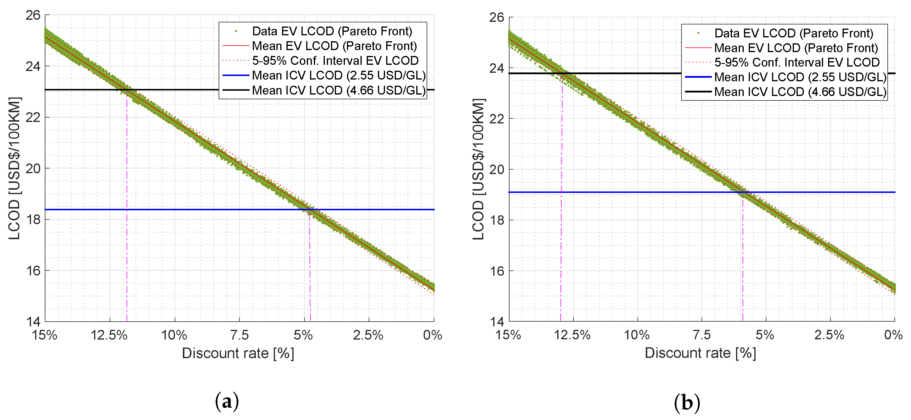
4.4. Sensibility Analysis with Respect to EV the Discount Rate

It must be noted that to generate the results illustrated in Table 3, it was assumed that the discount rate EV (DR) was fixed and equal to 10% and 12%. However, in the determination of DR, many variables enter the financial situation of each country, so determining the DR of electric vehicles is not easy. This fact motivates another sensitivity analysis, where the Pareto front is applied with respect to the EV discount rate. Obtained results for this additional sensitivity analysis are shown in Figure 5a,b. In this case, we naturally distinguish that as the EV discount rate increases, the EV’s LCOD grows. In particular, if $r=10$% and refueling cost for ICV is 4.66 USD/GL, if the EV discount rate is 11.86%, it implies that both vehicle technologies (EV and ICV) perform the same in terms of LCOD. A similar conclusion can be obtained when assuming $r=10$%, the refueling cost for ICV is 2.55 USD/GL, and the EV discount rate is 4.8%.

Similarly, if $r=12$% is assumed and refueling cost for ICV is 4.66 USD/GL, if the EV discount rate is 13%, it implies that both vehicle technologies (EV and ICV) perform the same in terms of LCOD. A similar conclusion can be obtained when assuming $r=12$%, refueling cost for ICV is 2.55 USD/GL, and the EV discount rate is 5.9%.

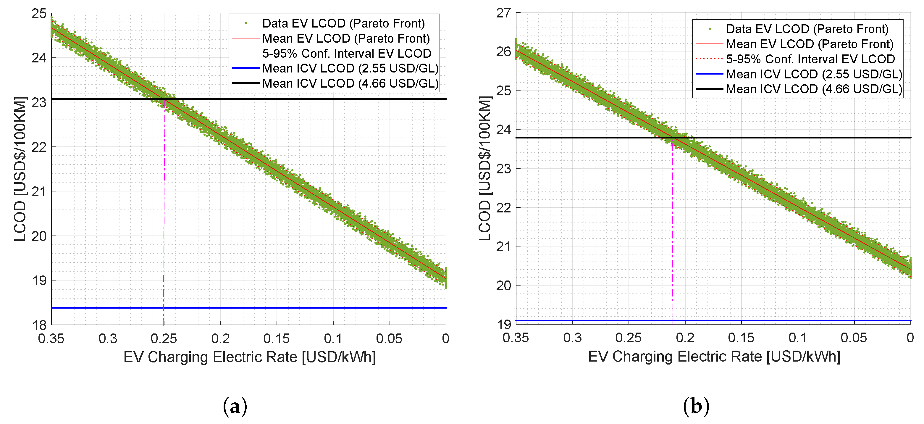
4.5. Sensibility Analysis with Respect to EV Charging Electric Rate

Accounting for the possibility of different electricity prices as described in Section 3, we have included one additional sensitivity analysis (see Figure 6a,b) in terms of the Charging Electricity Rate that considers a single monomic value from 0.0 to 0.35 USD/kWh and two different discount rates ($r=10$% and $r=12$%). When $r=10$% is assumed and refueling cost for ICV is 4.66 USD/GL ( see Figure 6a), we note that setting the EV Charging Electric Rate at 0.25 USD/kWh implies that both vehicle technologies (EV and ICV) perform the same in terms of LCOD. On the other hand, when $r=12$% is assumed and refueling cost for ICV is 4.66 USD/GL ( see Figure 6b), we observe that setting the EV Charging Electric Rate to 0.21 USD/kWh would imply that both vehicle technologies (EV and ICV) perform the same in terms of LCOD.

4.6. Impact of Bias in Battery Degradation Models in Financial Analysis

Last but not least, we have examined the impact of the bias that could exist in battery degradation models on the financial analysis outcome. To perform this sensitivity analysis, we compute the LCOD for a six-year project using two different degradation models for a battery with an estimated lifespan of five years. One of these models is biased, and proposes a battery lifespan of six years, while the second degradation model is more reliable and forecasts that the battery lifetime will be effectively five years. When using the biased degradation model, the predicted EV LCOD is 20.93 USD/100 km. In contrast, when using the most reliable model, the EV LCOD results 23.03 USD/100 km. Thus, the biased model suggests that the operation of the EV is 10% cheaper than the reliable model, which is a considerable discrepancy that could lead to misguided decisions. This example illustrates the importance of using a reliable degradation model in our financial analysis.

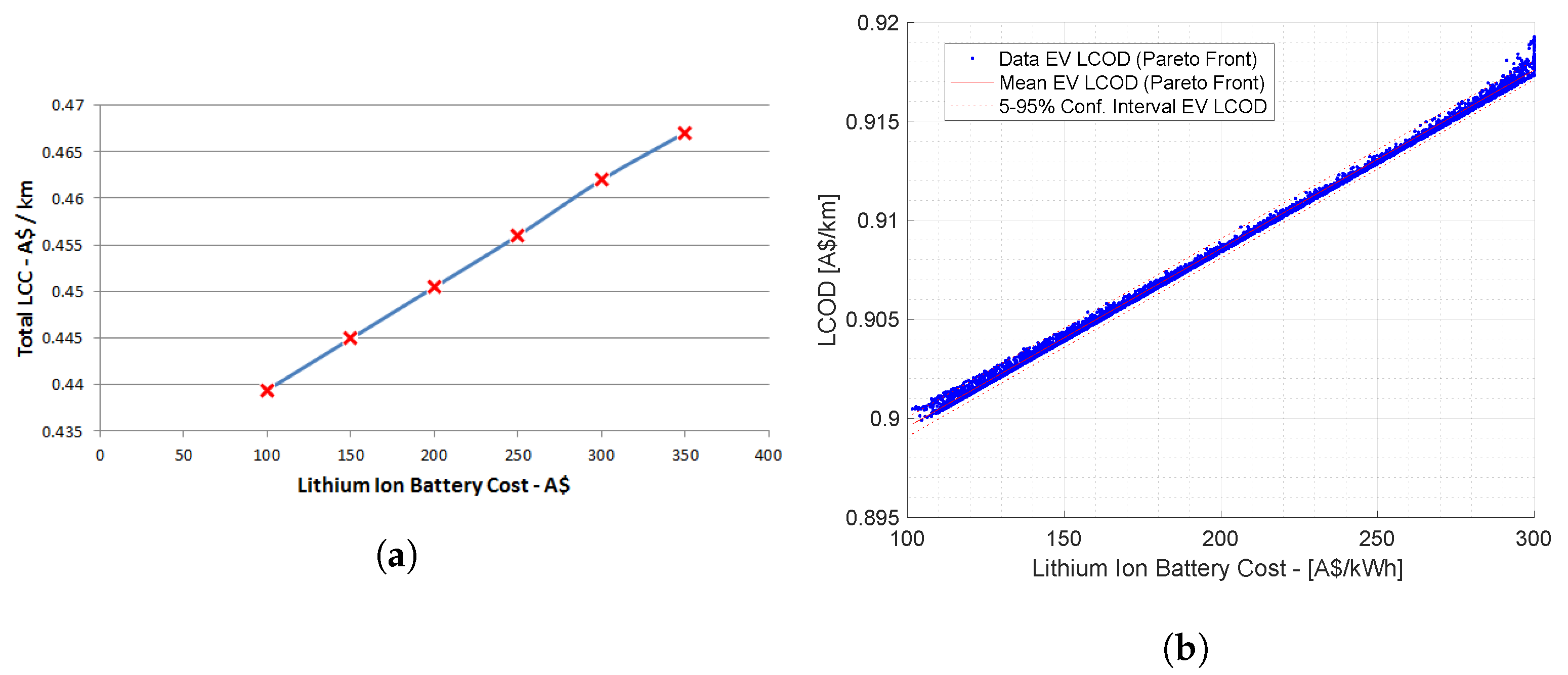
4.7. Comparison with Another Methodology

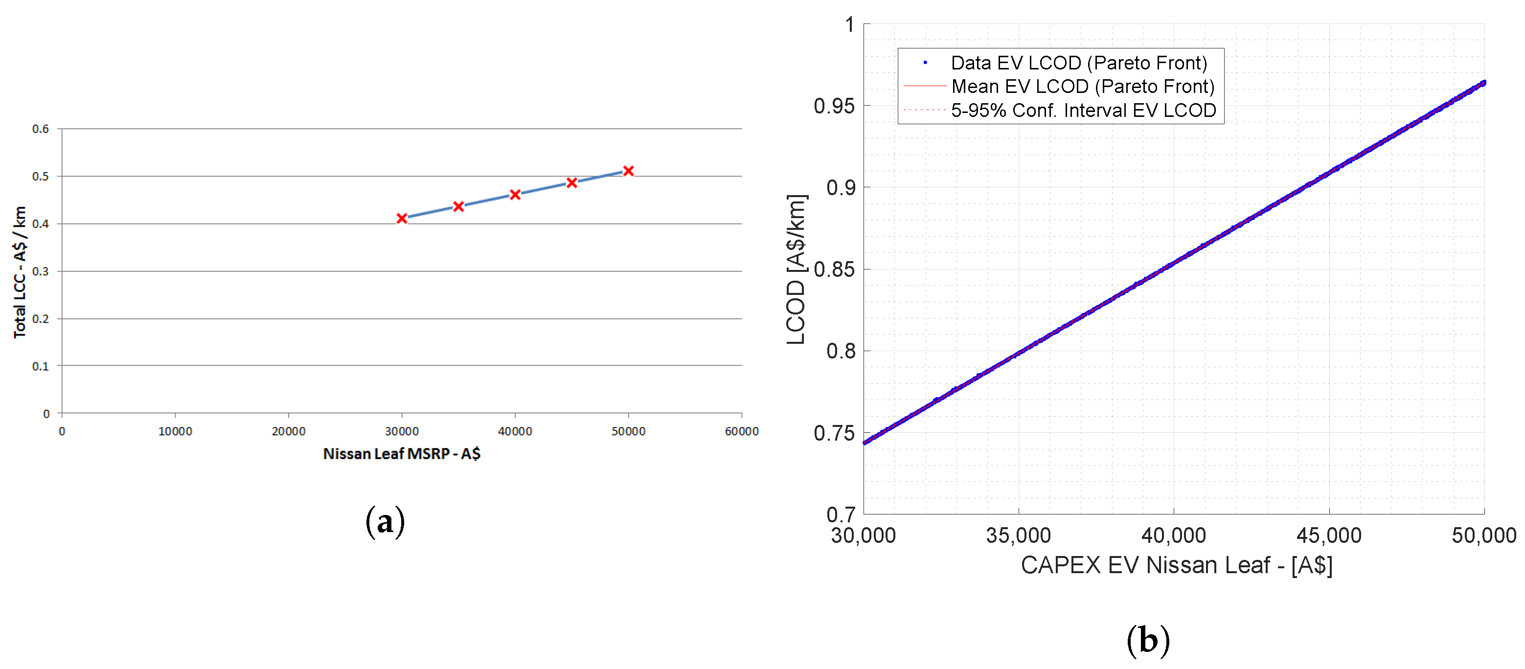
A comparison is made with the method and case study applied in Australia in [12], which has the data from

Table 5. Case study parameters of [12].

Parameters	EV
Economic Parameters
EV	2011 Nissan Leaf
CAPEX [A$]	$39,990
	+ Level 2 standalone charger: $3000
	+ Insurance and stamp duty taxes: $2352.7
Residual Value (RV)	$-
Battery price (B) [A$]	$5725
Maintenance Fee (K) [A$/km]	$0.038 + $0.024 (for tires)
Disposal Costs (DC) [A$]	$1935
Insurance Cost [A$/year]	$2452
Lifespan	200,000 km (20 years)
Technical features
Battery capacity [kWh]	24
EV range [km]	175
EV performance in the City [km/kWh]	6.66
EV charging inefficiency	20%
Energy consumption fee
Electric fee [A$/kWh]	off-peak hours: $0.16522, on-peak hours: $0.35046
	80% off-peak charging and 20% peak charging
NPV parameters
Discount rate	7%

for analysis. Data and results are in Australian dollars.

The annual route of the EV considered in the case study of [12] is 10,000 km per year, that is, 200,000 km in the useful life of the EV (without considering a stochastic behavior in the route), which corresponds to a journey by use of the EV in a conventional family, and not high journeys such as that of a taxi; 100 EV simulations are performed, which are shown in the Figure 7b, Figure 8b and Figure 9b.

The LCOD values with the proposed methodology are higher than the LCOD obtained based on the LCC in [12]. The difference in the results is due to the fact that [12] does not consider the following in its model: it does not include battery degradation in its model, which corresponds to a 10% increase in the method proposed by consider battery degradation. The discount rate does not apply to the annual flows of the route, which corresponds to a difference between 200,000 km (without discount) and 105,940 km (with discount) throughout the evaluation period (20 years), and this represents an affectation of the 80% increase in LCOD results. This difference will be less while the project is evaluated for less time or vice-versa.

4.8. Discussion

The economic principle of the Levelized Cost is based on what is evaluated with $NPV=0$, $r=IRR$, to obtain the formulation in (2), in which, in the denominator, the annual run contemplates the discount rate for the flow of each year.

In [7] the authors do not apply the discount rate to the annual run in the formulation of the LCOD, which could lead to inaccuracies in the results.

In [10,12] they obtain the LCOD from the relationship between the LCC and the annual trip (km), without applying the discount rate to the annual trip. This corresponds to an incorrect application of the LCOD concept, which leads to inaccuracies in the results.

Therefore, the LCOD and the LCC are not comparable to each other because their formulation, objectives, economic principles, and units are different.

Regarding the results obtained with the proposed methodology, the main barrier identified for electric mobility to be competitive and even with better prices per KM than the ICV, is the high CAPEX of the EV. The operating costs of the EV are lower than the ICV but the high CAPEX of the EV considerably affects the performance of the LCOD. However, the EV-LCOD is better performing than the ICV (refueling cost 4.66 USD/GL).

On the other hand, the performance of the EV-LCOD is subject to important variables that intervene in its model, which are considered in this article: CAPEX, residual value, discount rate, EV Charging Electric Rate, Vehicle performance and Battery Degradation. Although the proposed methodology does not implicitly analyze other factors that other authors contemplate in Table 1, such as: government incentive, taxes, social externalities, insurance, and disposal costs, these incentives and costs directly influence the CAPEX, for which the sensitivity of the CAPEX proposed in this article could be used.

The case studies analyzed in this article have not been applied to Hybrid Electric Vehicles (HEVs), for which it is necessary to consider the particularities of hybrid mobility technology.

5. Conclusions

This research work presents a bibliographic review on the application of the concept of Levelized Cost of Driving (LCOD) in electromobility, demonstrating that dissimilar criteria have been used by authors in its application. Moreover, inspired by the latter, we hereby propose a novel and holistic redefinition of the concept of the LCOD. The calculation of the proposed LCOD includes the most relevant expenses in the financial analysis, among them: a Monte-Carlo-based model to characterize the stochasticity associated with daily journeys of the vehicle, a battery state-of-health degradation model that incorporates information from different operating conditions, CAPEX, OPEX, discount rate, EV Charging Electric Rate, Vehicle performance, second life, and battery re-purposing (residual value). The proposed methodology is applied to contrast the performance of electric vehicles and ICV when they are used as taxis in the South American city of Quito, Ecuador. The relevance of having a good battery degradation model is clearly quantified, due to its implication on the financial analysis. A sensitivity analysis on the most important variables that affect the LCOD was performed using the concept of the Pareto front, helping to identify which conditions make an EV competitive with respect to the ICV. It should also be noted that these financial analyses are naturally based on actual prices, operating conditions, technological advances in vehicles, and the current economic situation of each country; therefore, it is always recommended to apply the proposed financial analysis with up-to-date and local data before reaching a definitive conclusion in other contexts.

The article analyzes the comparison of the LCOD with respect to the unit value of $/km that is calculated based on the LCC, which allows for identifying why there is a difference between both methodologies. The correct application of the Levelized Cost methodology is important to avoid errors with relevant magnitudes that could lead to misquantifying the unit costs that traveling with EV and ICV represent. Similarly, in the case where the LCC is used to determine the Levelized Cost, it must be done considering the economic principle with which the Levelized Cost was conceived (NPV = 0, and r = IRR).